Value of Cargo Pooling in On-Demand Intra-City Freight Logistics

Abstract

On-demand intra-city freight logistics (ICFL) has recently emerged as a new freight service, where shippers can submit their shipping requests using smartphones and be matched to drivers in real time based on their locations and drivers’ availability. A major challenge faced by on-demand ICFL platforms is the shortage of vehicles during peak demand periods. Cargo pooling, the cargo version of carpooling, offers as a promising way to increase supply: cargoes heading in the same direction would share the cargo compartment of the same vehicle and be serviced simultaneously, which is achieved by careful sequencing of the pickup and delivery locations of the cargoes. We investigate models for cargo pooling for on-demand ICFL and quantify its benefit, which is new to the literature. The major difference between existing studies on ICFL and ours is that we no longer assume that demands are known beforehand. Instead, the demands arrive gradually throughout the day and we need to periodically match requests to drivers and re-optimize vehicle routes. We formulate the matching problem as a dynamic pickup and delivery problem with three-dimensional loading and time window constraints. To solve this model, we develop an algorithm based on large neighborhood search and tree search. The algorithm is tested with real freight data in a city in the Yangtze River Delta. Results show that the algorithm can reduce the total cost by 21.4% and reduce the total vehicle miles traveled by 36.0%.

Keywords

on-demand intra-city freight logistics cargo pooling 3D-Loading time window pickup and delivery problem

The widespread use of smartphones has created a variety of on-demand services, for example, on-demand food delivery and on-demand ride hailing. Recently, intra-city freight logistics (ICFL) has also become on-demand, where a shipper can submit their shipping request—the pickup and delivery locations, the earliest pickup time (EPT) and the latest delivery time (LDT), and the type and dimension of the cargo—using smartphones and being matched to drivers in real time based on their locations and drivers’ availability. It is reported that the ICFL market in mainland China increased from 893.1 billion CNY (132.4 billion USD) in 2017 to 1,319.9 billion CNY (195.7 billion USD) in 2021, with an average annual compound growth rate of more than 10% ( 1 ). Furthermore, from 2017 to 2021, the market penetration rate of on-demand ICFL increased from 0.6% to 2.9%, and is expected to reach 19.8% by 2025 ( 1 ).

On-demand ICFL differs from other kinds of freight services in several ways. (i) It is on-demand because the shipping requests are received throughout the day and need to be matched to drivers in real time. Requests stay valid unless they cannot be matched with drivers within a time limit. (ii) It is intra-city because the pickup and delivery locations are within the urban area of a city. (iii) The cargo typically weighs between 30 kg and 500 kg and can be anything from furniture and luggage bags to hardwood floors and grocery/fruit pallets. (iv) The cargo needs to be picked up and delivered during the day, typically between 8:00 a.m. and 8:00 p.m. (v) The cargo is transported using cargo vans or small pickup trucks, as shown in Figure 1. This is because many Chinese cities prohibit medium-sized to large trucks from entering urban areas as a way to alleviate congestion during the day, which makes cargo vans and small trucks the only choices for ICFL. For ease of discussion, we use the term vehicles to refer to both cargo vans and small trucks used in ICFL. (vi) The cargo in a single shipment often does not take up the entire cargo compartment of a vehicle. The six characteristics of on-demand ICFL make it a crucial component of urban logistics. In comparison with other freight services, on-demand ICFL excels in meeting the personalized, on-demand freight needs of customers.

Figure 1.

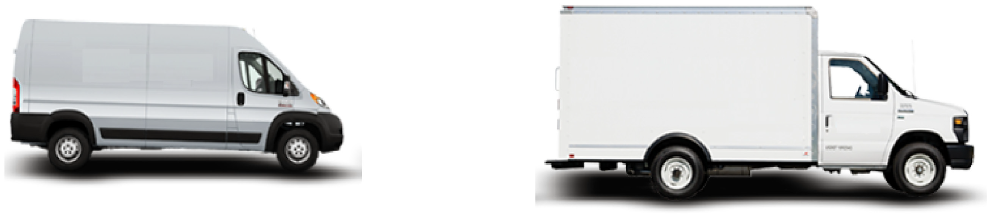
Intra-city freight logistics (ICFL) relies on cargo vans and small trucks to transport cargoes.

A major challenge faced by on-demand ICFL platforms is the shortage of vehicles during peak demand periods. At present, on-demand ICFL platforms provide dedicated services to shippers. A vehicle is dispatched to fulfill shipping requests one at a time and the vehicle will not pick up a new shipment until the shipment onboard has been delivered. This means that the cargoes are transported in a point-to-point way without intermediate stops and no two requests co-exist in the cargo compartment of a vehicle. Consider the example shown in Figure 2a. At 12:45 p.m. there are two shipping requests, where the pickup and delivery locations of the first one are indicated as P1 and D1, respectively. Its EPT and LDT are 1:00 p.m. and 1:30 p.m., respectively. The pickup and delivery locations of the second one are P2 and D2, respectively. Its EPT and LDT are 1:10 p.m. and 1:40 p.m., respectively. The travel times between P1 and P2, between P2 and D1, and between D1 and D2 are all 15 min. Assume that there is only one vehicle available and it is located at O, the platform can only take one of the two shipping requests while rejecting the other one.

Figure 2.

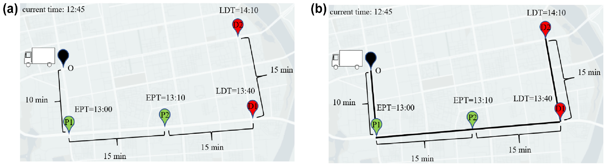
Cargo pooling can effectively increase supply and serve more requests: (a) when the platform provides dedicated services to shippers, only one shipping request can be served and (b) when the platform offers cargo pooling, both shipping requests can be served.

Cargo pooling, the cargo version of carpooling, has recently emerged as a way to increase supply during peak demand periods: cargoes heading in the same direction share the same cargo compartment and are serviced simultaneously, which is achieved by careful sequencing of the pickup and delivery locations of multiple cargoes. This offers a great opportunity to better utilize the capacities of the vehicles and serve more shippers. Let us continue with the example shown in Figure 2a. When cargo pooling is allowed, the platform can use the single vehicle available to accommodate both shipping requests following the black pickup/delivery route shown in Figure 2b. Under cargo pooling, since the vehicles need to make intermediate stops to pick up and deliver cargoes, the transportation time of a single request may increase. However, the utilization of the cargo compartments of the vehicles is improved and the total distance traveled is also reduced. As the transportation time for a single request may be prolonged with cargo pooling, the logistics company offers a lower price for this service as compensation. This allows shippers to take advantage of cost savings for the transportation of their cargo.

Though cargo pooling is a quite new service, similar ideas have appeared in other experiences of pooling in freight logistics in different regions of the world. Montoya-Torres et al. ( 2 ) studied a situation where three companies distributed goods to their stores. They compared the situation of the three companies delivering their goods separately and one company delivering all the goods in the form of cargo pooling. They used real data from the city of Bogotá, Colombia, for simulation. Pan et al. ( 3 ) introduced goods pooling strategies in supply chain transportation. Their model was tested with real data for 12 weeks of two French retailers and significantly reduced the CO₂ emissions. Kay et al. ( 4 ) demonstrated the economic impact of consolidation on transportation costs. The real data sets they used were produced using real city and town coordinates and population densities of Turkey. Therefore, there has been research on cargo pooling all over the world since 2010, but the situations mentioned above are all different from on-demand ICFL.

In this research, we quantify the value of cargo pooling in on-demand ICFL. The studies that are most closely related to our work are those on cargo pooling under static ICFL, where all shipping requests are received before any vehicle is dispatched. This problem is usually modeled as a pickup and delivery problem (PDP) with side constraints, which include: (i) capacity constraints, which measure whether a group of cargoes can fit into the cargo compartment of a vehicle. When only the weights of the cargoes are considered in the capacity constraints, they are called the cardinality constraints; when the dimensions of the cargoes are considered in the capacity constraints, they become the three-dimensional loading (3D-Loading) constraints; and (ii) time window constraints, which specify the time intervals when a cargo can be picked up from the origin and when it can be delivered to the destination. Table 1 compares our research with existing studies and illustrates the differences. Männel and Bortfeldt ( 5 , 6 ) investigated the PDP with 3D-Loading constraints. They assumed that the cargoes should strictly meet the first-in-last-out rule. Wu et al. ( 7 ) improved a hybrid heuristic algorithm for solving PDPs with 3D-Loading constraints without time window constraints. Dupas et al. ( 8 ) developed a mathematical model using combinatorial configurations approach for the PDP with 3D-Loading constraints. Stamadianos et al. ( 9 ) proposed a decision support system for the PDP with 3D-Loading constraints, considering multiple criteria. Our work is also remotely related to studies on the vehicle routing problem (VRP) with side constraints, where goods are transported between depots and customers. Gendreau et al. ( 10 ) was the first to look at the VRP with 3D-Loading constraints. Bortfeldt and Homberger ( 11 ) and Reil et al. ( 12 ) studied the VRP with 3D-Loading and time window constraints and developed a two-stage heuristic. Moura ( 13 ) presented a mixed integer linear programming model that characterized the 3D-Loading VRP with time windows.

Table 1.

Comparison Between Existing Studies and Our Research

Reference	Problem type	Capacity constraints	Time window constraints	On-demand
Li and Lim ( 14 )	PDP	Cardinality	✓	X
Ahkamiraad and Wang ( 15 )	PDP	Cardinality	✓	X
Wang et al. ( 16 )	PDP	Cardinality	✓	X
Sitek et al. ( 17 )	PDP	Cardinality	✓	X
Männel and Bortfeldt ( 5 )	PDP	3D-Loading	X	X
Männel and Bortfeldt ( 6 )	PDP	3D-Loading	X	X
Wu et al. ( 7 )	PDP	3D-Loading	X	X
Dupas et al. ( 8 )	PDP	3D-Loading	X	X
Stamadianos et al. ( 9 )	PDP	3D-Loading	X	X
Gendreau et al. ( 10 )	VRP	3D-Loading	X	X
Bortfeldt and Homberger ( 11 )	VRP	3D-Loading	✓	X
Reil et al. ( 12 )	VRP	3D-Loading	✓	X
Moura ( 13 )	VRP	3D-Loading	✓	X
This paper	PDP	3D-Loading	✓	✓

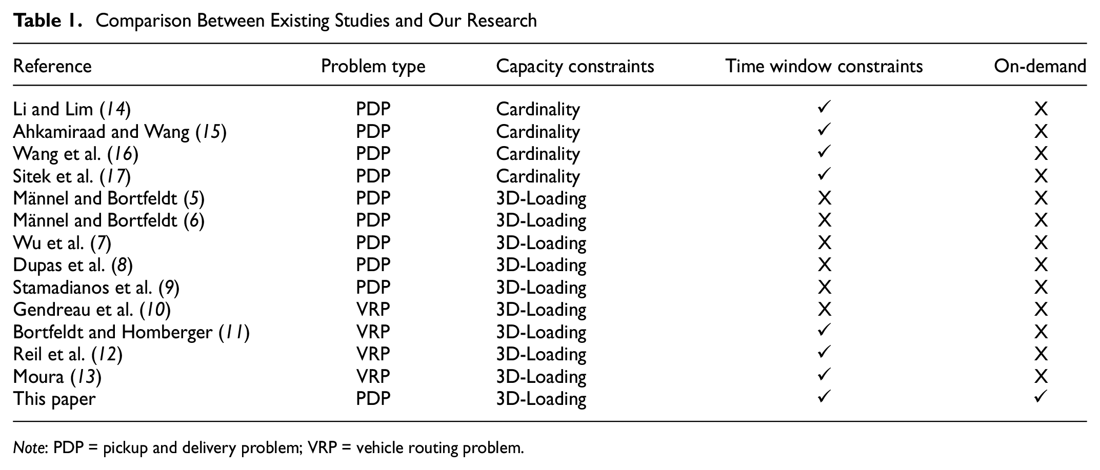
Note: PDP = pickup and delivery problem; VRP = vehicle routing problem.

We are the first to investigate cargo pooling in on-demand ICFL, which is new to the literature. The major difference between existing studies on ICFL and ours is that we no longer assume that demands are known beforehand, which is referred to as the static ICFL. Instead, the demands arrive gradually throughout the day and we need to periodically match requests to drivers and update vehicle routes. In each match, we take as input the demands received since the previous match as well as those that were received before the previous match but are still valid, the availability of the vehicles (their respective locations and the remaining capacities of the cargo compartments), and the pickup/delivery routes assigned to vehicles in the previous match. We then output vehicle routes and the storage plans of the cargoes inside the cargo compartments of the vehicles. We formulate the problem as a dynamic PDP with 3D-Loading and time window constraints. Existing researches tend to adopt heuristic algorithms to solve the PDP with 3D-Loading constraints ( 5 , 6 , 8 , 10 , 16 , 18 , 19 ). Since our problem is more complex because of the time windows, dynamic property, and larger scale of data, we adopt a hybrid heuristic algorithm. For PDPTW, which is a special case of dynamic PDP with 3D-Loading and time window constraints, Ropke and Pisinger ( 20 ) and Bent and Van Hentenryck ( 21 ) achieved outstanding results especially for larger instances through neighborhood search methods, while the method of tabu search was proved to be very successful for smaller instances by Li and Lim ( 22 ). Our hybrid heuristic algorithm is composed of a modified large neighborhood search algorithm by Männel and Bortfeldt ( 5 ) and Ropke and Pisinger ( 20 ) and a tree search algorithm by Chen et al. ( 23 ). The algorithm is tested with real freight data in a city in the Yangtze River Delta, China. Results show that cargo pooling can reduce the overall cost by 21.4% and reduce the total vehicle miles traveled by 36.0%. We summarize the contributions of our research as follows:

We are the first to investigate cargo pooling in on-demand ICFL, where demands are gradually received during the day.

We model the problem as a dynamic PDP with 3D-Loading and time window constraints, and develop a solution approach that periodically optimizes the pickup and delivery routes of vehicles.

The algorithm is tested with real freight data in a city in the Yangtze River Delta.

The remainder of this paper is organized as follows. In the next section, we introduce our notation and terminology. In the “Problem Definition” section, we present the definition for the cargo pooling problem. In the “Solution Approach” section, we develop a solution algorithm based on large neighborhood search and tree search. The “Numerical Experiments” section presents the dataset description, experimental setup, main results, analysis of the main results, and sensitivity analysis. The final section concludes the discussion and outline possible future research directions.

Notation and Terminology

In on-demand ICFL, customers submit shipping requests to the platform “24/7” and expect to be matched to a driver in real time. When a shipping request is received, its status is set to open. Once it is matched to a driver, its status becomes matched. If a shipping request cannot be matched to a driver in a given amount of time, for example, 30 min, it is rejected. On the side of the platform, it periodically, for example, every 10 min, invokes a matching procedure. Each time before the matching procedure is called, the platform gathers the following inputs: (i) the shipping requests that are open, which include those received since the previous matching and those that were received before the previous matching but have not been matched; (ii) the availability of the vehicles, including their locations and the remaining capacities of the cargo compartments; and (iii) the existing pickup and delivery routes assigned to the vehicles. The matching procedure then re-optimizes the pickup and delivery routes assigned to the vehicles as well as the way cargoes are stored in the cargo compartments of the vehicles.

The goal of this research is to develop a matching, or a re-optimization, model to facilitate cargo pooling. Now, let us define our notations. Suppose that there are $u$ open requests denoted as $R = {r_{1}, r_{2}, . . ., r_{u}}$ , and let $M$ be the set of matched requests. For a request, we know its pickup and delivery locations, EPT and LDT, weight, and dimensions (length × width × height). We number the pickup and delivery locations of open requests so that request $r_{i}, \forall i \in {1, 2, \dots, u}$ needs to be picked up from location $i$ and delivered to location $u + i$ . This implies that $P = {1, 2, . . ., u}$ is the set of pickup locations and $D = {u + 1, u + 2, . . ., 2 u}$ is the set of delivery locations. For request $i$ , let $θ_{i}$ be its EPT at location $i$ and $θ_{u + i}$ be its LDT at location $u + i$ .

Let us suppose that there are $μ$ vehicles denoted as $V = {v_{1}, v_{2}, . . ., v_{μ}}$ . Among these $μ$ vehicles, there are two types, where $μ_{1}$ vehicles are small trucks and $μ_{2}$ vehicles are cargo vans. These two types differ in the sizes of the cargo compartments. For vehicle $v_{i} \in V$ , we know its type, speed, cost per mile, size of cargo compartment, and maximum cruising range. Besides, let $M_{i}$ be the set of cargoes already in vehicle $v_{i}$ ’s cargo compartment. We know how they are stored and their delivery locations, $D_{i}^{'}$ .

Each time we re-optimize, we need to determine the vehicle’s route plan which can be described with the following parameters. $n_{k}, \forall k \in {1, 2, \dots, μ}$ denotes the number of locations that vehicle $v_{k}$ should go to; $a_{i, k} \in P \cup D \cup D_{k}^{'}, \forall i \in {1, 2, \dots, n_{k}}, \forall k \in {1, 2, \dots, μ}$ denote the ith location that vehicle $v_{k}$ should go to. If $a_{i, k} \in P$ , then vehicle comes to the pickup location of request $r_{a_{i, k}}$ to pick up cargoes; if $a_{i, k} \in D$ , then the vehicle comes to the delivery location of request $r_{a_{i, k} - u}$ to deliver cargoes. The route of vehicle $v_{k}$ can then be expressed as $[a_{0, k}, a_{1, k}, a_{2, k}, . . ., a_{n_{k}, k}]$ , where $a_{0, k}$ denotes the original location of vehicle $v_{k}$ . Since the vehicles are not empty from the start, the route of vehicle $v_{k}$ should contain the delivery locations of cargoes in $M_{k}$ and other location origin–destination (OD) pairs of new requests. That is, $D_{k}^{'} \subseteq {a_{0, k}, a_{1, k}, a_{2, k}, . . ., a_{n_{k}, k}}$ .

In the re-optimization, to minimize the total cost, we need to optimize the route of vehicle $[a_{0, k}, a_{1, k}, a_{2, k}, . . ., a_{n_{k}, k}], \forall k \in {1, 2, \dots, μ}$ . It is worth mentioning that the route of vehicle $v_{k}$ must contain the delivery locations of cargoes in $M_{k}$ . Therefore, more precisely for vehicle $v_{k}, \forall k \in {1, 2, \dots, μ}$ , we first need to match open requests to it, then obtain careful sequencing of location OD pairs of newly matched requests and those delivery locations of cargoes in $M_{k}$ .

Problem Definition

In each re-optimization, the problem can be modeled as a PDP with 3D-Loading and time windows constraints (3L-PDPTW) which has an initial solution with unbreakable structure. To introduce these problems better, we divide the discussion into two parts. The first part introduces the 3D-Loading Problem and the second part introduces the 3L-PDPTW.

3D-Loading Problem

Checking whether a vehicle is able to load the cargoes when it arrives at a pickup point is a 3D-Loading problem. Let $v$ denote the number of cargoes needed to be loaded. We need to determine whether $v$ 3D rectangular cargoes $G = {g_{1}, g_{2}, . . ., g_{v}}$ with length, width, height as $(l_{i}, w_{i}, h_{i}), \forall i \in {1, 2, \dots, v}$ can be placed into a bigger 3D rectangular cargo compartment with length, width, height as $(L, W, H)$ . We define the following parameters to determine the rotation of each cargo and the relative position of cargoes:

Define the vertical direction as the Z axis, the short-side direction of the compartment as the X axis, and the long-side direction as the Y axis. Cargoes can only rotate around the Z axis, so they can only have two orientations. Parameters $R_{i}$ are binary variables, representing the orientation of each cargo. If $R_{i} = 1$ , the length of cargo is parallel to the length of cargo compartment. Otherwise $R_{i} = 0$ , the width of cargo is parallel to the length of cargo compartment.

To determine the relative position between cargo $g_{i}$ and $g_{j}$ , we define three matrices ${(\begin{matrix} x_{ij} \end{matrix})}_{v \times v}$ , ${(\begin{matrix} y_{ij} \end{matrix})}_{v \times v}$ , and ${(\begin{matrix} z_{ij} \end{matrix})}_{v \times v}$ , where $x_{ij}, y_{ij}, z_{ij}$ are binary variables. If $i = j$ , $x_{ij} = y_{ij} = z_{ij} = 0$ . If cargo $g_{i}$ is to the left of cargo $g_{j}$ and cargo $g_{i}$ will overlap cargo $g_{j}$ when moving right, $x_{ij} = 1$ ; otherwise $x_{ij} = 0$ . Similarly, if cargo $g_{i}$ is in front of cargo $g_{j}$ and cargo $g_{i}$ will overlap cargo $g_{j}$ when moving behind, $y_{ij} = 1$ ; otherwise $y_{ij} = 0$ . If cargo $g_{i}$ is on the top cargo $g_{j}$ , $z_{ij} = 1$ and cargo $g_{i}$ will overlap cargo $g_{j}$ when moving down; otherwise $z_{ij} = 0$ .

Then ${R_{1}, R_{2}, \dots, R_{v}}$ , ${(\begin{matrix} x_{ij} \end{matrix})}_{v \times v}$ , ${(\begin{matrix} y_{ij} \end{matrix})}_{v \times v}$ and ${(\begin{matrix} z_{ij} \end{matrix})}_{v \times v}$ represent a kind of placement of cargoes. To find an available placement of cargoes, we need to ensure the constraints listed as follows:

Orientation constraints: Cargoes can only rotate around the Z axis.

\begin{matrix} l_{i}^{'} = R_{i} l_{i} + (1 - R_{i}) w_{i}, \forall i \in {1, 2, \dots, v}; \\ w_{i}^{'} = R_{i} w_{i} + (1 - R_{i}) l_{i}, \forall i \in {1, 2, \dots, v} . \end{matrix}

Nonoverlapping constraints: Cargoes cannot overlap. If $x_{ij} = 1, x_{jk} = 1$ , then $x_{ik} = 1$ . Similarly, if $y_{ij} = 1, y_{jk} = 1$ , then $y_{ik} = 1$ . If $z_{ij} = 1, z_{jk} = 1$ , then $z_{ik} = 1$ . Also, it is not allowed for there to be two relative positional relationships between any two cargoes at the same time.

x_{ij} + x_{ji} + y_{ij} + y_{ji} + z_{ij} + z_{ji} \leq 1, \forall i \in {1, 2, \dots, v}, \forall j \in {1, 2, \dots, v} .

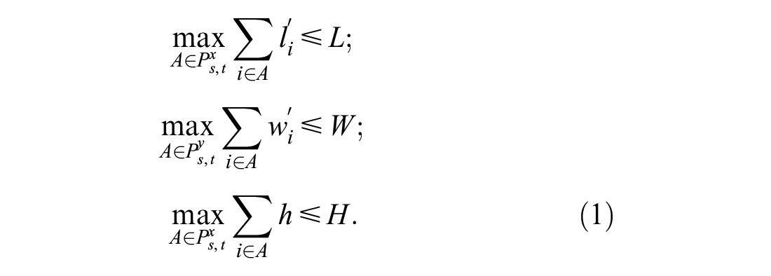
Supporting constraints: If a cargo is placed on the top of another, the upper surface of the lower cargo must fully support the lower surface of the upper cargo. That is, if $z_{ij} = 1$ , cargo $g_{i}$ are on the top cargo $g_{j}$ , then $l_{i}^{'} \leq l_{j}^{'}, w_{i}^{'} \leq w_{j}^{'}$ .

No exceeding constraints: The cargoes cannot exceed the compartment in the three directions of the X, Y, and Z axes. Take the X axis as an example. Let $S^{x} = {g_{s} | x_{is} = 0, \forall i \in {1, 2, \dots, v}}$ , then according to the definition of ${(\begin{matrix} x_{ij} \end{matrix})}_{v \times v}$ , there are no other cargoes to the left of cargo $g_{s} \in S^{x}$ . Similarly, let $T^{x} = {g_{t} | x_{ti} = 0, \forall i \in {1, 2, \dots, v}}$ , there are no other cargoes to the right of cargo $g_{t} \in T^{x}$ . Let $P_{s, t}^{x}$ denote all cargoes between $g_{s}$ and $g_{t}$ , including cargo $g_{s}$ and $g_{t}$ . That is, $P_{s, t}^{x} = {{p_{1}, p_{2}, \dots, p_{n_{0}}} | p_{1} \in S^{x}, p_{n_{0}} \in T^{x}, x_{p_{1} p_{2}} = x_{p_{2} p_{3}} = \dots = x_{p_{n_{0} - 1} p_{n_{0}}} = 1}$ . Then in the X axis, $max_{A \in P_{s, t}^{x}} \sum_{i \in A} l_{i}^{'} \leq L$ can ensure the cargoes cannot exceed the compartment in the direction of the X axis. Similarly define the $S^{y}, T_{y}, P_{s, t}^{y}, S^{z}, T^{z}, P_{s, t}^{z}$ , then the no exceeding constraints can be expressed as:

\begin{matrix} max_{A \in P_{s, t}^{x}} \sum_{i \in A} l_{i}^{'} \leq L; \\ max_{A \in P_{s, t}^{y}} \sum_{i \in A} w_{i}^{'} \leq W; \\ max_{A \in P_{s, t}^{x}} \sum_{i \in A} h \leq H . \end{matrix}

(1)

Loading order constraints: The cargoes placed earlier cannot be on top or in front of a cargo placed later.

\begin{matrix} y_{ij} = 0, \forall i \leq j; \\ z_{ij} = 0, \forall i \leq j . \end{matrix}

(2)

PDP with 3D-Loading and Time Windows Constraints

In every re-optimization, as shown in “Notation and Terminology,” we need to optimize the route of vehicle $[a_{0, k}, a_{1, k}, a_{2, k}, . . ., a_{n_{k}, k}], \forall k \in {1, 2, \dots, μ}$ to minimize the total cost of the logistics company. Then we introduce the cost function and constraints in detail. The cost consists of three parts: the cost of distance, the cost of reloading, and the penalty for late delivery. The total cost can be expressed as:

C_{total} = c_{dis} + c_{reload} + p_{delay} .

(3)

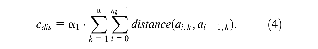
These three parts will be introduced in turn. We first introduce the cost of distance. We use Manhattan distance to approximate the actual distance between pickup and delivery locations, which is widely adopted in the literature ( 24 , 25 ). $distance (a_{i, k}, a_{i + 1, k})$ denotes the function of Manhattan distance between locations $a_{i, k}$ and $a_{i + 1, k}$ ; $α_{1}$ denotes the cost per mile, which is calculated as cargo van fuel consumption per mile multiplied by fuel price. Then the cost of distance can be expressed as

c_{dis} = α_{1} \cdot \sum_{k = 1}^{μ} \sum_{i = 0}^{n_{k} - 1} distance (a_{i, k}, a_{i + 1, k}) .

(4)

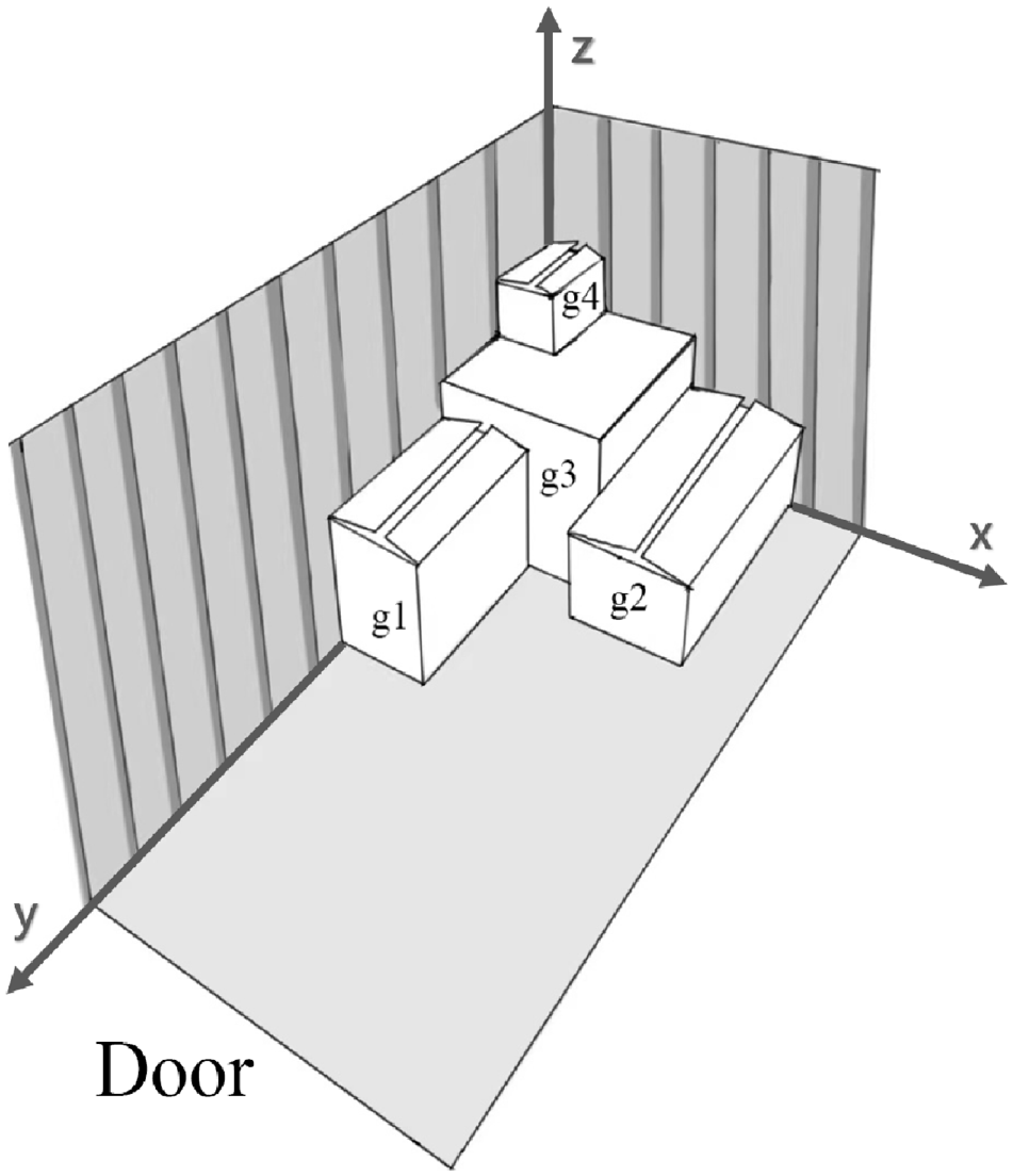
We then introduce the cost of reloading. As shown in Figure 3, there are four cargoes in the compartment. We assume that all cargo vans can only be opened on one side which is marked in the figure. There are no other cargoes that are closer to the door or are on top of cargo $g_{1}$ and $g_{2}$ . Therefore, cargo $g_{1}$ and $g_{2}$ are ready for unloading, which means we do not need to move other cargoes to unload cargo $g_{1}$ and $g_{2}$ . While cargo $g_{1}$ is closer to door than cargo $g_{3}$ and $g_{4}$ is on the top of $g_{3}$ , cargo $g_{3}$ is not ready for unloading, which means we should first unload cargo $g_{1}$ and $g_{4}$ to unload $g_{3}$ , leading to more unloading time and extra labor cost. Therefore, we take the cost of reloading into consideration.

Figure 3.

Illustration of possible placement of four cargo items in the cargo compartment.

We assume that any cargo put in the van later will definitely block the cargo put in the van earlier. This assumption is from the research of Männel and Bortfeldt ( 5 ). Essentially, considering reloading is a trade-off between the cost of distance and the cost of reloading. Ignoring reloading may give route planning more freedom, thereby reducing cost of distance. Conversely, making the route shorter may result in more reloading effort.

Let function $reload (k, i)$ denote whether vehicle $v_{k}$ needs to reload at location $a_{i, k}$ . If vehicle $v_{k}$ needs to reload at location $a_{i, k}$ , $reload (k, i) = 1$ , otherwise $reload (k, i) = 0$ ; constant $α_{2}$ denotes cost per time of reloading. Whether to reload at a delivery point is determined by judging whether there are unpaired locations between it and its pickup points. The cost of reloading can be expressed as

c_{reload} = α_{2} \cdot \sum_{k = 1}^{μ} \sum_{i = 0}^{n_{k}} reload (a_{i, k}) .

(5)

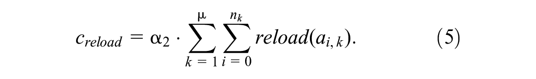
The last part of the cost function is the penalty for late delivery. In essence, cargo pooling is a way to reduce the total cost by properly extending a single request’s transportation time. For a shipper, cargo pooling may result in extended transit times, increasing the likelihood of missed delivery deadlines. It essentially penalizes the objective function if the delivery of a cargo cannot be made before its LDT. The goal is to produce a pickup/delivery schedule that tries to respect the LDTs of the cargoes, so we need to take the delay penalty into consideration. Constant $α_{3}$ denotes the penalty for late delivery for a delay of one minute. Function $delay (r_{i})$ denotes the time delayed for request $r_{i}$ . The penalty for late delivery can be expressed as

p_{delay} = α_{3} \cdot \sum_{r_{i} \in R \cup M} delay (r_{i}) .

(6)

After introducing the cost function, we introduce the constraints of our model. The constraints and rules of our problem are listed as follows:

No missing constraints: All requests should be delivered.

3D-Loading constraints: Each time a vehicle arrives at a pickup point, we should check whether cargoes can be loaded into the vehicle. This kind of checking can be modeled as a 3D-Loading problem, see section 3D-Loading Problem for details.

Weight constraints: Each time a vehicle arrives at a pickup point, we should check whether the sum of the cargoes’ weight will exceed the vehicle’s maximum weight capacity.

Maximum travel distance constraints: Each vehicle has a maximum travel distance. The total distance of a single trip of a vehicle should be less than the maximum travel distance.

Driving hour constraints: As is required by State Council of the PRC ( 26 ), after driving for 4 h, the driver of a vehicle must take a break of 20 min.

Maximum requests constraints: Each type of vehicle has a maximum number of requests that it can take at the same time.

Last-in first-out rules (LIFO): To avoid reloading, cargo that is later loaded into the vehicle should be unloaded first, as this avoids repeated movement of cargoes. If reloading is necessary, we add the cost of reloading to the cost.

Time windows rules: Each request should have an EPT and an LDT, and the vehicle should arrive at the designated location in these time windows. If a timeout is necessary, we add penalty for late delivery to the cost.

Solution Approach

To cope with on-demand requests, we need a dynamic algorithm to do cargo pooling repeatedly. And in each time period, we carry re-optimization with the information known. In this section we first introduce the framework of the algorithm, then introduce two algorithms used in cargo pooling: large neighborhood search (LNS) and tree search (TS).

Overall Solution Approach: Framework of Algorithm

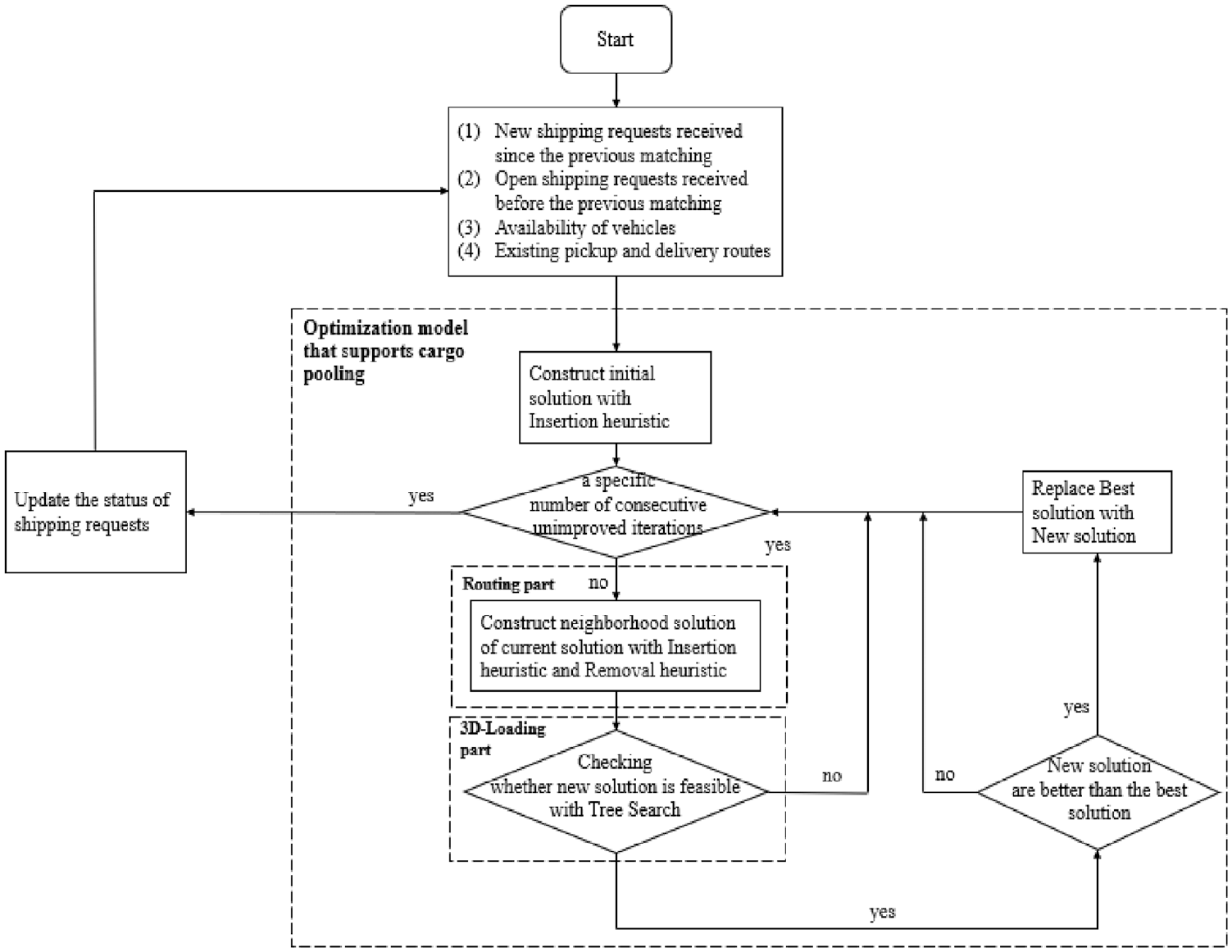
According to the model, the service hours of a day are divided into many 10 min intervals called time periods. In each time period, we perform re-optimization of cargo pooling. The process of the algorithm for cargo pooling is shown in Figure 4. In each re-optimization, we input: (i) the open shipping requests, (ii) the availability of vehicles, and (iii) the existing pickup and delivery routes. Then we perform re-optimization for cargo pooling with LNS and TS to obtain a new pickup and delivery route. The detailed optimization model is shown in the dotted box. After constructing the initial solution, if a specific number of consecutive unimproved iterations is not reached, the model will keep searching the neighborhood of the current solution. The routing part in the red dotted box is used to find a better solution, and the 3D-Loading part in the blue dotted box is used to ensure the feasibility of the solution. After re-optimization, we record the completed requests and update: (i) the open shipping requests, (ii) the availability of the vehicles, and (iii) the existing pickup and delivery routes. We then pass them to the next period. After finishing the last time period, we can use the data of all the completed requests to calculate the total cost and vehicle miles traveled to evaluate the benefits of on-demand cargo pooling.

Figure 4.

Solution framework for re-optimization.

We then introduce the detail of the state of vehicles and requests that will be rolling updated in each time period. Each request has four states: unassigned, assigned but not picked up, in transit, and delivered. If a request state is unassigned, it means this request has not been assigned to any vehicle and we can assign it to any vehicle that is available. If a request state is assigned but not picked up, it means that this request has been assigned to a vehicle but has not been started for pickup and we can still make adjustment to its pickup/delivery plan. If a request state is in transit, it means that this request has been assigned to a vehicle and this vehicle has already picked up the cargoes, then we must finish its delivery, but we still can adjust the delivery plan for other requests to change its transportation time. If a request state is delivered, it means that both the pickup and delivery of this request is done, we cannot do any removal or insertion to it. The state of vehicle $v_{k}$ contains the position of the vehicle at beginning of the time period $a_{0, k}$ and the set of cargoes already in cargo compartment $M_{k}$ . When doing removal, we cannot remove the delivery location of cargoes in $M_{k}$ .

LNS Algorithm

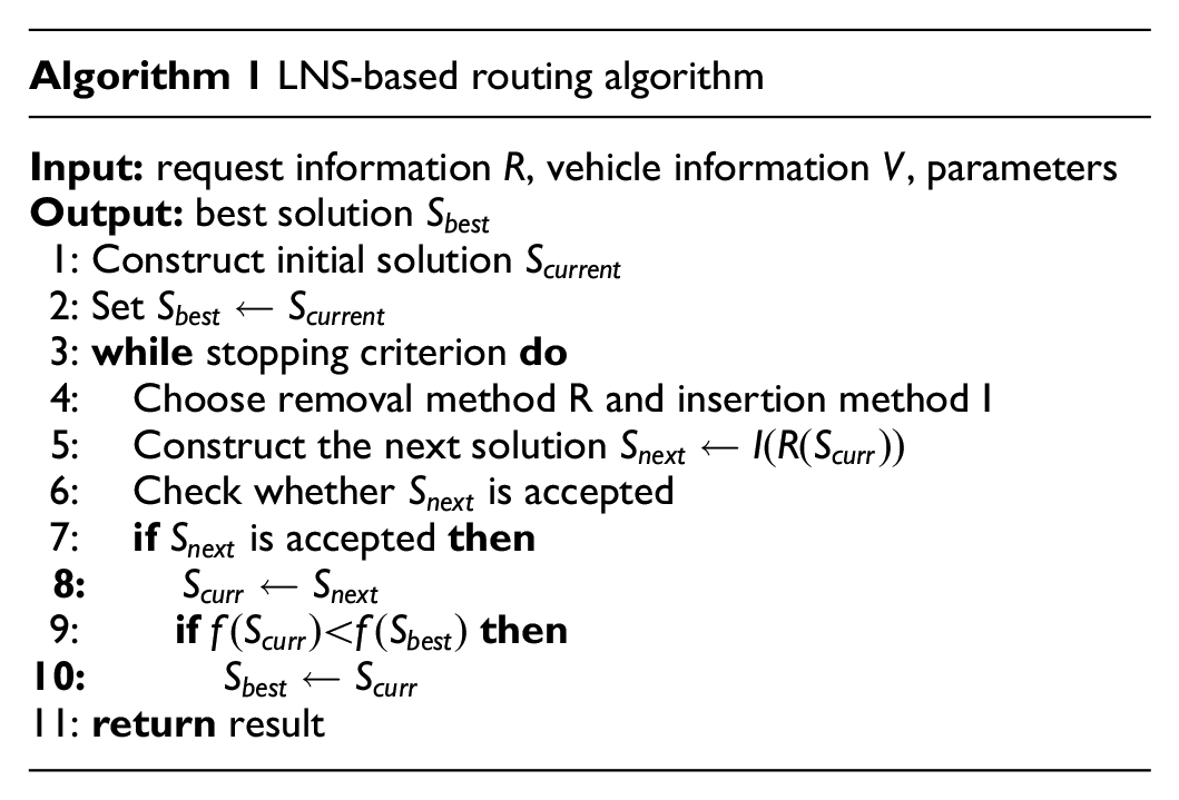
We adopt the LNS algorithm developed by Shaw ( 27 ) to solve the routing part of 3L-PDPTW. The LNS algorithm is a widely used heuristic algorithm that keeps finding better solutions by searching the “neighborhood” of the current solution. In LNS, the neighborhood is implicitly defined by destroy and repair methods. The destroy method destroys part of the current solution, and then the repair method rebuilds the destroyed solution. The destroy method usually contains an element of randomness to destroy a different part of the solution each time the destroy method is called. The main processes are shown in Algorithm 1. We construct the initial solution with greedy insertion in Line 1 and set it as the candidate for best solution in Line 2. Between Line 4 and Line 10 we carry the LNS. In each iteration, we randomly choose removal heuristic and insertion heuristic to find the neighborhood of $S_{current}$ in Lines 4 and 5. In Line 7, we check whether its neighborhood $S_{next}$ is accepted using a simulated annealing-based acceptance criterion. If so, we replace $S_{current}$ with $S_{next}$ in Line 8. And if $S_{next}$ has lower cost function, we replace $S_{best}$ with $S_{next}$ in Line 10. We repeat this process until the stopping criteria is satisfied, and we find the solution. Chen et al. ( 28 ) use a specific number of consecutive unimproved iterations as their stopping criteria, and we do the same.

Algorithm 1 LNS-based routing algorithm
Input: request information $R$ , vehicle information $V$ , parameters Output: best solution $S_{best}$ 01: Construct initial solution $S_{current}$ 02: Set $S_{best} \leftarrow S_{current}$ 03: while stopping criterion do 04: Choose removal method R and insertion method I 05: Construct the next solution $S_{next} \leftarrow I (R (S_{curr}))$ 06: Check whether $S_{next}$ is accepted 07: if $S_{next}$ is accepted then 08: $S_{curr} \leftarrow S_{next}$ 09: if $f (S_{curr}) < f (S_{best})$ then 10: $S_{best} \leftarrow S_{curr}$ 11: return result

Algorithm 1 LNS-based routing algorithm

Input: request information

R

, vehicle information

V

, parameters
Output: best solution

S_{best}

01: Construct initial solution

S_{current}

02: Set

S_{best} \leftarrow S_{current}

03: while stopping criterion do
04: Choose removal method R and insertion method I
05: Construct the next solution

S_{next} \leftarrow I (R (S_{curr}))

06: Check whether

S_{next}

is accepted
07: if

S_{next}

is accepted then
08:

S_{curr} \leftarrow S_{next}

09: if

f (S_{curr}) < f (S_{best})

then
10:

S_{best} \leftarrow S_{curr}

11: return result

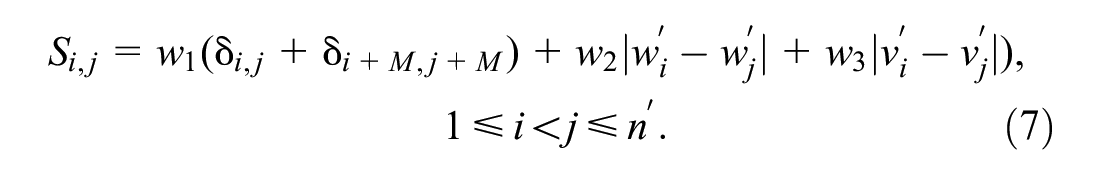
In our study, we destroy our current solution $S_{current}$ by removing requests, and we repair our solution by inserting removed requests to obtain a new feasible neighborhood solution $S_{next}$ . Detailed insertion rules and removal rules are introduced above in the “Overall Solution Approach: Framework of Algorithm” section. Let $I (S)$ denote the insertion heuristic and $R (S)$ denote the removal heuristic. The neighborhood searching process can then be expressed as $S_{next} = I (R (S_{current}))$ .

We use two kinds of insertion heuristic (greedy insertion, time insertion) and two kinds of removal heuristic (Shaw removal, random removal) in our model, which are introduced in this paragraph and the next two paragraphs. The Shaw removal, random removal, and greedy insertion methods are adopted from the adopted large neighborhood search heuristic devised by Ropke and Pisinger ( 20 ). Random removal randomly removes a request that has been assigned to a vehicle but has not been picked up. In on-demand cargo pooling, we track the state of each request and vehicle to mark whether they are available for removal and insertion. Therefore, we can only remove those requests that have been assigned to a vehicle but not been picked up. Greedy insertion traverses all the requests to be inserted, the vehicles to insert and the positions to insert, then selects one solution that causes the least cost increase. It is worth mentioning that this insertion is the most complex one, for it has to traverse all situations. Shaw removal removes the two assigned requests that are most similar between all assigned requests. The similarity between requests is calculated as follows:

S_{i, j} = w_{1} (δ_{i, j} + δ_{i + M, j + M}) + w_{2} | w_{i}^{'} - w_{j}^{'} | + w_{3} | v_{i}^{'} - v_{j}^{'} |), 1 \leq i < j \leq n^{'} .

(7)

The $distance (p_{i}, p_{j}), w_{i}^{'}, v_{i}^{'}$ lies in the interval $[0, 1]$ . $δ_{i, j}$ denotes the normalized distance between pickup position of request $r_{i}$ and $r_{j}$ ; $δ_{i + M, j + M}$ denotes the normalized distance between delivery position of request $r_{i}$ and $r_{j}$ ; $w_{i}^{'}$ denotes the normalized weight of request $r_{i}$ ; $v_{i}^{'}$ denotes the normalized volume of request $r_{i}$ ; $w_{1}, w_{2}, w_{3}$ denoted the weight of distance, weight and volume.

Besides these destroy and repair methods, we add time insertion, which inserts requests in chronological order. In this kind of insertion, we first sort all requests in order of LDT, traverse all the vehicles to insert and the position to insert, then select one solution that causes the least cost increase. Time insertion is similar to greedy insertion. Because of the lack of traversing of requests, time insertion can be done much faster than greedy insertion.

Tree Search

To solve the 3D-Loading problem, we adopt a TS algorithm developed by Chen et al. ( 23 ), which searches through a tree structure. Before introducing the algorithm, we first introduce the tree structure. Except for the root node, every node represents a kind of partial placement, the depth of node represents the number of cargoes this node has. For example, a node whose depth is four represents a kind of placement of ${g_{1}, g_{2}, g_{3}, g_{4}}$ . The link of two nodes means that the child node is generated from a parent node, and that the child node is to add a new cargo on the basis of the parent node. Each cargo has two orientations. Two cargoes have seven types of relative position, which are all one-hot code of $(x_{ij}, x_{ji}, y_{ij}, y_{ji}, z_{ij}, z_{ji})$ and (0,0,0,0,0,0). So if the placement of a parent node whose depth is $d$ is feasible, this node has at most $2 \times 7^{d}$ child nodes, for the new cargo itself has two orientations and each of the previous cargoes has seven kinds of relative position with new cargo. These $2 \times 7^{d}$ child nodes is not all feasible, we should check them with the constraints in section PDP with 3D-Loading and Time Windows Constraints. If one is feasible, we continue to construct its child node. And if the placement of a node is infeasible, this node does not have a child node. As shown in Figure 5, for example, 3-1 and 3-2 denote the orientation of $g_{3}$ , and (1,3) denote the seven relative position of cargo $g_{1}$ and $g_{3}$ . We use $I_{k}$ to represent the case with $k$ cargoes ${g_{1}, g_{2}, . ., g_{k}}$ . All nodes whose depth is $k$ form the case $I_{k}$ . Our search strategy is to use a depth-first approach to determine whether $I_{n}$ has a feasible node.

Figure 5.

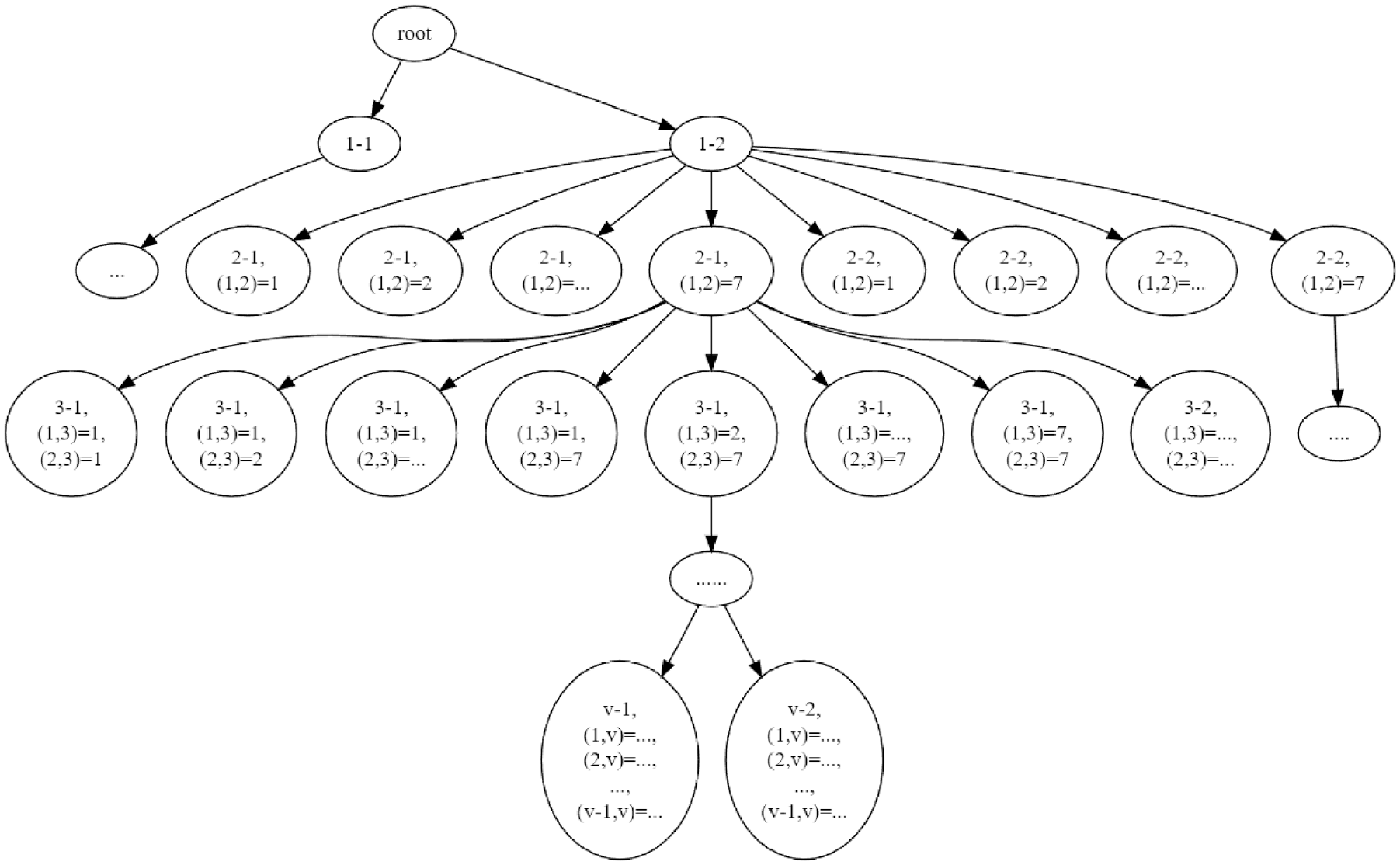
Illustration of the tree search algorithm.

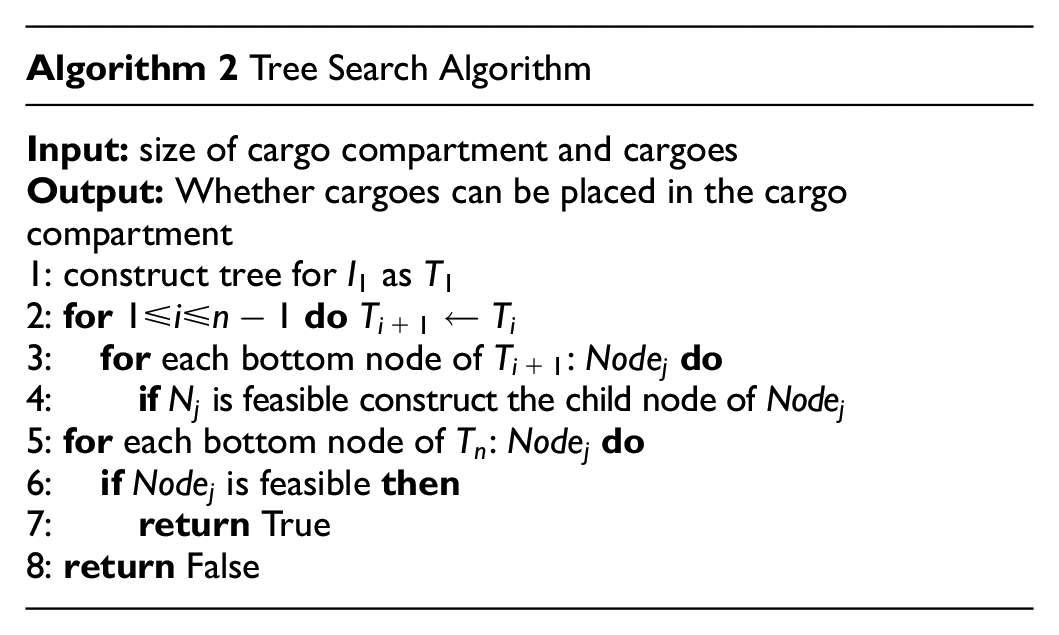
The process of the algorithm is shown in Algorithm 2. In Line 1, we construct the tree $T_{1}$ with $I_{1}$ . $T_{1}$ only has a root node and two child nodes which denote two orientations of cargo $g_{1}$ . Between Line 2 and 4, we construct the tree by adding cargoes. For example, we first to check whether the node of $I_{1}$ is feasible. Since $I_{1}$ contains one cargo $g_{1}$ , only two orientations need to be considered, which are 1-1 and 1-2. We construct the child for all feasible nodes in $I_{1}$ . Then we check whether the node of $I_{2}$ is feasible and construct the child for all feasible nodes in $I_{2}$ . In this way we construct a tree for $I_{n}$ . Then in Line 5 and 6, we check whether the bottom nodes of $I_{n}$ are feasible. If $I_{n}$ has no node whose depth is $n$ or all bottom nodes of $I_{n}$ are infeasible, there is no feasible solution for the 3D-Loading problem. Otherwise if there is a feasible node whose depth is $n$ , the placement it represents is a feasible solution for the 3D-Loading problem.

Algorithm 2 Tree Search Algorithm
Input: size of cargo compartment and cargoes Output: Whether cargoes can be placed in the cargo compartment 1: construct tree for $I_{1}$ as $T_{1}$ 2: for $1 \leq i \leq n - 1$ do $T_{i + 1} \leftarrow T_{i}$ 3: for each bottom node of $T_{i + 1}$ : $Nod e_{j}$ do 4: if $N_{j}$ is feasible construct the child node of $Nod e_{j}$ 5: for each bottom node of $T_{n}$ : $Nod e_{j}$ do 6: if $Nod e_{j}$ is feasible then 7: return True 8: return False

Algorithm 2 Tree Search Algorithm

Input: size of cargo compartment and cargoes
Output: Whether cargoes can be placed in the cargo compartment
1: construct tree for

I_{1}

T_{1}

2: for

1 \leq i \leq n - 1

T_{i + 1} \leftarrow T_{i}

3: for each bottom node of

T_{i + 1}

Nod e_{j}

do
4: if

N_{j}

is feasible construct the child node of

Nod e_{j}

5: for each bottom node of

T_{n}

Nod e_{j}

do
6: if

Nod e_{j}

is feasible then
7: return True
8: return False

Numerical Experiments

To quantify the value of cargo pooling for on-demand city logistics, we conduct numerical experiments on real datasets and perform a sensitivity analysis on some parameters. Computational experiments are organized in the following four parts: dataset description, experimental setup, main result, and sensitivity analysis. All procedures are coded in the Python programming language using Visual Studio Code. All experiments have been conducted on a personal computer with five CPU and 12 GB RAM.

Description of Dataset

We use real demand data for the numerical simulations. Input to our model includes the set of shipping requests (origins, destinations, EPTs, LDTs, cargo dimensions, and estimated shipping charges). The cargo compartment dimensions of two types of vehicles are as follows: (i) length 1.8, width 1.3, height 1.1 and (ii) length 2.7, width 1.4, height 1.2. The freight requests are extracted from data collected in December 2021 in a city in the Yangtz River Delta, including an average of 16,000 requests per day. We have selected 508,391 requests information that chose the cargo pooling option for the numerical experiment. To gain a more intuitive grasp of the data, we randomly selected 500 requests and drew lines connecting all the pickup locations and delivery locations, as shown in Figure 6. The yellow points denote the pickup location and the red points denote the delivery point. The straight-line distance between the pickup point and the delivery point for almost all requests is less than 25 km.

Figure 6.

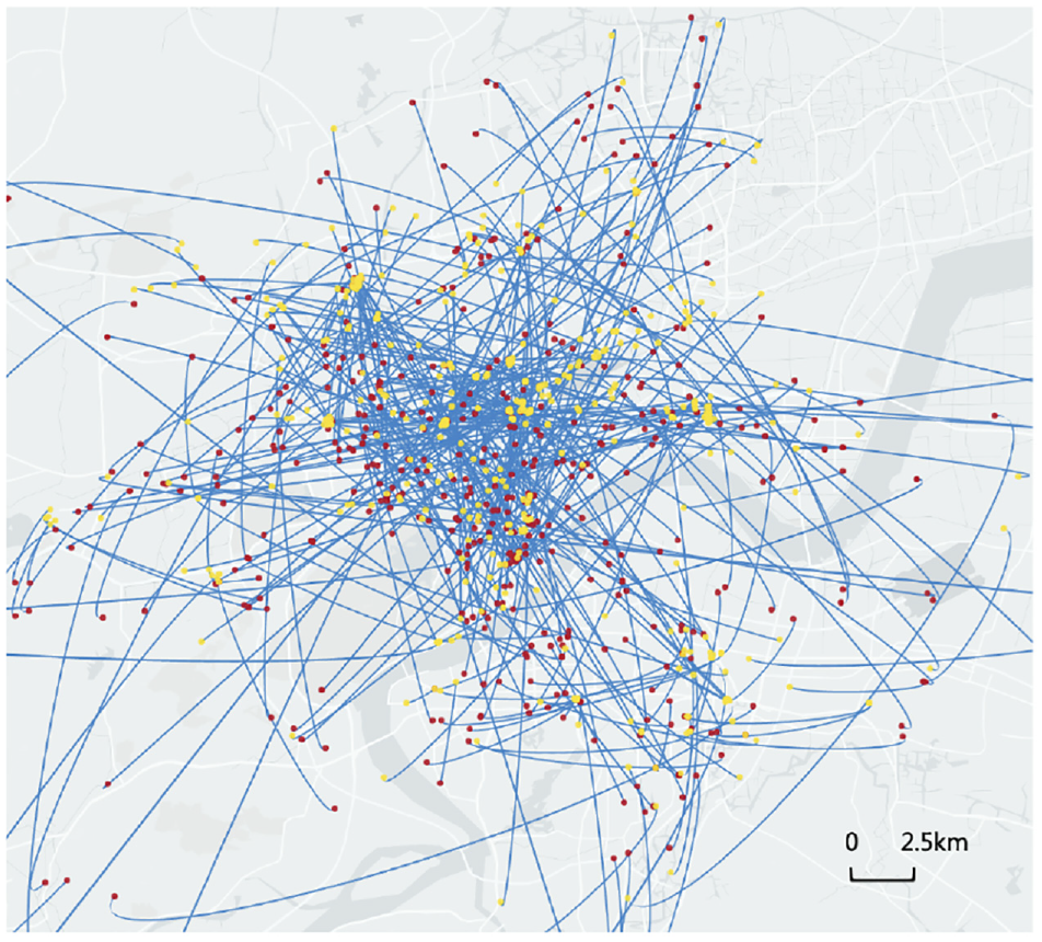
Geographical distribution of the sampling origin–destination pairs in our numerical tests.

To gain a better understanding of the datasets, we picked one of the days and plotted the results of number of requests received by time in percentage, as shown in Figure 7. Each data point on the line chart denotes the requests received in a 10 min interval, in percentage. We can tell that there are two peaks namely 10:00 in the morning and 14:00 to 15:00 in the afternoon. In addition, the histogram and cumulative distribution function of normalization results of transportation time in percentage are shown in Figure 8. We can tell that the vast majority of requests are delivered within an hour, a few requests take two hours to deliver, very few requests take more than two hours to deliver. Considering the business scenario, we mainly consider same-day and intra-city delivery. In data pre-processing, we eliminated requests that require more than a day for transportation and those with pickup and delivery points located in different cities. We then divided the remaining requests into time periods of 10 min each for input. It is worth mentioning that the LDT will be the actual delivery time. Since the actual time is too demanding for situation of cargo pooling, we will introduce the concept of time flexibility. In sensitivity analysis, we extend the LDT and repeat the experiment. The length of extended time is named the level of time flexibility.

Figure 7.

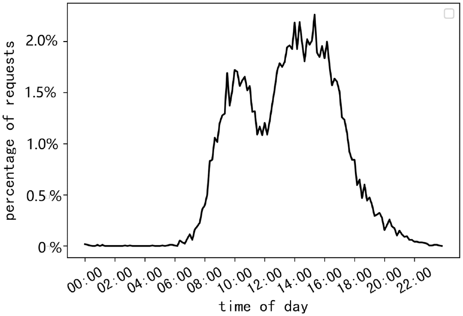
Distribution of the number of shipping requests received every 10 min.

Figure 8.

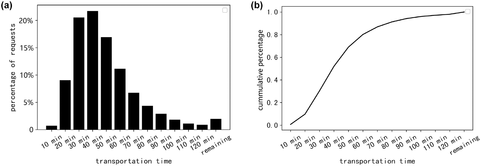
Descriptive statistics of transportation time: (a) distribution of the transportation times for completed shipping requests and (b) cumulative distribution of the transportation times for completed shipping requests.

Experimental Setup

In the experiment setup, we set the weights in Shaw removal as $(w_{1}, w_{2}, w_{3}) = (0.5, 0.2, 0.3)$ . There are some other parameters that have a significant impact on the experimental results, which need to be determined through sensitivity analysis and the practical experience of the logistics company. The following paragraphs will introduce the process of determining: (i) the maximum number of requests for each type of vehicle and (ii) the probability of operator selection.

For the case of our datasets, on one hand, during peak demand periods more than 350 requests arrive every 10 min, which is more than what is typical in existing studies. On the other hand, we need to let the shippers know in 1 min whether their shipping requests are accepted. Therefore, we have to make a trade-off between solution quality and running time. The logistics company usually sets a maximum number of requests for each type of vehicle when conducting cargo pooling during the actual operation. This is modeled above as maximum requests constraints. Maximum number of requests can reduce the number of visits for 3D-Loading checks and avoid doing insertion heuristics to a vehicle whose cargo compartment is almost full, which essentially is a trade-off between algorithm efficiency and running time.

The running time of re-optimization is crucial because the optimization system must assign new requests that arrive within each 10 min period, as well as unfinished requests from previous periods. During the system’s operation, customers and drivers are waiting for the results of cargo pooling, so we set a business requirement of 1 min. The main considerations are the waiting time of customers, computing resources, and responsiveness of the system.

To determine the most suitable maximum number of requests that can achieve a good solution in a suitable running time, we carry out the cargo pooling with different maximum number of requests. Then we record the average reduction in cost and the average running time. The results form Table 2. The two numbers in the first column represent the maximum numbers of requests of cargo vans and small trucks respectively. Because the length, width, and height of small trucks are larger than those of cargo vans, the maximum number of requests we set for small trucks is larger than for cargo vans. We select the maximum number of requests that provides the optimal cost reduction while ensuring the running time is less than 60 s. As marked in bold in Table 2, we choose (3,4) as the maximum number of requests, which means that cargo vans can deliver up to three requests at the same time, and that small trucks can deliver up to four requests at the same time. The following experiments were carried out under this setting.

Table 2.

Algorithm Efficiency and Running Time Under Different Maximum Number of Requests Without Time Flexibility

Maximum number of requests	Reduction in cost (average)	Running time (average)
(2,2)	10.9064%	10.30 s
(2,3)	14.4062%	19.17 s
(2,4)	17.2467%	43.77 s
(2,5)	19.3432%	118.91 s
(3,3)	17.1973%	27.23 s
(3,4)	18.9653%	46.74 s
(3,5)	20.2829%	116.26 s
(4,4)	18.9741%	71.76 s
(4,5)	20.7925%	130.26 s
(5,5)	21.0670%	129.33 s

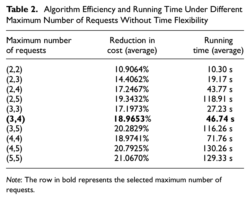
Note: The row in bold represents the selected maximum number of requests.

We also need to determine the probability of each operator being selected. Therefore, we conduct a sensitivity analysis on the probability of operator selection and record the percentage (pct.) reduction of total cost, the pct. reduction of vehicle miles traveled (VMT) and the running time. The results are shown in Figures 9 to 11, where “p1” denotes the probability that the Shaw removal is selected and “p2” denotes the probability that the greedy insertion is selected. From Figures 9 to 11, we can observe that the operator selection probability has little impact on the running time, but has a great impact on the algorithm effect. The largest pct. reductions of total cost and VMT occur when Shaw removal has a selection probability of 0.7 and greedy insertion has a selection probability of 0.9. The following experiments are carried out under this setting.

Figure 9.

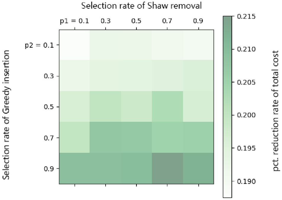
Percentage reduction of total cost under different probability of operator selection.

Figure 10.

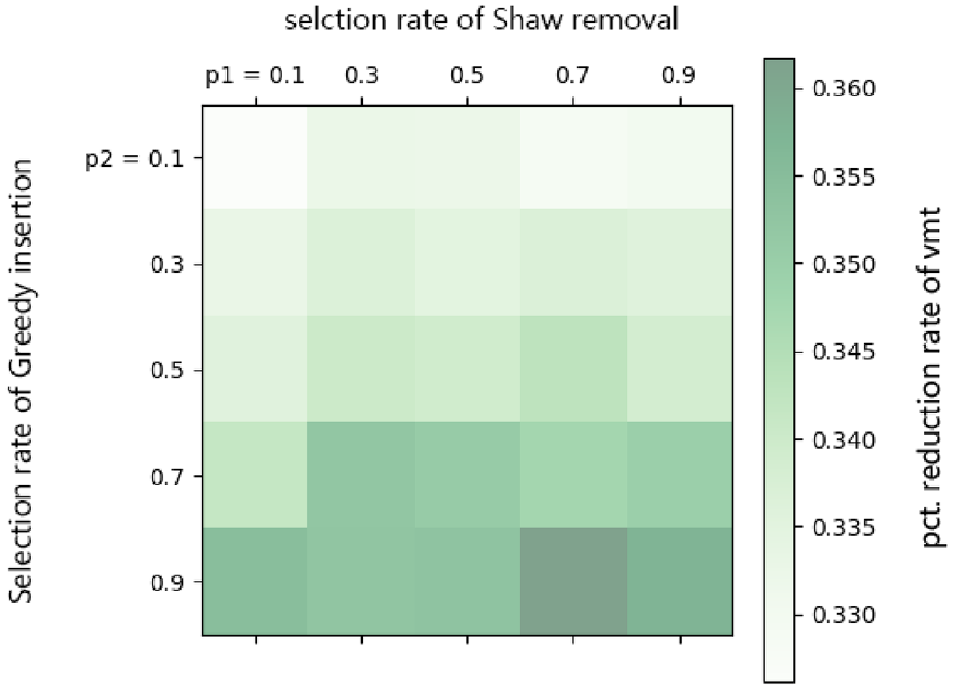
Percentage reduction of vehicle miles traveled (VMT) under different probability of operator selection.

Figure 11.

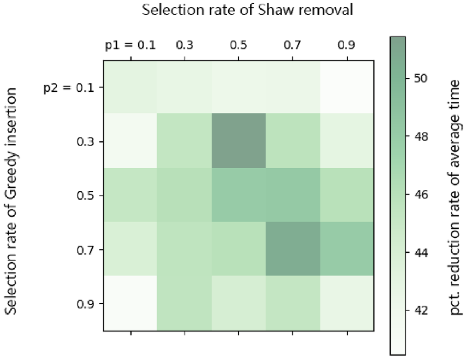
Running time of re-optimization under different probability of operator selection.

Main Results

In this section, we perform cargo pooling in on-demand ICFL. The detailed results of each small time period are shown in the Table 3. The table lists the results of each static cargo pooling, including the number of requests received, cost of distance with and without cargo pooling, penalty for late delivery with and without cargo pooling, number of reloading, total cost with and without cargo pooling, VMT with and without cargo pooling, percentage of total cost reduction and percentage of VMT reduction.

Table 3.

Detailed Results of Each Small Time Period Without Time Flexibility

Time	N	Cost of distance (CD)		Penalty for late delivery (PLD)		Total cost (TC)				Vehicle miles traveled (VMT)
Time	N	CD1	CD2	PLD1	PLD2	NR	TC1	TC2	CRR	VMT1	VMT2	VMT_RR	Running time (Seconds)
08:00	65	2104.1	1583.2	13.7	349.7	11	2117.8	1943.9	8.2%	1502.9	1130.8	24.8%	19.77
08:10	83	2483.8	1821.9	0.0	358.1	19	2483.8	2198.9	11.5%	1774.1	1301.3	26.7%	28.96
08:20	138	5213.8	3936.6	9.1	897.2	27	5222.9	4860.8	6.9%	3724.1	2811.8	24.5%	41.10
08:30	139	4970.5	3453.3	8.0	781.7	34	4978.6	4269.0	14.3%	3550.4	2466.6	30.5%	34.82
08:40	175	5613.2	3590.2	41.9	915.1	30	5655.1	4535.3	19.8%	4009.4	2564.4	36.0%	43.81
08:50	168	6543.4	4799.9	33.8	976.7	40	6577.2	5816.6	11.6%	4673.9	3428.5	26.6%	41.77
09:00	198	7208.5	4918.5	36.1	949.3	56	7244.6	5923.7	18.2%	5148.9	3513.2	31.8%	43.94
09:10	211	6775.7	4332.5	25.7	1004.1	45	6801.4	5381.6	20.9%	4839.8	3094.6	36.1%	64.61
09:20	215	7449.6	4664.7	0.2	927.8	50	7449.8	5642.5	24.3%	5321.2	3331.9	37.4%	66.44
09:30	280	10334.7	6675.3	30.2	1491.6	62	10364.9	8228.9	20.6%	7381.9	4768.1	35.4%	41.82
09:40	226	7581.7	4929.3	18.0	1170.2	49	7599.7	6148.5	19.1%	5415.5	3520.9	35.0%	30.75
09:50	251	8886.7	5515.9	30.5	1322.4	53	8917.3	6891.3	22.7%	6347.7	3939.9	37.9%	44.10
10:00	286	10035.7	6142.2	10.7	1478.8	75	10046.3	7696.0	23.4%	7168.3	4387.3	38.8%	66.15
10:10	282	10795.4	6392.8	4.4	1477.8	93	10799.8	7963.6	26.3%	7711.0	4566.3	40.8%	33.95
10:20	259	8762.2	5429.0	42.9	1316.6	55	8805.2	6800.6	22.8%	6258.7	3877.9	38.0%	40.74
10:30	269	9844.9	6023.9	17.4	1445.3	64	9862.3	7533.2	23.6%	7032.1	4302.8	38.8%	41.06
10:40	275	9816.5	6293.2	18.3	1447.5	59	9834.9	7799.8	20.7%	7011.8	4495.2	35.9%	65.58
10:50	252	8312.0	5566.3	56.9	1459.4	45	8368.9	7070.7	15.5%	5937.1	3976.0	33.0%	57.74
11:00	259	9631.0	6280.5	8.4	1419.0	63	9639.4	7762.6	19.5%	6879.3	4486.1	34.8%	72.01
11:10	217	7046.5	4452.1	8.7	1319.1	43	7055.1	5814.2	17.6%	5033.2	3180.0	36.8%	43.05
11:20	218	7849.5	5165.0	33.3	1251.2	45	7882.8	6461.2	18.0%	5606.8	3689.3	34.2%	43.98
11:30	180	5724.3	4562.9	12.8	956.0	27	5737.1	5545.8	3.3%	4088.8	3259.2	20.3%	10.15
11:40	193	6367.9	4446.3	46.1	1145.5	33	6414.0	5624.7	12.3%	4548.5	3175.9	30.2%	36.11
11:50	178	6227.9	4094.0	19.1	1203.2	41	6246.9	5338.2	14.5%	4448.5	2924.3	34.3%	37.57
12:00	199	6928.9	4889.0	30.3	1344.8	46	6959.1	6279.8	9.8%	4949.2	3492.1	29.4%	59.00
12:10	181	6781.4	4954.5	18.0	1093.6	26	6799.4	6074.1	10.7%	4843.9	3538.9	26.9%	60.06
12:20	203	6573.0	4440.2	23.0	1159.0	43	6596.0	5642.2	14.5%	4695.0	3171.6	32.4%	59.80
12:30	230	8178.6	4986.8	51.3	1465.0	56	8230.0	6507.9	20.9%	5841.9	3562.0	39.0%	23.34
12:40	255	9632.8	5969.0	11.6	1324.1	82	9644.5	7375.1	23.5%	6880.6	4263.6	38.0%	51.26
12:50	285	10773.9	6944.1	26.6	1847.0	57	10800.5	8848.1	18.1%	7695.7	4960.0	35.5%	29.79
13:00	296	11013.3	6674.4	25.8	1491.3	57	11039.0	8222.6	25.5%	7866.6	4767.4	39.4%	68.20
13:10	288	11166.1	7788.4	26.6	1707.6	64	11192.7	9560.1	14.6%	7975.8	5563.2	30.2%	32.63
13:20	297	10385.8	6512.4	15.8	1521.9	53	10401.6	8087.3	22.2%	7418.4	4651.7	37.3%	31.58
13:30	323	12645.8	8070.0	12.3	1719.4	82	12658.1	9871.5	22.0%	9032.7	5764.3	36.2%	61.6
13:40	325	11766.2	7475.7	57.5	1850.2	96	11823.7	9421.8	20.3%	8404.4	5339.8	36.5%	57.04
13:50	317	13120.8	7943.3	24.8	1743.1	88	13145.6	9774.4	25.6%	9372.0	5673.8	39.5%	47.64
14:00	361	12451.3	7356.2	22.1	1464.9	94	12473.5	8915.1	28.5%	8893.8	5254.4	40.9%	39.38
14:10	320	12457.3	7717.0	7.7	1436.5	109	12465.0	9262.5	25.7%	8898.1	5512.1	38.1%	94.93
14:20	361	13981.2	8271.8	43.5	1636.0	106	14024.7	10013.7	28.6%	9986.5	5908.4	40.8%	75.89
14:30	327	13015.8	7909.9	33.2	1513.4	76	13049.0	9499.2	27.2%	9297.0	5649.9	39.2%	60.65
14:40	300	11048.6	6767.8	12.6	1565.0	85	11061.2	8417.8	23.9%	7891.8	4834.2	38.7%	52.12
14:50	335	13509.4	8169.7	10.7	1866.7	97	13520.1	10133.4	25.0%	9649.6	5835.5	39.5%	41.12
15:00	325	10306.6	6061.7	26.2	1515.7	75	10332.9	7652.4	25.9%	7361.9	4329.8	41.2%	94.63
15:10	332	12489.2	8801.5	21.4	1758.4	74	12510.5	10633.9	15.0%	8920.8	6286.8	29.5%	72.20
15:20	375	14359.5	8811.6	12.7	1646.3	108	14372.2	10565.9	26.5%	10256.8	6294.0	38.6%	87.78
15:30	313	12033.8	7563.3	5.0	1440.0	83	12038.9	9086.3	24.5%	8595.6	5402.4	37.1%	67.64
15:40	304	11839.9	7560.4	32.5	1498.0	87	11872.4	9145.4	23.0%	8457.0	5400.3	36.1%	76.96
15:50	323	12164.8	7957.1	21.6	1489.9	76	12186.4	9523.0	21.9%	8689.1	5683.6	34.6%	36.56
16:00	304	10422.4	6105.5	41.9	1345.3	89	10464.3	7539.8	27.9%	7444.6	4361.1	41.4%	47.52
16:10	330	11503.4	6653.6	17.3	1374.3	114	11520.8	8142.0	29.3%	8216.7	4752.6	42.2%	30.64
16:20	291	11004.6	6763.4	0.4	1221.8	84	11005.0	8069.3	26.7%	7860.4	4831.0	38.5%	30.38
16:30	260	10014.9	6184.7	2.2	1083.8	67	10017.2	7335.5	26.8%	7153.5	4417.6	38.2%	60.72
16:40	271	9798.5	6600.7	27.5	1074.5	51	9826.0	7726.2	21.4%	6998.9	4714.8	32.6%	34.29
16:50	267	9698.9	5844.7	0.1	828.7	65	9699.0	6738.3	30.5%	6927.8	4174.8	39.7%	49.26
17:00	251	9458.3	5944.4	12.6	1117.1	63	9470.9	7124.4	24.8%	6755.9	4246.0	37.2%	56.25
17:10	208	7264.2	4685.7	14.9	928.7	29	7279.1	5643.5	22.5%	5188.7	3346.9	35.5%	27.84
17:20	204	7307.6	4542.3	0.0	917.1	59	7307.6	5518.4	24.5%	5219.7	3244.5	37.8%	60.25
17:30	184	6579.9	4111.1	8.5	647.2	40	6588.4	4798.3	27.2%	4699.9	2936.5	37.5%	16.75
17:40	153	4652.3	3082.1	11.6	561.0	24	4663.8	3667.1	21.4%	3323.0	2201.5	33.7%	95.95
17:50	139	4330.9	2883.9	12.7	761.9	30	4343.6	3675.9	15.4%	3093.5	2059.9	33.4%	19.81
18:00	138	4374.1	2728.2	0.0	753.0	25	4374.1	3506.2	19.8%	3124.3	1948.7	37.6%	46.39
18:10	98	3268.2	2312.0	0.0	526.0	15	3268.2	2853.1	12.7%	2334.5	1651.5	29.3%	36.68
18:20	108	2614.0	1895.8	4.3	515.4	9	2618.3	2420.2	7.6%	1867.2	1354.1	27.5%	31.55
18:30	78	2313.2	1607.2	1.8	330.2	6	2315.1	1943.4	16.1%	1652.3	1148.0	30.5%	30.68
18:40	100	3102.2	1964.0	9.9	541.9	17	3112.1	2522.9	18.9%	2215.8	1402.9	36.7%	24.16
18:50	73	2326.8	1696.9	22.2	518.8	15	2348.9	2230.8	5.0%	1662.0	1212.1	27.1%	26.53
19:00	79	1542.0	1091.0	9.2	407.7	8	1551.2	1506.7	2.9%	1101.4	779.3	29.3%	27.26

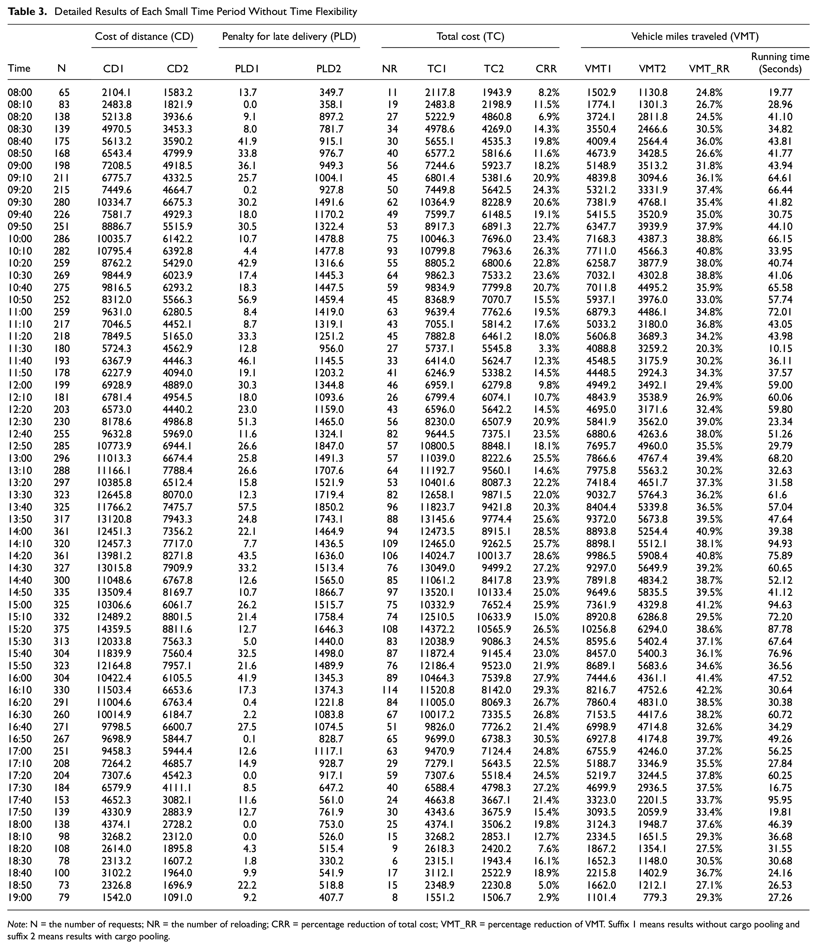
Note: N = the number of requests; NR = the number of reloading; CRR = percentage reduction of total cost; VMT_RR = percentage reduction of VMT. Suffix 1 means results without cargo pooling and suffix 2 means results with cargo pooling.

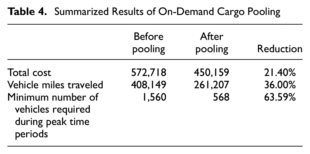
A summary of the results in Table 3 is shown in Table 4. We extracted some parameters that are of most interest in this study, including total cost with and without cargo pooling, percentage of cost reduction, VMT with and without cargo pooling, percentage of VMT reduction and minimum number of vehicles required with and without cargo pooling. The minimum number of vehicles required is equal to the maximum number of vehicles used to fulfill all delivery requests across all periods.

Table 4.

Summarized Results of On-Demand Cargo Pooling

	Before pooling	After pooling	Reduction
Total cost	572,718	450,159	21.40%
Vehicle miles traveled	408,149	261,207	36.00%
Minimum number of vehicles required during peak time periods	1,560	568	63.59%

To better quantify the value of cargo pooling for on-demand city logistics, we divide the results in Table 3 into peak periods and off-peak periods, and check the value of cargo pooling at the two time periods respectively. If the number of requests arriving within 10 min is greater than 250, this period is called peak period. If not, it is called off-peak period. The results are summarized in Table 5. The average NR denotes the average number of reloading.

Table 5.

Results in Peak Periods and Off-Peak Periods

	Before pooling	After pooling	pct. reduction
Peak period
Total cost	399255	304432	23.75%
VMT	284630	177673	37.58%
Average NR	na	76.4	na
Off-peak period
Total cost	167,822	140,295	19.23%
VMT	119,498	80,443	32.68%
Average NR	na	32.2	na

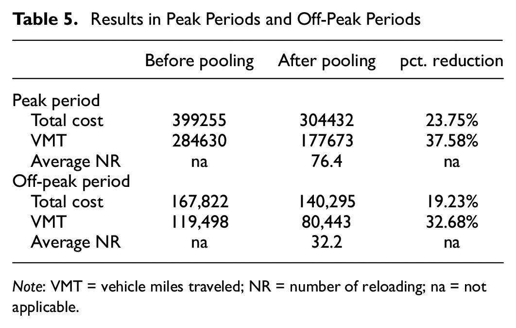
Note: VMT = vehicle miles traveled; NR = number of reloading; na = not applicable.

We also compare situations where we allow reloading in the problem versus when we offer LIFO and no reloading. The results are shown in Table 6.

Table 6.

Comparison Between LIFO and Reloading

	Total cost			Vehicle miles traveled
	Before pooling	After pooling	Reduction	Before pooling	After pooling	Reduction
LIFO	572,718	453,936	20.74%	408,149	281,829	30.95%
Reloading		450,159	21.40%		261,207	36.00%

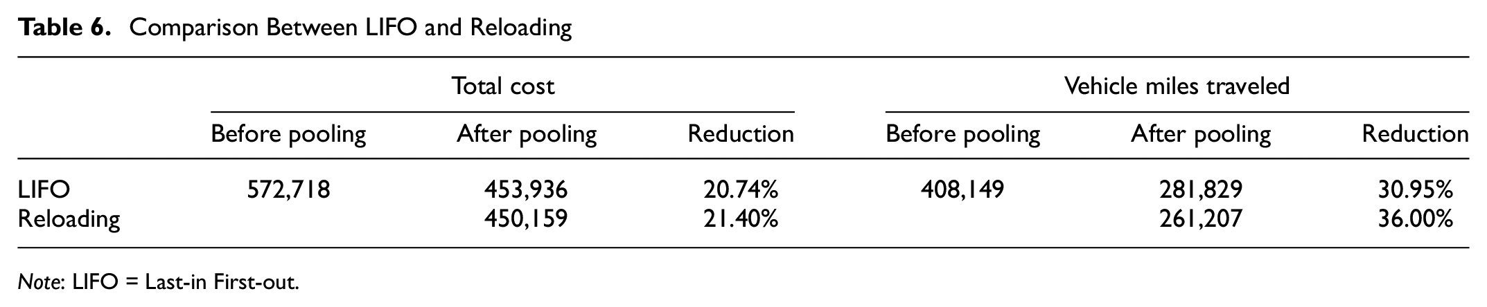
Note: LIFO = Last-in First-out.

Analysis of Main Results

Based on Tables 3 and 4, it is evident that cargo pooling results in significant reductions in both daily cost (21.40%) and VMT (36%). These findings demonstrate that cargo pooling can effectively reduce the cost of logistics companies in on-demand ICFL, as compared with the traditional point-to-point service model. Furthermore, the traditional model would require at least 1,560 vehicles to fulfill all requests during peak periods, whereas cargo pooling reduced this number to 568, thereby increasing supply during high demand periods. These improvements highlight the substantial benefits of cargo pooling over the traditional point-to-point service model in on-demand ICFL. Consequently, for logistics companies with high business volumes, cargo pooling can help meet more requests, reduce costs, and maintain competitiveness in the on-demand ICFL market.

According to Table 5, cargo pooling results in a 19.23% reduction in total cost during off-peak periods, while during peak periods it can reduce total cost by 23.75%. These findings demonstrate that the greater the number of requests, the more significant the total cost reduction achieved through cargo pooling. A similar trend is observed for VMT reduction, with cargo pooling reducing VMT by 32.68% during off-peak periods and 37.58% during peak periods. This is because a larger number of requests provides more opportunities for request consolidation, enabling more efficient cargo pooling. This principle underscores the importance of cargo pooling for rapidly growing or large logistics companies that receive a significant volume of on-demand requests.

It can be seen from Table 6 that cargo pooling with LIFO can reduce VMT by 30.95%. But cargo pooling with reloading can reduce VMT by 36.00%, which is much bigger. As for the total cost reduction, the difference between the two situations is not significant. The differences between the situation with LIFO and with reloading are: (i) the LIFO rule limits the freedom of path choice, so the VMT in the situation with LIFO will be longer; (ii) allowing reloading will cause extra labor cost and longer staying time. The experimental results are in line with our expectations. The pct. reduction of VMT in the reloading situation is 30.95%, which is less than the 36.00% reduction of VMT in the LIFO situation. But with the extra labor cost and penalty for late delivery caused by longer staying time, the pct. reductions of total cost in these two situations, 20.74% and 21.40%, show little difference. This presents logistics companies with the option of whether to permit reloading. The ideal choice will depend on factors such as the company’s staff salary level and other relevant considerations, which should be determined through simulation.

Sensitivity Analysis on Time Flexibility

In this section, we experiment with on-demand cargo pooling under different levels of time flexibility. As introduced before, we adjust the time flexibility through extending the time windows of delivery. We choose 10 min, 20 min, and 30 min as three different levels of time flexibility.

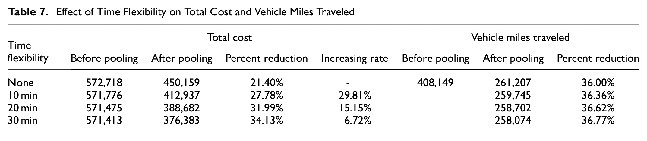
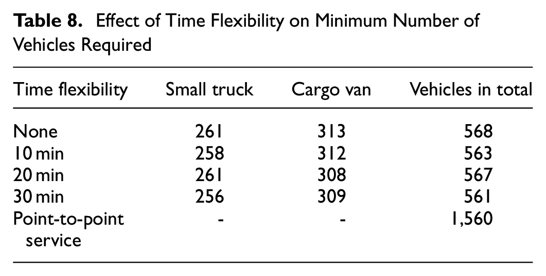
A summary of the on-demand cargo pooling under different levels of time flexibility is shown in Table 7. Except for the increasing rate of pct. of cost reduction when time flexibility increases, other parameters are the same as in Table 4. It can be seen that the total cost reduction can increase with the increase of the level of time flexibility. But as the level of time flexibility increases, the increase in cost reduction gradually becomes slower, from 29.81% to 15.15% and 6.72%. This means that there is a saturation threshold for time flexibility, which means the maximum of the delay caused by cargo pooling. As introduced at the beginning of this paper, cargo pooling is a way to reduce total cost and total VMT by extending the delivery time of a single request. Adding time flexibility can reduce the impact of extended time on a single request. Sensitivity analysis for time flexibility can help logistics companies better assess the reduced customer experience and cost reduction brought about by cargo pooling. However, it is difficult to reduce VMT by time flexibility, and it is the stable optimization of the logistics system by cargo pooling. Furthermore, the impact of time flexibility on the minimum number of vehicles required is shown in Table 8. The reduction in minimum number of vehicles required is also stable as time flexibility changes. It is worth mentioning that the minimum number of small trucks required plus the minimum number of cargo vans required is larger than the minimum number of vehicles required in total. This is because of $\max {A} + \max {B} \leq \max {A + B}$ , which makes sense.

Table 7.

Effect of Time Flexibility on Total Cost and Vehicle Miles Traveled

Time flexibility	Total cost				Vehicle miles traveled
Time flexibility	Before pooling	After pooling	Percent reduction	Increasing rate	Before pooling	After pooling	Percent reduction
None	572,718	450,159	21.40%	-	408,149	261,207	36.00%
10 min	571,776	412,937	27.78%	29.81%		259,745	36.36%
20 min	571,475	388,682	31.99%	15.15%		258,702	36.62%
30 min	571,413	376,383	34.13%	6.72%		258,074	36.77%

Table 8.

Effect of Time Flexibility on Minimum Number of Vehicles Required

Time flexibility	Small truck	Cargo van	Vehicles in total
None	261	313	568
10 min	258	312	563
20 min	261	308	567
30 min	256	309	561
Point-to-point service	-	-	1,560

Conclusion and Future Work

In this study, we aim to address the issue of vehicle shortage during high demand periods by investigating the benefits of cargo pooling in on-demand ICFL. We establish a dynamic PDP with 3D-Loading and time window constraints for cargo pooling in on-demand ICFL and develop a dynamic algorithm for the solution. Through a simulation experiment utilizing real-world freight data, we demonstrate that cargo pooling can significantly reduce both the distance traveled by cargo vans and the overall cost. Additionally, we examine the effect of varying levels of delivery time flexibility and find that while time flexibility has a significant impact on cost reduction, it has a minimal effect on total VMT. Our research provides valuable insights for logistics companies in determining the value of cargo pooling and can serve as a reference for their cargo pooling practices.

However, our research still has some limitations. In our future research, we will improve our model in the following aspects:

We will develop a predictive model and take the randomness of requests into consideration. In each optimization period, we will experiment with cargo pooling with historical requests, newly arrived requests, and predicted requests.

Our static part is modeled as 3L-PDPTW, which takes a long time to solve. We do not take into account the running time of the program in this paper. In practice, new requests and routes can only be assigned to vehicles after the program has finished running. And within these minutes, the states of the vehicles and the requests may also change.

In this study, we assume that all customers accept the cargo pooling service. In the future, we will model a shipper’s choice between cargo pooling and conventional point-to-point service and develop a hybrid cargo pooling model.

Besides the model limitations, logistics companies are also faced with some barriers to implement the cargo pooling in on-demand ICFL:

1. Since the dimensions of cargoes can be irregular, it can be difficult for shippers to describe the cargo sizes adequately and accurately, which may lead to failure of the cargo pooling exercise in practice;

2. There is risk of cargoes being taken out by mistake or broken when reloading;

3. Not all customers are willing to accept cargo pooling—the platform needs to offer a choice between cargo pooling and standard service;

4. In current operations, there is no punishment to the driver if late delivery occurs;the pricing strategy needs more research.

Footnotes

Author Contributions

The authors confirm contribution to the paper as follows: study conception and design: S. Cao, H. Jiang; data collection: Z. Lei, L. Zhao, S. Cao; analysis and interpretation of results: Z. Lei, H. Jiang, S. Cao, L. Zhao; draft manuscript preparation: Z. Lei, H. Jiang. All authors reviewed the results and approved the final version of the manuscript.

Declaration of Conflicting Interests

The author(s) declared no potential conflicts of interest with respect to the research, authorship, and/or publication of this article.

Funding

The author(s) disclosed receipt of the following financial support for the research, authorship, and/or publication of this article: This project is funded by the National Natural Science Foundation of China under grant no. 72361137005 and by Tsinghua University-DiDi Joint Research Center for Future Mobility.

ORCID iDs

Hai Jiang

Shaosheng Cao

References

Report of Market Prospects and Investment Strategy Planning Analysis on China Logistics Industry (2022-2027). FORWARD Business Information Co., Ltd., Shenzhen China, 2022.

Montoya-Torres

J. R.

Muñoz-Villamizar

Vega-Mejía

C. A.

On the Impact of Collaborative Strategies for Goods Delivery in City Logistics. Production Planning & Control, Vol. 27, No. 6, 2016, pp. 443–455.

Pan

Ballot

Fontane

The Reduction of Greenhouse Gas Emissions from Freight Transport by Pooling Supply Chains. International Journal of Production Economics, Vol. 143, No. 1, 2013, pp. 86–94.

Kay

M. G.

Karagul

Sahin

Aydemir

Shipment Consolidation Practice Using Matlog and Large-Scale Data Sets. In Smart Applications with Advanced Machine Learning and Human-Centred Problem Design ( Hemanth

D. J.

Kose

Watada

Patrut

, eds.), Springer, Cham, Switzerland, 2023, pp. 701–717.

Männel

Bortfeldt

A Hybrid Algorithm for the Vehicle Routing Problem with Pickup and Delivery and Three-Dimensional Loading Constraints. European Journal of Operational Research, Vol. 254, No. 3, 2016, pp. 840–858.

Männel

Bortfeldt

Solving the Pickup and Delivery Problem with Three-Dimensional Loading Constraints and Reloading Ban. European Journal of Operational Research, Vol. 264, No. 1, 2018, pp. 119–137.

Zheng

Huang

Cai

Feng

Zhang

An Improved Hybrid Heuristic Algorithm for Pickup and Delivery Problem with Three-Dimensional Loading Constraints. Proc., IEEE 31st International Conference on Tools with Artificial Intelligence (ICTAI), Portland, OR, IEEE, New York, 2019, pp. 1607–1612.

Dupas

Grebennik

Lytvynenko

Baranov

An Heuristic Approach to Solving the One-to-One Pickup and Delivery Problem with Three-Dimensional Loading Constraints. International Journal of Information Technology and Computer Science, Vol. 9, No. 10, 2017, pp. 1–12.

Stamadianos

Marinaki

Matsatsinis

Marinakis

A DSS for the Multi-Criteria Vehicle Routing Problem with Pickup and Delivery and 3D Constraints. In Decision Support Systems XII: Decision Support Addressing Modern Industry, Business, and Societal Needs ( Cabral Seixas Costa

A. P.

Papathanasiou

Jayawickrama

Kamissoko

, eds.), Springer International Publishing, Cham, 2022, pp. 177–189.

10.

Gendreau

Iori

Laporte

Martello

A Tabu Search Algorithm for a Routing and Container Loading Problem. Transportation Science, Vol. 40, No. 3, 2006, pp. 342–350.

11.

Bortfeldt

Homberger

Packing First, Routing Second—A Heuristic for the Vehicle Routing and Loading Problem. Computers & Operations Research, Vol. 40, No. 3, 2013, pp. 873–885.

12.

Reil

Bortfeldt

Mönch

Heuristics for Vehicle Routing Problems with Back-Hauls, Time Windows, and 3D Loading Constraints. European Journal of Operational Research, Vol. 266, No. 3, 2018, pp. 877–894.

13.

Moura

A Model-Based Heuristic to the Vehicle Routing and Loading Problem. International Transactions in Operational Research, Vol. 26, No. 3, 2019, pp. 888–907.

14.

Lim

A Metaheuristic for the Pickup and Delivery Problem with Time Windows. International Journal on Artificial Intelligence Tools, Vol. 12, No. 2, 2003, pp. 173–186.

15.

Ahkamiraad

Wang

Capacitated and Multiple Cross-Docked Vehicle Routing Problem with Pickup, Delivery, and Time Windows. Computers & Industrial Engineering, Vol. 119, 2018, pp. 76–84.

16.

Wang

Guan

Fan

Wang

Collaborative Multi-Depot Pickup and Delivery Vehicle Routing Problem with Split Loads and Time Windows. Knowledge-Based Systems, Vol. 231, 2021, p. 107412.

17.

Sitek

Wikarek

Rutczyńska-Wdowiak

Bocewicz

Banaszak

Optimization of Capacitated Vehicle Routing Problem with Alternative Delivery, Pick-Up and Time Windows: A Modified Hybrid Approach. Neurocomputing, Vol. 423, 2021, pp. 670–678.

18.

Luo

Zhang

Yin

Zhu

Qiu

Distribution Vehicle Routing Optimization Based on 3D Loading. In Advances in Smart Vehicular Technology, Transportation, Communication and Applications ( Wu

T.-Y.

Chu

S.-C.

Chen

C.-H.

Favorskaya

, eds.), Springer, Singapore, 2022, pp. 87–97.

19.

Antoniou

Jiang

Xie

Shen

Han

The Value of Prepositioning in Smartphone-Based Vanpool Services Under Stochastic Requests and Time-Dependent Travel Times. Transportation Research Record: Journal of the Transportation Research Board, 2019. 2673: 26–37.

20.

Ropke

Pisinger

An Adaptive Large Neighborhood Search Heuristic for the Pickup and Delivery Problem with Time Windows. Transportation Science, Vol. 40, No. 4, 2006, pp. 455–472.

21.

Bent

Van Hentenryck

A Two-Stage Hybrid Algorithm for Pickup and Delivery Vehicle Routing Problems with Time Windows. Computers & Operations Research, Vol. 33, No. 4, 2006, pp. 875–893.

22.

Lim

A Metaheuristic for the Pickup and Delivery Problem with Time Windows. Proc., 13th IEEE International Conference on Tools with Artificial Intelligence, ICTAI 2001, Dallas, TX, IEEE, New York, 2001, pp. 160–167.

23.

Chen

Lee

S.-M.

Shen

An Analytical Model for the Container Loading Problem. European Journal of Operational Research, Vol. 80, No. 1, 1995, pp. 68–76.

24.

Mitrović-Minić

Laporte

The Pickup and Delivery Problem with Time Windows and Transshipment. INFOR: Information Systems and Operational Research, Vol. 44, No. 3, 2006, pp. 217–227.

25.

Masson

Lehuédé

Péton

An Adaptive Large Neighborhood Search for the Pickup and Delivery Problem with Transfers. Transportation Science, Vol. 47, No. 3, 2013, pp. 344–355.

26.

The Regulation on the Implementation of the Road Traffic Safety Law of the People’s Republic of China. State Council of the People’s Republic of China, 2004, chap. 62, p. 7.

27.

Shaw

Using Constraint Programming and Local Search Methods to Solve Vehicle Routing Problems. Proc., Principles and Practice of Constraint Programming—CP98: 4th International Conference, CP98, October 26–30, 1998, Pisa, Italy. Springer, Berlin, Heidelberg, 1998, pp. 417–431.

28.

Chen

Wang

G.-G.

Gao

Sangaiah

A. K.

An Adaptive Large Neighborhood Search Heuristic for Dynamic Vehicle Routing Problems. Computers & Electrical Engineering, Vol. 67, 2018, pp. 596–607.