
Abstract
A key aspect of the success of shared-use autonomous mobility systems will be the ability to price rides in real time. As these services become more prevalent, it becomes of high importance to detect shifts in behavior to quickly optimize the system and ensure system efficiency and economic viability. Therefore, (1) pricing algorithms should be able to price rides according to complex underlying demand functions with heterogeneous customers and (2) the algorithm should be able detect nonstationary behavior (e.g., changing customers’ willingness to pay) from its previously learnt decisions and alter its pricing mechanism accordingly. We formulate a dynamic pricing and learning problem as a Markov decision process and subsequently solve it through a reinforcement learning (RL) algorithm, with heterogeneous customers accepting the trip characteristics (price, expected wait time) probabilistically. Insights from a fixed fleet operation of an autonomous private ridesourcing system in Chicago are presented. Given our formulation of the demand model, the algorithm learns in 25 days, increasing revenue by 90% and decreasing customer wait times by 90% compared to day 5. After gathering insights from the RL algorithm and applying optimal static pricing (i.e., a constant specific surge multiplier), we find that RL can achieve near 90% optimality in revenue. The RL algorithm, nevertheless, proves to be robust. Two scenarios are tested where a sudden shock occurs or customers slowly change their willingness to pay, illustrating that RL can quickly adapt its parameters to the situation.
Dynamic pricing emerged as a form of revenue management in the late 1970s, after the deregulation of the airline industry ( 1 ). The main goal of dynamic pricing is to adjust the product price at specific times such that service is allocated to the right customer who is willing to pay, in an attempt to maximize total revenue (a typical objective of for-profit companies). Dynamic pricing also helps address situations in which capacity is limited, which can be resolved by raising the price to reduce demand, also known as market clearing.
Application of dynamic pricing is prevalent in the online retailing sector, airline sector, hospitality sector, and intelligent transportation systems ( 2 , 3 ). More recently, dynamic pricing has emerged in ridesourcing/ridesharing systems (Uber, Lyft) to balance supply and stochastic demand, by using “surge multipliers” that are applied to the base fares at times of high demand. This plays an important role for profit and/or user satisfaction maximization in these systems. In current-day human-driven vehicle systems, dynamic pricing affects both the supply and demand, as drivers are more likely to join the system when higher profit is expected, while customers become less likely to accept rides. Autonomous vehicles (AVs) coupled with ridesharing applications will most likely provide a fixed vehicle fleet ( 4 ) that safely and efficiently traverses the road infrastructure, picks up passengers, drops them off without the hassle of looking for parking spots, and engages in the same activity repeatedly—defined as shared-use autonomous mobility systems (SAMSs).
A key aspect of the success of these autonomous systems will be the ability to price rides in real time. Moreover, as these services become more prevalent, it becomes of high importance to detect shifts in behavior to quickly optimize the system and ensure high profitability and good system efficiency. Specifically, (1) pricing algorithms should be able to price rides according to complex underlying demand functions with heterogeneous sensitivities and (2) the algorithm should be able to detect nonstationary behavior (i.e., when the true value of actions changes over time [ 5 ], e.g., because of changing customers’ willingness to pay) from its previously learnt decisions and alter its pricing mechanism accordingly. Thus, the main objectives of this study are as follows.
Formulate a dynamic pricing and learning problem as a Markov decision process (MDP) and subsequently solve it through a reinforcement learning (RL) algorithm, with heterogeneous customers accepting the trip characteristics (price, expected wait time) probabilistically. The RL algorithm will be developed such that it supports continuous actions (i.e., surge multipliers), which is a novel methodology used for continuous problems ( 5 ). Policies will be formulated using a Gaussian parametrization that depends on the state of the system.
Derive insights from fixed fleet operation of an autonomous private ridesourcing system, with respect to the following questions. Does dynamic pricing help with system efficiency and customer service metrics? Does it increase profit compared to optimal static pricing? Can the algorithm learn in nonstationary environments? This will provide evidence as to the robustness of the algorithm compared to static pricing.
Literature Review
Dynamic pricing has been tackled in a variety of methodologies. Queueing approaches and mathematical analysis have been prevalent, but recently, computer scientists have been implementing machine learning methods. Unlike mathematical analysis that attempts to find closed-form solutions (which require many assumptions), computer scientists typically use simulation to update model parameters and optimize specific objective functions. This is the case with RL, a class of algorithms that obtain optimal policies through exploration and exploitation. Three research areas/communities have contributed to modern RL, as documented by Sutton and Barto ( 5 ). The first originated in the psychology of animal behavior, concerning learning through trial-and-error. The second is the study of optimal control, mainly through dynamic programming techniques originated by Richard Bellman. Bellman also originated the discrete stochastic version of optimal control called a MDP. The MDP framework has been used for dynamic pricing by many researchers ( 6 , 7 ) Dynamic programming techniques are governed by a backwards induction formula that goes backwards in time to find an optimal solution, in a fully known environment and with known transition probabilities. This was therefore hard to consider as a learning process in a forward-going process ( 5 ). The third research area is temporal difference learning by adjusting predictions to match later predictions about the future before the final outcome is known. Recently, there have been many advancements in the field, such as policy-gradient methods, Q-learning, average-reward formulations, deep Q-learning, and actor–critic methods. These algorithms use combined knowledge from all three research areas.
A fundamental work in ridesourcing is that done by Banerjee et al. ( 8 ), who formulate the problem of two-sided ridesharing platforms as a stochastic model that captures the dynamics of drivers and passengers. Specifically, the authors model the system as a continuous-time queuing process and analytically present equations of equilibrium that captures the likelihood of drivers to join and riders accepting a ride. The two-queue system is modeled using state-dependent (price-dependent) service rates, referred to as an M/M(k)/1 queue, where the service rate of passengers depends on the current number of available drivers. The authors impose dynamic pricing based on thresholds, whereby a high price is offered to passengers if the number of drivers is less than that threshold, and a lower price when the number of drivers is greater. Moreover, drivers do not react to instantaneous prices but rather focus on their long-term time-average earnings, which incentivizes their participation. The authors present two results, both under a single region and under large-market limits: (1) unexpectedly, dynamic pricing cannot produce better throughput or revenue than optimal static pricing, but (2) dynamic pricing is more robust to errors in model parameters (e.g., demand rate, driver availability rate, etc.). The authors, however, assume a single demand regime and not a periodically changing demand pattern. Moreover, they assume a rider quits the system if not matched right after requesting a ride. These assumptions and results are a major focus of the current paper, albeit in a SAMS.
Research by Pandit et al. ( 9 ) relaxes the above assumption that drivers only react to long-term average earnings, and instead assumes an instantaneous effect of increasing the price on the driver arrival rate. This assumption is investigated by Uber ( 10 ), which shows potential evidence of driver-partners instantaneously joining the platform because of the increased surge. The authors combine queuing models with a MDP to represent the system, with the state space being the difference between the queue length of drivers and customers. They assume the arrival rate of customers is a decreasing concave function of the price, while that of drivers is increasing. The platform’s goal is to maximize the expected time-averaged revenue, which is determined by a weighted average (by stationary distribution of the Markov chain) of the rate of matching multiplied by the price offered at a state and the distance traveled by a customer. Solving this problem through a value iteration technique, the authors show that dynamic pricing strategies outperform static pricing strategies if drivers and customers react instantaneously to price.
Haliem et al. ( 11 ) study the interconnected decisions of matching, pricing, and dispatching for ridesourcing. Firstly, a heatmap of supply and demand (as well as predicted demand) is inputted to the system. Greedy vehicle-to-customer matching is done of ride requests at time t, with each driver notified of the price of the trip. Vehicles next perform an insertion operation, where they propose a price based on a learnt value function of expected discounted rewards at the ride’s destination using an estimated deep Q-network. Customers then have the ability to reject a ride based on their own utility function. Finally, the authors propose rebalancing the network via a deep Q-network whereby vehicles are dispatched to zones with predicted high demand. The authors’ framework incorporates pricing from the driver’s point of view (e.g., profitability, going to a low demand area), but not from the viewpoint of balancing supply and demand. Moreover, pricing is not the decision process modeled as a RL problem. Rather, the expected discounted reward associated with each move on the map is estimated using a deep Q-network, which drives the price decisions set by the drivers themselves (rather than a central controller) based on a ranking of zones. The authors do not specifically study the effect of dynamic pricing compared to static pricing, but present promising results with respect to customer wait times, profitability, and vehicle utilization.
Recently, Chen et al. ( 12 ) applied RL for spatial-temporal pricing for a ridesourcing platform. They use Didi’s explicit data on a specific day to simulate the availability of drivers and ride orders received. They differentiate between two pricing techniques: (1) a dynamic pricing scheme that offers the same price and wage applied in all zones, and (2) spatial-temporal pricing, which assigns a price and wage at each zone separately from others. The state information they consider are the number of waiting passengers and number of idle vehicles in each region at time step t, and the number of occupied vehicles heading to each region. The authors argue that the above information does not reflect the environment, and suggest adding historical demand information at time step t + 1 to state information, which is a complete information case. However, passengers are not given expected wait times when ordering and demand only reflects the current price. Nevertheless, they assume the customer cancels the ride if not matched within 15 min—an excessively long time for urban mobility applications. The authors also price rides based only on the trip origin location, regardless of destination, rather than applying surge multipliers to the distance and time of the trip. The authors adopt a model-free method called proximal policy optimization (PPO) with the policy defined as a deep neural network that selects actions based on given state information. This is an actor–critic policy-gradient method that supports continuous state-action spaces. The reward is equal to the total revenue minus the driver salary at time step t. The authors show that dynamic pricing could generate 25% more profit compared to static prices, while spatial-temporal pricing could attain up to 85% more profit, but do not provide improvement details for customer wait times.
Surge pricing in traditional ridesourcing systems (human drivers) is distinctly different than in SAMSs. Surge pricing in traditional systems affects both the supply and demand, as it encourages drivers to join the platform and reduces the rider’s probability of accepting a ride. This is not the case when AVs are used; therefore, extracting insights from this system is novel and important. Moreover, the envisioned fixed fleet size is another important difference that needs to be modeled and analyzed.
The closest line of research to this paper was recently conducted by Turan et al. ( 13 ), who seek to optimize a system of electric SAMSs, specifically considering joint routing (assignment to customers and rebalancing), battery charging, and pricing. The authors characterize the network as a fully connected graph where each node corresponds to a zone, which is set as the starting/ending position of rides and the location of charging stations. They model the arrival process between origin–destination (OD) pairs as a Poisson process that is dependent on the current price and consider the operational and charging costs of vehicles. In their model, customers are assigned to a queue for each OD pair and are served on a first-come-first-served basis after being matched. The authors first formulate and solve the “optimal” static problem (average arrival rates, no stochasticity, perfect knowledge of environment parameters) through a network flow model. Next, the authors formulate a real-time policy using RL. The state information that they consider consists of vehicle locations and energy levels, queue lengths at each OD pair, and electricity prices at each node. The actions are the prices for each OD pair and routing/rebalancing/charging decisions for each vehicle. The reward consists of revenue gained by arrivals, queue costs, and operational/charging costs. The authors adopt the model-free method, PPO. They conduct simulations using Manhattan and San Francisco datasets (of only 2 h of a specific day) with Manhattan split into 10 regions and San Francisco split into seven. They show that RL maximizes profit by 10% and minimizes queues by 70% compared to the optimal static problem. The authors took the approach of aggregating trips into zones. The present paper uses disaggregated data with the vehicle-to-customer assignment algorithm explicitly taking into account the distance between them using bipartite matching techniques. This further enables studying the wait times experienced by customers. Moreover, the areas are not divided into zones but rather the entire system is studied such that pricing (the surge multiplier) is determined based on the system state.
Karamanis et al. ( 14 ) also study utility-based dynamic pricing in a SAMS that offers private and pooled trips. The authors assume complete knowledge of the customers’ choice process of the two modes and public transit (i.e., exact probabilities of choosing each), and model it using a nested logit model. Next, the authors apply dynamic pricing by using a surge multiplier (for each customer) that maximizes the expected revenue (probability of private trip choice multiplied by fare + probability of pooled trip choice multiplied by fare). The authors create simulated OD data from data of Greater London and use it to run simulations with varying fleet sizes. However, in their formulation, the authors do not specify how waiting time is calculated for each rider, nor vehicle-to-customer matching details. Interestingly, they find that dynamic prices occur at non-peak times. They show that in a monopoly, dynamic pricing provides a higher revenue than static pricing (however, they do not compare against the optimal static surge multiplier to serve as a fair comparison).
To summarize, compared to previous work, this paper presents a complete framework using a realistic ridesourcing simulator, with details on customer wait times (and learning them), the matching algorithm, and testing of behaviorally challenging scenarios using the developed RL algorithm. Specifically, we use RL to price trips in a fixed fleet system to extract insights. Demand is exogenous, with probabilistic arrivals, and the user decides probabilistically whether to order a ride based on the price and the expected wait time. Matching is also implemented in a microscopic simulator, with the service rate determined through a Manhattan-based grid-road assuming fixed vehicle speed.
Problem Statement
SAMSs consist of a fleet of driverless vehicles serving customer requests. These fleets are likely to be centrally controlled by a single entity in the future. In this paper, the controller operates a fixed fleet whereby user requests come immediately for a point-to-point service. From the customer’s standpoint, the customer opens the app, inputs the pickup and drop-off locations of the trip, and sees the expected wait time and the price. The controller accordingly needs to choose the correct price to maximize system performance (broadly defined). Next, the customer either accepts or rejects the trip, after which the customer joins the queue of customers to be matched to vehicles.
This paper further assumes the following:
users want AVs to come to their pickup location as soon as possible;
the fleet controller cannot reject user requests and users will not cancel trips if wait times are higher than the provided expected wait time;
no en route detours can occur to pick up or drop off other users;
AVs in the fleet are homogeneous;
the fleet size is fixed in the short term;
the fleet controller has complete control over each AV.
The fleet controller has a fleet of AVs
In this paper, we utilize Uber’s pricing strategy in Chicago (Summer 2020). Specifically, the cost of a ride is given as follows:
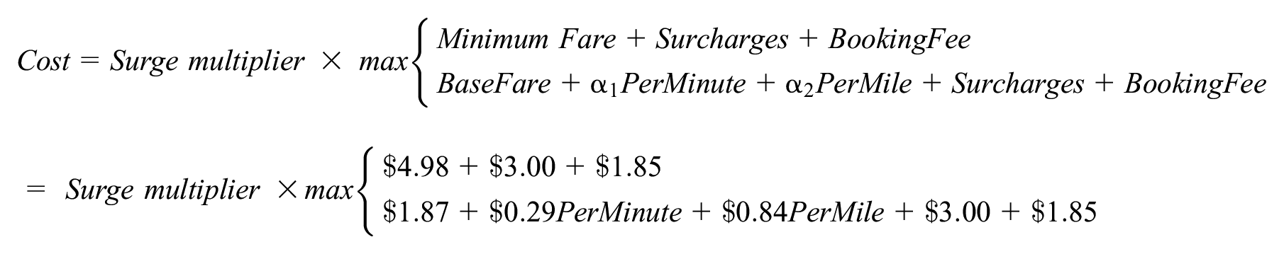
where “surge multiplier” is the action to be learnt online. Moreover, we assume there is a function f through which customers probabilistically accept a ride, based on trip characteristics (e.g., expected wait time and cost). This function could follow any formulation, since, as later shown, the reward function does not use any of its information, but one has to note the algorithm’s performance may change across choice models (e.g., rule-based functions are more challenging to learn). In this paper, we use a mixed logit model that inherently considers the heterogeneity of customers, whereby the systematic utility of accepting a ride is modeled as follows:
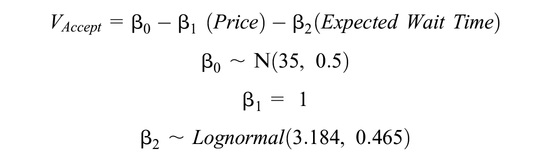
and the systematic utility of not accepting the ride is set to zero. With this formulation, the mean value of wait time is $27/h, and it follows a lognormal distribution. To simulate whether a customer accepts a ride, we draw the coefficients from their respective distributions, compute the systematic utility of accepting, and add to it a random draw from a Gumbel distribution with parameters (0, 1). If this draw is greater than another random draw from a Gumbel distribution with parameters (0, 1), then the customer accepts the ride. Otherwise, they reject the ride.
Model Framework and Online Solution Method
We discuss below the three main algorithms used to drive the simulation. This includes the RL algorithm for pricing (the main objective of this paper), wait time estimation, and matching of vehicles to customers.
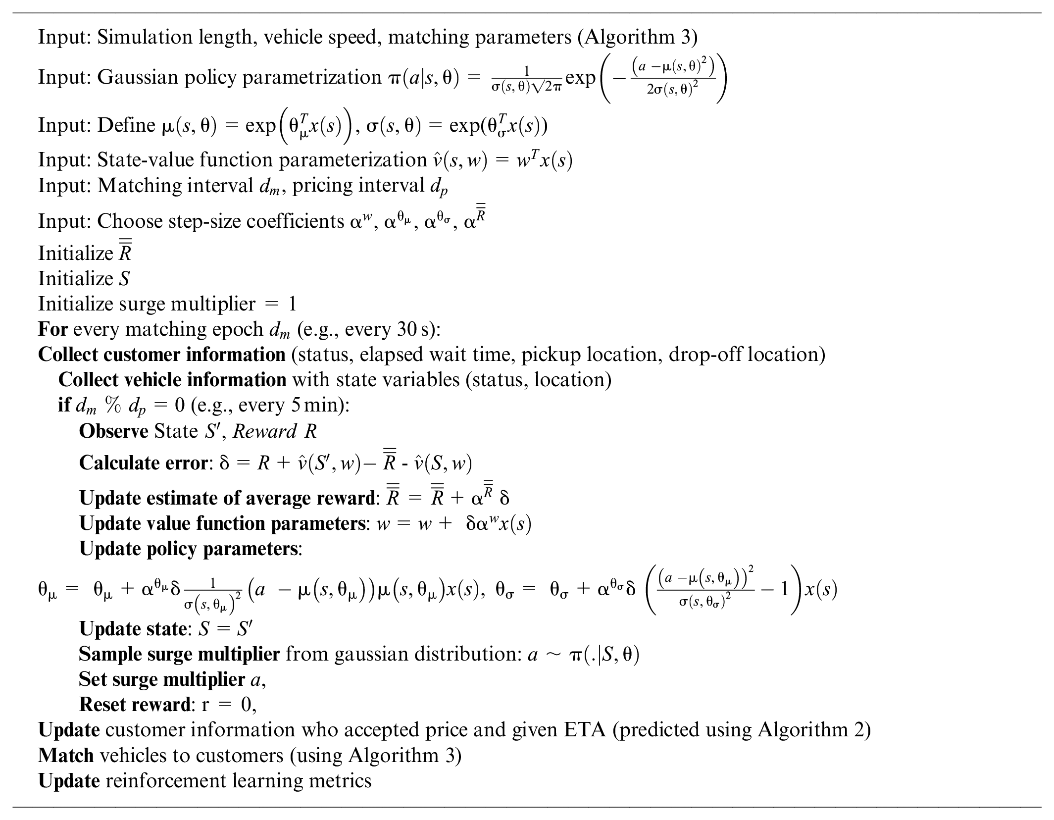
Algorithm 1: Pricing Model Using Reinforcement Learning
The controller is the agent that is trying to learn pricing decisions based on the current state of the system for a specific horizon length (every 5 min in this paper). The MDP contains four elements: a set of states S, a set of actions A, a reward function
State
In this paper, the state of the system is characterized by features
Action
The action to be applied is the surge multiplier. We let the action be global, that is, the same for all OD pairs, but future work can investigate localized pricing. The surge multipliers are modeled to be continuous rather than discrete (see the Solution Methodology section).
Reward
Based on the surge multiplier chosen, the overall reward is the revenue gathered from the customers who accepted the rides. However, because of the time-changing behavior of demand, this is normalized by the number of requests received over the past horizon, that is, the demand:

The reasoning behind this is that the RL algorithm does not realize demand is changing temporally and therefore the reward associated with specific actions may overestimate that action’s importance (e.g., receiving a high reward during a high demand time). This can be fixed by normalizing using the observed demand.
Transition Function
Collect state features (s) from the simulator to find the transition of the state because of the action.
Solution Methodology
We utilize the policy-gradient method with an average-reward formulation ( 5 ). Specifically, we learn a policy (that maps a state to an action) by directly parameterizing the policy, that is:

where a is the action, s is the state, θ represents the parameters of the policy, and t refers to the current time. In this paper, we follow a Gaussian policy parameterization, as follows:
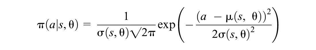
where

where
The policy attempts to maximize the average reward, defined as follows:

The policy-gradient theorem gives an update rule, whereby:
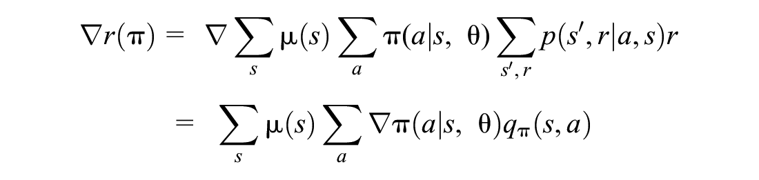
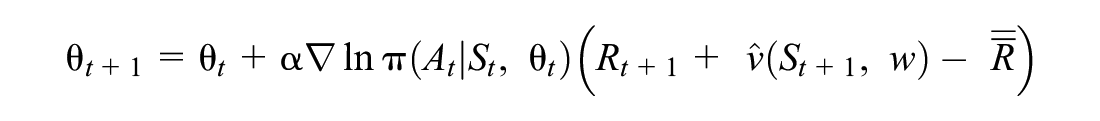
Since the states are generated via policy π, then the stochastic gradient ascent updates policy parameters as follows:

where
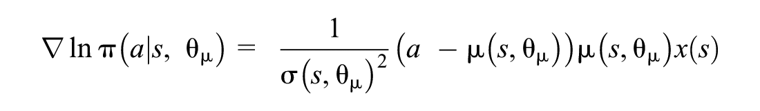
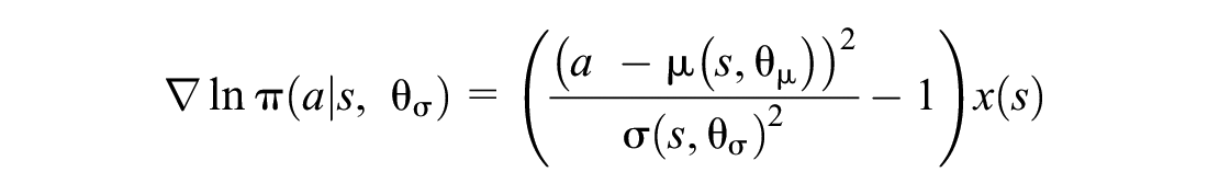
For our selected Gaussian policy, the gradient of the logs are as follows:
We therefore need to approximate
where

We then subtract off a baseline from the temporal difference error to reduce the variance of the update. This is typically chosen as

This algorithm is used continuously (updates every 5 min) with the simulator running continuously as well. Note that we use “episode” and day interchangeably in this paper to refer to a full day of ridesourcing service, but the algorithm does not stop after the end of the day but rather continues on to the next day (and is therefore a continuous problem). This is unlike episodic problems, such as chess.
Algorithm 2: Wait Time Estimation
We utilize a data-based approach to estimate wait times given to customers. After each episode of training, we utilize the following variables for training a linear regression model:
Predictors.
At the time at which the customer requested the ride.
For each non-overlapping surrounding area (see Figure 1, e.g., the blue area), find the following: the number of idle vehicles; the number of non-idle vehicles; the number of unassigned customers;
the number of assigned customers.
Dependent variable: actual wait time of the customer (retrieve once the simulation of the episode is over).
Assume a linear function:

Note that the non-overlapping areas could be set to any dimensions to achieve better predictions; in this paper, we use 1, 2, 6, and 10 mi and infinity. This approach was compared to a prediction based on the nearest vehicle to the customer and achieved lower mean absolute errors (∼3 min). Machine learning methods rather than linear regression will be tested in future work.

Non-overlapping areas for data gathering for wait time estimation (color online only).
Algorithm 3: Matching Vehicles to Customers
We utilize Hyland and Mahmassani’s (
4
) formulated optimization algorithm (Strategy #3) to match idle vehicles (
If the number of unassigned customers is greater than the number of idle vehicles:

where
Subject to the following constraints:


If the number of unassigned customers is less than or equal to the number of unassigned vehicles:

Subject to the following constraints:


Full Simulation Framework
The full simulation framework is described both below and in Figure 2.
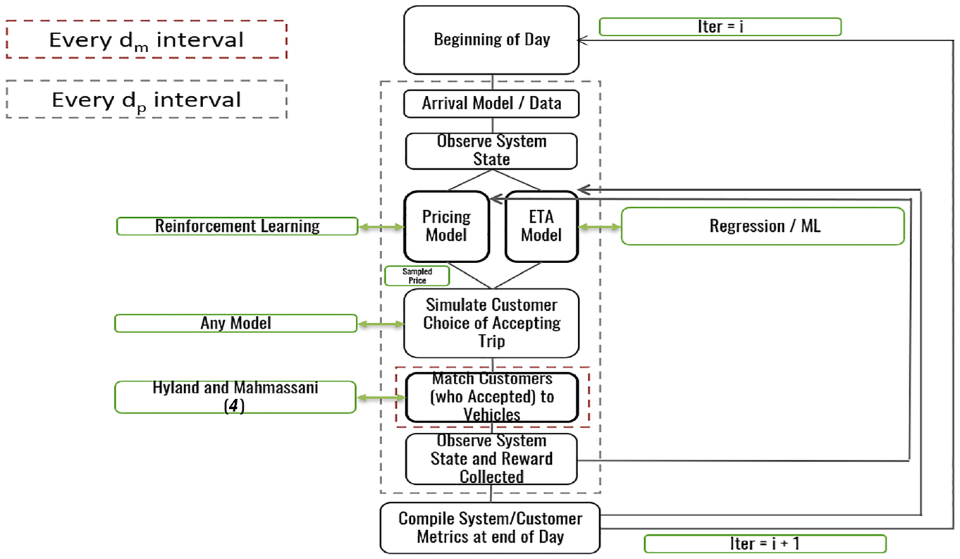
Simulation framework.
Simulation Results and Discussion
A randomly selected day of a taxi dataset in Chicago was used for simulation. The same dataset is repeated over different days (episodes) and convergence is checked afterwards. This dataset has information on the pickup and drop-off locations of trips as well as the request time of rides. There are 29,981 rides in the dataset to be served by 150 AVs with an average speed of 27.2 mph.
The spatial distribution of the trips is shown in Figure 3 (those with requested pickup times from 8 to 9 a.m.). Most of the trips are located near the Loop and along Lake Michigan with some trips originating from the suburbs and the airport (at the top left). Figure 4 shows the temporal distribution of requests. Dynamic pricing is performed every 5 min and matching of vehicles to customers is performed every 30 s.
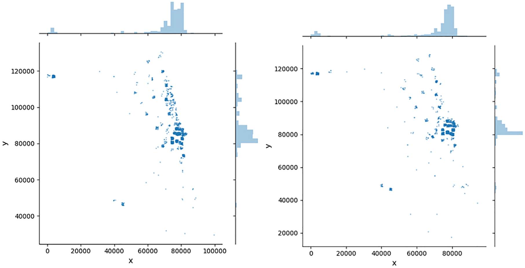
Spatial distribution (8–9 a.m.) of pickup locations (left) and drop-off locations (right).
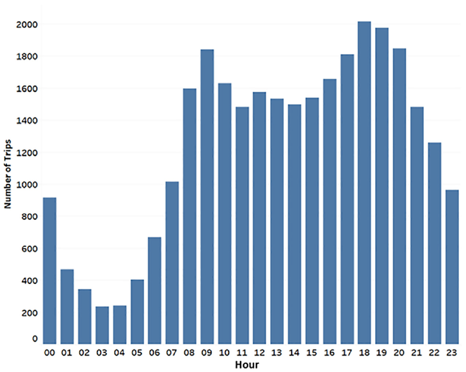
Temporal distribution of requests.
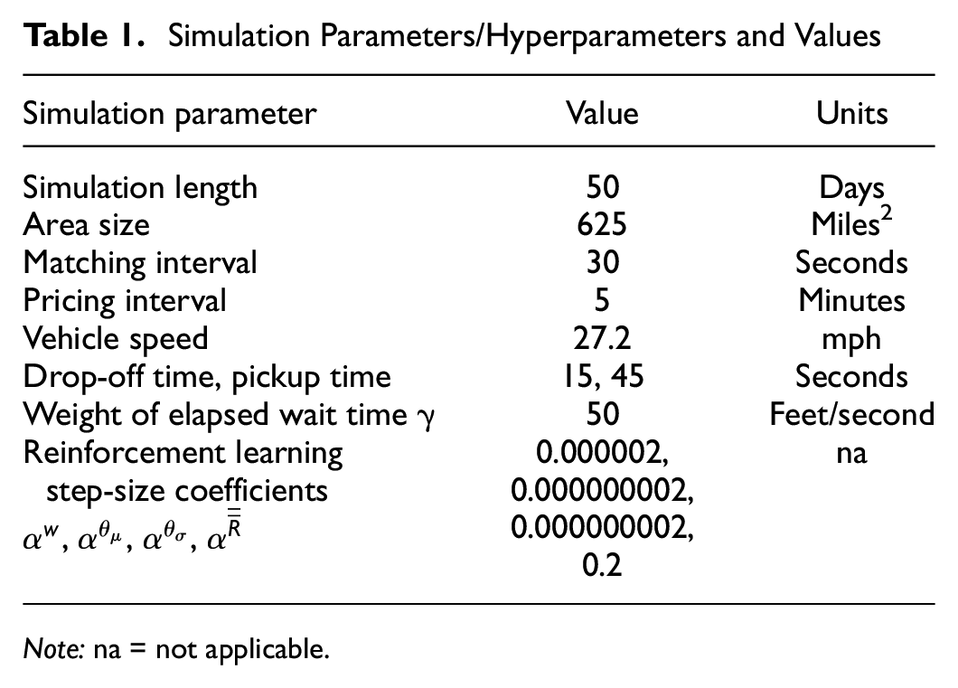
Table 1 lists the simulation parameters and hyperparameters used. Note that numerous hyperparameters of the RL algorithm were tested to find the most suitable ones. As a starting point, we used Sutton and Barto’s ( 5 ) rule of thumb for setting the parameter of linear stochastic gradient descent methods as follows. Assume you want to learn in τ experiences with a reasonably similar feature vector, then:

where x is a random feature vector (one can use an expected feature vector or check throughout the simulation). Moreover, we follow Sutton and Barto’s (
5
) recommendation whereby we use a greater step-size coefficient for the critic (
Simulation Parameters/Hyperparameters and Values
Note: na = not applicable.
The simulation was performed on a 24 Core Intel XEON CPU (3.0 GHz) machine with 128 GB RAM. Simulating 50 ridesharing days with the complete framework of Figure 2 took approximately 23 h. The simulation is coded in Python with the optimization problem solved with Gurobi 9.1.0., while linear regression is implemented with scikit-learn 1.1.0.
Figure 5 shows the learning process of the model’s pricing decisions. It takes near 20 days for the model to converge, reaching a maximum possible revenue of ∼$520,000. The figure shows the learnt means of the Gaussian parameterization of the surge multipliers (to show the patterns more clearly) over days 1 (Figure 5a), 5 (Figure 5b), 15 (Figure 5c), and 25 (Figure 5d). These are accompanied with specific metrics that we track: (1) revenue; (2) wait time (mean and standard deviation); (3) number of unassigned customers by the end of day (sanity check); (4) number of served customers at the end of the day; and (5) fleet utilization. Interestingly, we observe that the model learns by itself to price high when demand is high, and low when the demand is low, resembling the demand pattern shown in Figure 4. The plots also show the advantage of dynamic pricing over static pricing. Comparing days 5 and 25 (note that we are using day 5 as a reference as a conservative estimate that avoids arbitrary initial conditions), we see that revenue increases from $274,850 to $522,169 (90% increase) while wait time substantially decreases from 28 min to nearly 3 min (90% decrease), reaching an equilibrium that reflects the customers’ willingness to accept ride characteristics. Moreover, the number of unassigned customers at the end of the day reaches near zero at convergence, which serves as a sanity check that there are no huge wait time outliers, while the number of served customers stabilizes to fulfill near 72% of the demand.
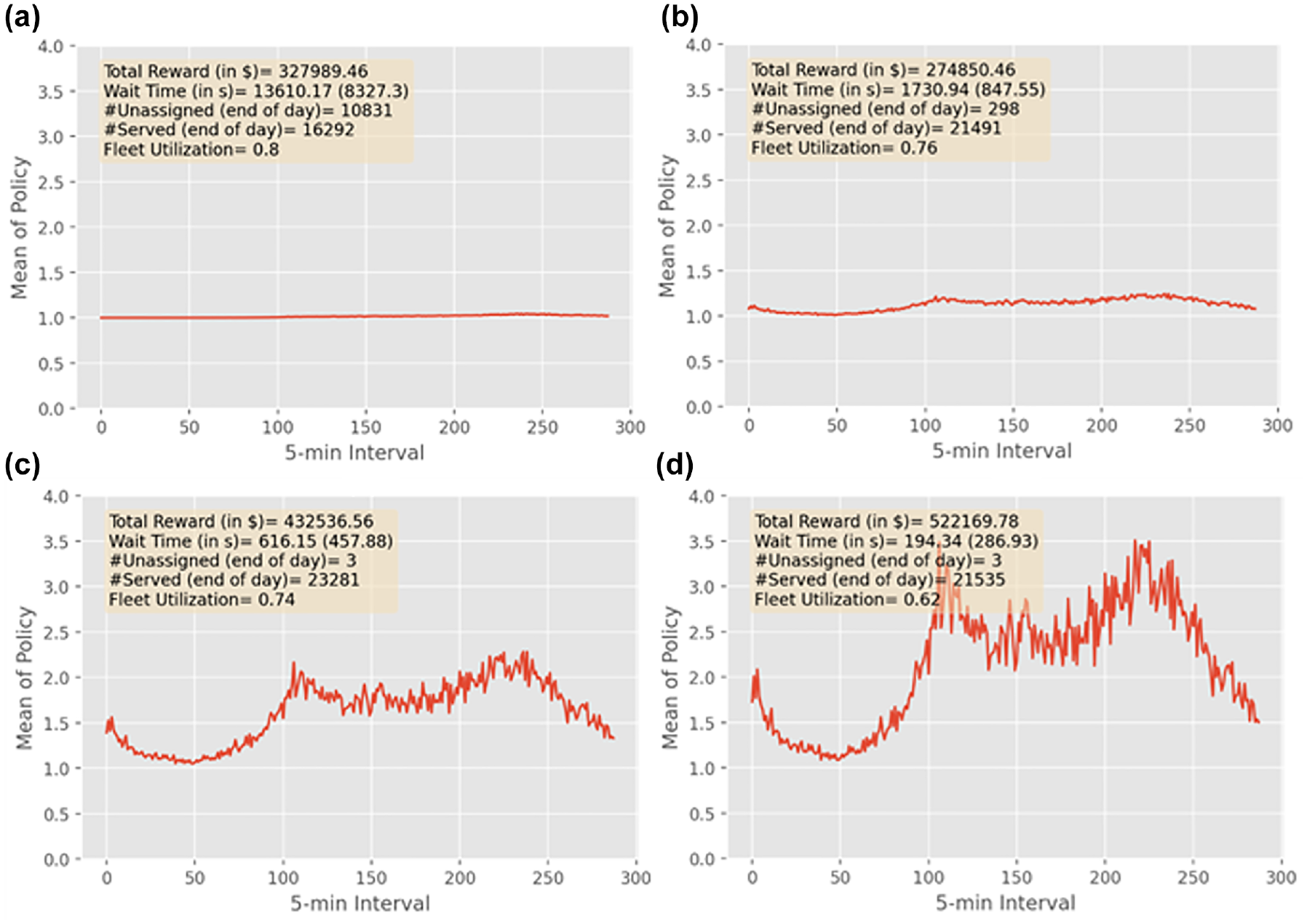
Mean of surge multiplier across days: days 1 (a), 5 (b), 15 (c), and 25 (d).
Scenario Testing
We develop two scenarios to test the robustness of the RL algorithm to detect nonstationary behavior, as follows.
Scenario 1
In this scenario, a sudden shock in the system occurs whereby the customers’ willingness to pay drastically changes (e.g., COVID-19). In our framework, we do this by changing the coefficient of price
Scenario 2
In this scenario, a slow change occurs to customers’ willingness to pay over time. In our framework, we do this by decreasing the coefficient of price
Figures 6 and 7 summarize the results. Note that on the first day, various initialization conditions for the RL algorithms and because the prediction models do not know how to estimate wait times well (yet) leads to the sudden drops in the figures. We see that the model takes nearly 20 days to converge. Scenario 1 shows that although the shock greatly decreased revenue on the 35th day, the algorithm was able to detect changes in the reward structure and adjust the algorithm’s parameters quickly. The robustness of the algorithm is not very clear in scenario 2 and therefore we run further simulations to compare the performance. The first is the full information case, that is, knowing the customers’ choice probabilities. Therefore, the reward in this is defined over all customers considering the choice probabilities, as follows:

where
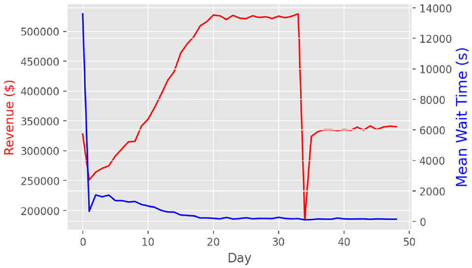
Scenario 1 revenue and wait time results.
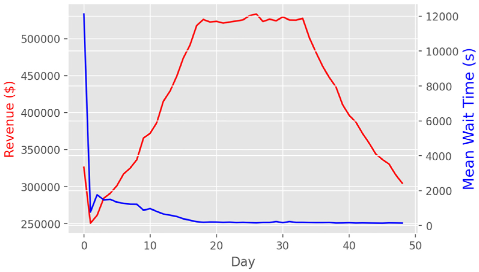
Scenario 2 revenue and wait time results.
The second case is using the converged RL model without any sampling of the surge multiplier after day 25 (i.e., no learning since the policy parameters do not get updated). This case also serves to show the power of sampling actions.
Figures 8 and 9 show the results. In scenario 1, the full information case performs the best as it provides accurate expected revenue even when the demand model’s parameters change; this results in updates of the RL’s parameters in the right direction and size. Nevertheless, our formulated version of the reward structure that does not rely on any information of the demand performs comparatively well. Finally, we see that RL pricing (both converged and full information case) can learn quickly (within one day) and increase revenue compared to what the converged model can achieve. These show that continuously sampling actions (i.e., continuous experimentation) can be a powerful tool and can increase robustness to system shocks. In scenario 2, the RL algorithm performs similarly to the full information case, with both of the algorithms showing superior performance over a converged modeling tactic. This further showcases the robustness of RL algorithms to optimize under changing environments.
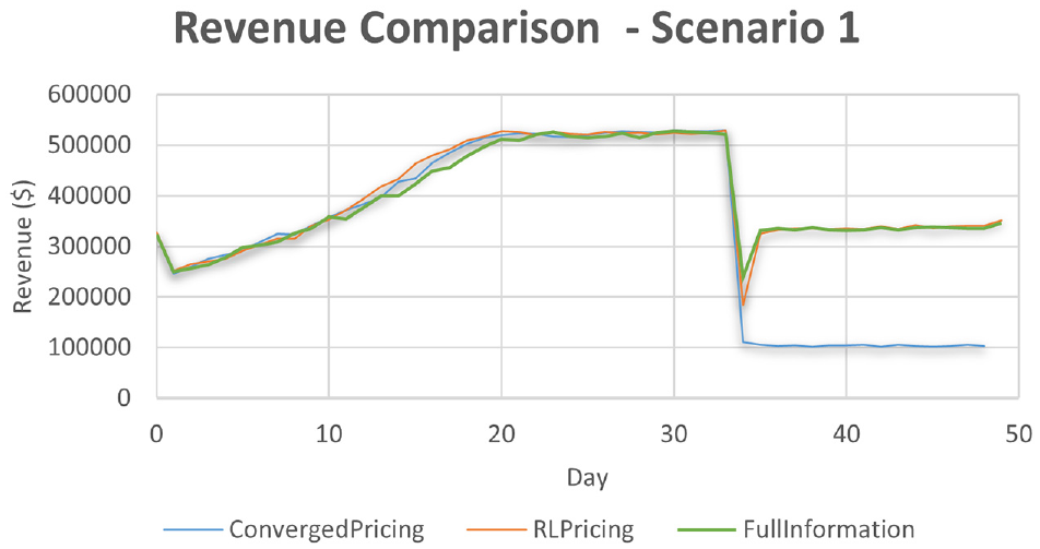
Comparison of reinforcement learning to converged pricing and full information cases in scenario 1.
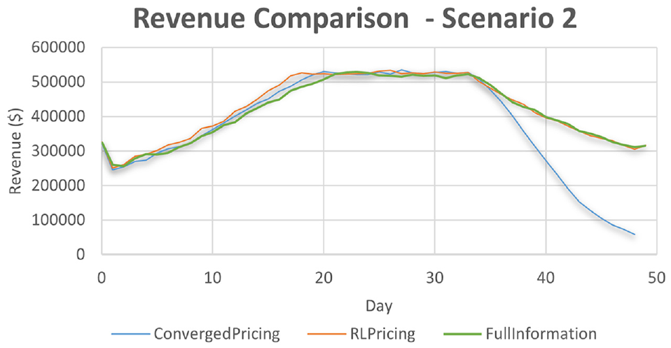
Comparison of reinforcement learning to converged pricing and full information cases in scenario 2.
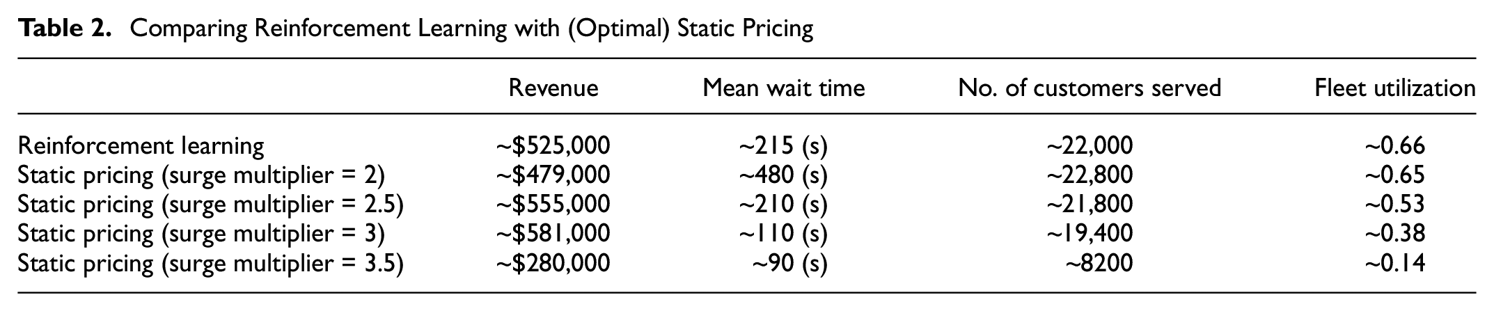
Finally, we use results of the RL model’s pricing decisions (Figure 5) to guide us in selecting multiple static pricing multipliers (i.e., the same surge multiplier across the day). Note that these surge multipliers are decided after-the-fact, that is, after receiving insights from the dynamic pricing surge multipliers. The results are shown in Table 2. Comparing to the (optimal) surge multiplier of 3, we see that RL can achieve near 90% of the revenue achieved by optimal static pricing, which is quite high. Nevertheless, RL was able to serve more customers with reasonable wait time. There are a few points to consider with respect to the above results. Firstly, the revenue result resembles that of Banerjee et al. ( 8 ) with respect to dynamic pricing not outperforming static pricing, but disagrees with most of the other literature. One difference to highlight is that this paper studies a fixed fleet system, which is likely to provide different insights because of the vehicles being always available. One also needs to note that RL attempts to optimize under an uncertain environment with no knowledge of the future. The static pricing surge multipliers were chosen using the guidance of the results from dynamic pricing, after knowing where to search. Specifically, since the static pricing methodology does not incorporate any online learning capability, RL’s value further increases when considering robustness. Further, note that the specific setup of the problem may affect results. For example, the customers’ choice model is the same across the entire day, which may not be entirely realistic. Finally, note that deep learning methods should be investigated in future work with such fixed fleets, either at the actor stage or the critic, since these methods may better capture nonlinearities in the system and provide higher revenue.
Comparing Reinforcement Learning with (Optimal) Static Pricing
Conclusion
This paper formulates a continuous pricing problem as a MDP and presents a simulation of SAMSs with algorithms to price rides, provide customer with wait time estimates, and match vehicles to customers. An average-reward RL formulation is presented to solve the MDP with a complex demand model that includes heterogeneous customers accepting the trip characteristics (price, expected wait time) probabilistically.
Insights from a fixed fleet operation of an autonomous private ridesourcing system in Chicago are presented. The converged model achieves an increase in revenue of 90% relative to day 5 of the simulation with a corresponding decrease of 90% in waiting time (note that we are using day 5 as a reference as a conservative estimate that avoids arbitrary initial conditions). However, after gathering insights of the RL algorithm, optimal static pricing (at a specific surge multiplier) shows that RL can achieve near 90% optimality in revenue with reasonable wait times offered to customers. Considering that RL attempts to optimize under an uncertain environment with no knowledge of the future, its performance is reliable and its value further increases when considering robustness. Two robustness scenarios are tested. In the first, a sudden shock occurs to the system whereby the coefficient of price changes drastically. In the second, customer’s willingness to pay changes slowly. In both scenarios, RL can quickly adapt its parameters to increase revenue, showcasing the robustness of the algorithm.
This work introduces several research aspects that can be addressed in future work. Firstly, a global pricing mechanism was employed in this paper, rather than an OD-based method. The latter may improve revenue, customer wait times, or both. Secondly, one day of data was used to learn across days/episodes; however, the question remains whether the algorithm can learn using different data across days, and if so, how to assess convergence. Future research can also study demand spikes (e.g., special events) and how these should be considered in training models, that is, should the model train on such outlier events or should it learn to adapt its parameters in real time? Fourthly, the customer wait time algorithm may be improved with machine learning techniques rather than linear regression. Fifthly, future research should take into consideration customer cancellation probabilities and how to correctly design algorithms to minimize cancellations resulting in system disturbances. Moreover, although this paper assumes fixed vehicle speed, the effect of congestion could readily be incorporated in optimizing such ridesourcing systems. Finally, this paper does not implement deep learning methods, which may better capture nonlinearities in the system. Other reward structures may also be studied to assess other aspects of the system (e.g., fairness, fleet utilization, etc.). A comparison of the continuous methodology with other RL-based algorithms should also be done in future work.
Footnotes
Author Contributions
The authors confirm contribution to the paper as follows: study conception and design: H. Abkarian, H. Mahmassani; data collection: H. Abkarian; analysis and interpretation of results: H. Abkarian, H. Mahmassani; draft manuscript preparation: H. Abkarian, H. Mahmassani. All authors reviewed the results and approved the final version of the manuscript.
Declaration of Conflicting Interests
The author(s) declared no potential conflicts of interest with respect to the research, authorship, and/or publication of this article.
Funding
The author(s) disclosed receipt of the following financial support for the research, authorship, and/or publication of this article: This research is funded through the Northwestern University Transportation Center’s Dissertation Year Fellowship.
The authors remain solely responsible for all contents of this paper