
Abstract
Municipalities make significant efforts with limited resources to collect pavement condition data. Overall Condition Index (OCI), which uses the pavement surface evaluation and rating manual to identify roadways needing repair, is a convenient and common way of pavement condition assessment. Many data used in assessing the OCI are collected from fieldwork. Some data features give little insight into road conditions, and one feature may provide similar information to another; thus, effective data-collection resources can be optimized by selecting which data feature to keep and which to discard. In addition, the OCI reflects how local agencies highlight the important variables driving their pavement-management investments. It is also a reflection of the triggers that they use to propose various treatment strategies. This research aimed to evaluate pavement distresses in West Des Moines, Iowa, using machine-learning methods, and determine which combination of distresses and their distress proportions can accurately predict the OCI class of a particular pavement type. The wrapper feature-selection methods were used, fitting their results to classification-tree models. Automatic feature selection, using Featurewiz, was also considered to select the desired number of variables. Feature parameters were screened for OCI prediction using the mean decrease impurity, and the results could be used to model classification that may be used for year-long predictions. Results showed that an effective OCI estimate methodology could be determined with significant accuracy with fewer features.
Keywords
Pavement performance and condition are crucial elements in the pavement-management system (PMS), where they determine maintenance and estimate the current and future resource allocations required (
1
). Evaluation of pavement performance and condition, including the estimation of friction, surface roughness, pavement structure, and existing distresses, plays a significant role in monitoring the overall serviceability, identifying maintenance and rehabilitation needs of pavements, and judiciously allocating resources to maintaining good roads, pavement design, and rehabilitation in PMS (
2
). These estimates of performance and condition that are functions of distress type, severity, and density are usually quantified and evaluated by different stress-based and roughness-based indices (
3
,
4
). Examples of such indices are the Pavement Serviceability Index (PSI), Pavement Serviceability Ratio (PSR), Pavement Condition Rating (PCR), Ride Number (RN), Profile Index (PI), International Roughness Index (IRI), Pavement Condition Index (PCI), and the Overall Condition Index (OCI). The OCI is a numerical indicator utilized by North American transportation agencies like the Iowa Department of Transportation (Iowa DOT) (
5
). The OCI uses the pavement surface evaluation and rating (PASER) manual to identify roadways needing repair (
1
). PASER is a rating criterion developed by the Transportation Information Center, University of Wisconsin–Madison (
6
), which utilizes a visual inspection of pavements, by trained observers, to identify the types of surface distresses that exist and which subjectively determines the levels of severity of the distresses (
7
). Based on the visual inspection, an estimate of an OCI value based on a scale of 1 to 10 is made, where
Performing model-dependent wrapper feature-selection analysis to select the most relevant distresses that describe the OCI without considering the age and year of remedial action. The intuition behind this is to utilize a cost-effective and available way of determining pavement conditions.
Building classification models that can predict OCI based on the feature-selection results.
Evaluating prediction results based on common measures, showing that reasonably high scores can be obtained.
Evaluating the selected feature importance in predicting the OCI. These importances were to be calculated using the mean decrease impurity (MDI), which counts the times a feature is used in splitting a tree node, divided by the number of samples it splits.
Literature Review
Representation of road conditions and roughness is essential for proper road maintenance to preserve or improve traffic safety and optimize the cost of maintenance. Various methodologies are now in practice to generate different pavement-performance models. Performance models can be categorized into deterministic, probabilistic, and stochastic models, which have been extensively used to relate the pavement condition to one or more factors leading pavements to deteriorate (
9
,
10
). Many previously published research papers discussed IRI and PCI prediction using several factors, including age, traffic, surface distresses, structural condition, environmental conditions, and road characteristics. The models could be as simple as the relationship between the performance index and the pavement’s age or could be more complicated, using two or more variables. Age was found to be one of the most important factors in predicting the performance index in different studies. However, age data are not always available because of a lack of archiving maintenance actions, especially for local roads managed by local agencies (
9
). As shown in Table 1, numerous articles adopted machine-learning techniques to predict performance indices using one or more of the earlier-mentioned predicting features. Some used age as a predicting feature accompanied by other factors, but without including the surface distresses and structural condition as part of the used predictors. Others included surface distresses in the combination of the predicting features. However, just a few depended only on the surface distresses to predict the performance index. Deterministic and probabilistic models have been predominantly used since the early stages of pavement-management systems, and they are still in use these days. In the late 1990s and early 2000s, the employment of statistical learning methods increased tremendously. Artificial intelligence, including machine learning, has a wide and rapidly increasing application in civil and infrastructure engineering. Various machine-learning algorithms have been used for general pavement-management applications, and pavement-performance modeling in particular (
11
). Many studies dealing with performance modeling using machine-learning techniques have been published in the past 10 years, and a greater part of them have used Long-Term Pavement Performance (LTPP) data (
12
). Machine-learning methods have been used to model pavement performance in different ways depending on the performance index chosen to be modeled against the available predicting features. Mostly, IRI has been the index of interest in the literature. Artificial neural network (ANN), inspired by how the brain works, has been the most widely applied algorithm to model the relationship between the dependent variable and the predicting features (
12
). ANNs have been used in predicting pavement conditions and in construction engineering (
13
,
14
), transportation (
13
), pavement engineering (
15
), structure (
16
), and environment (
14
). According to Table 1 and the review done by Damirchilo et al. (
12
), it is notable that age and non-distress variables have been more frequently used than the distress variables. Moreover, even in cases where distress variables were used, they were accompanied by age and non-distress features. Only in a few cases were distress variables used without considering any other types of variables to predict the performance index. As indicated in Table 1, in almost all cases, when the initial-condition index or age was present as predicting variables, it was given the highest weight of feature importance for the employed model. On the other hand, when distress variables only were used, cracking was rated as the most important distress feature to predict IRI for flexible pavements (
17
–
20
), except for the study by Nguyen et al. (
21
) which cited rutting. Generally, the testing
Literature Review
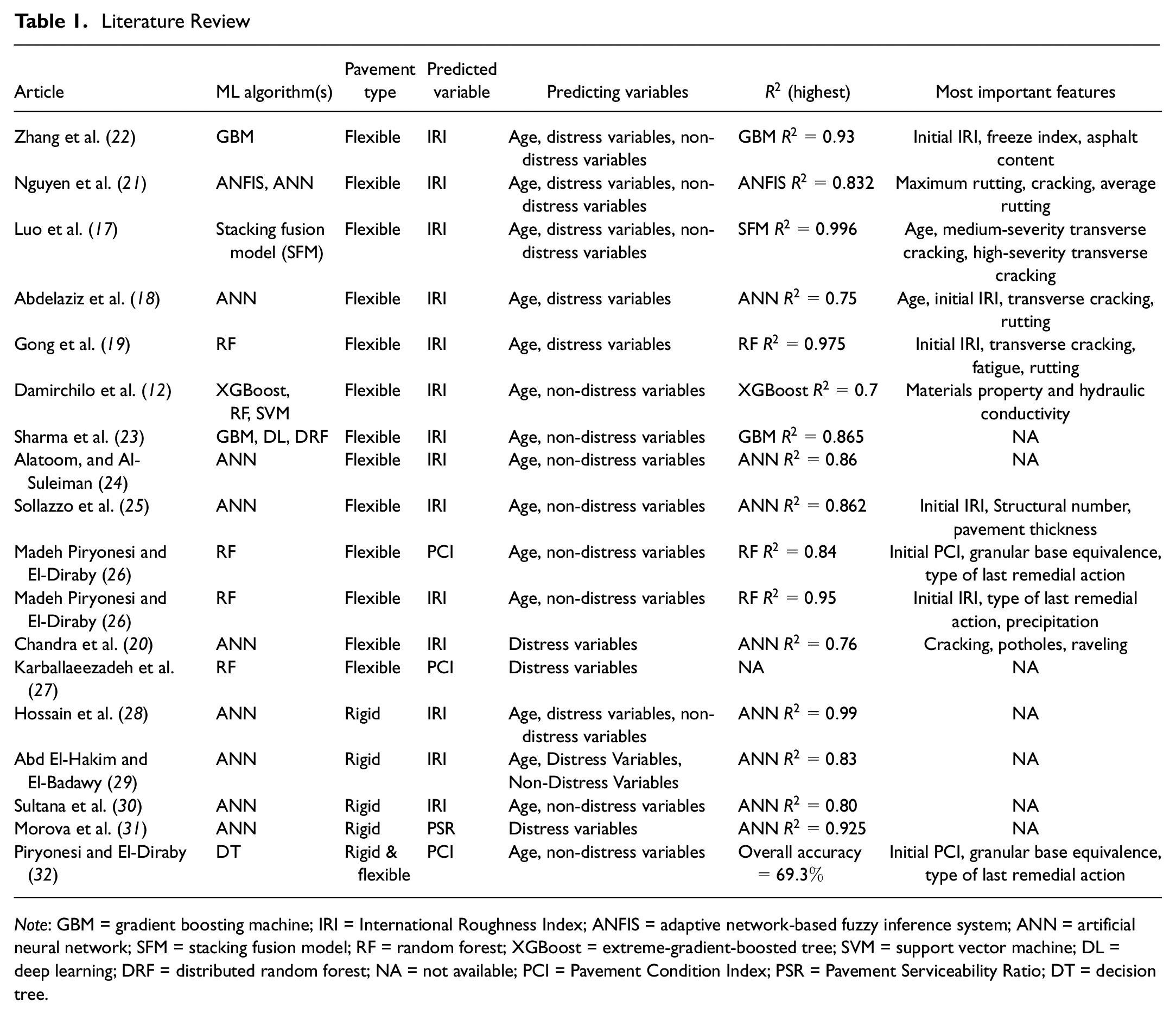
Note: GBM = gradient boosting machine; IRI = International Roughness Index; ANFIS = adaptive network-based fuzzy inference system; ANN = artificial neural network; SFM = stacking fusion model; RF = random forest; XGBoost = extreme-gradient-boosted tree; SVM = support vector machine; DL = deep learning; DRF = distributed random forest; NA = not available; PCI = Pavement Condition Index; PSR = Pavement Serviceability Ratio; DT = decision tree.
Feature extraction in modeling PCI and IRI was introduced in work such as that of Zeiada et al. ( 16 ) and Piryonesi and El-Diraby ( 33 ). In the latter, the initial PCI was developed from the distress values in the LTPP database. Then a set of pavement attributes was selected, mainly based on the ease of collection and cost-effectiveness. The researchers computed the feature importance in predicting PCI using seven statistical ranking algorithms and a feature-selection algorithm. Decision trees were trained based on asphalt roads and were developed to predict the future PCI deterioration level. The paper by Zeiada et al. ( 16 ) introduced the significance of pavement design factors for pavement performance in warm regions and compared them to a set of factors previously identified for cold regions. An ANN supported by a forward-sequential feature-selection algorithm was employed to identify the most significant design factors prevailing in warm climate regions using data extracted from the LTPP database. Researchers in Luo et al. ( 17 ) predicted IRI based on SFM and screened the feature parameters for IRI prediction using the MDI based on random forest (RF).
Data Preparation
For agencies to maintain roads in a good state, condition data need to be collected. Condition data are collected using either manual or automated data-collection methods. Before 2013, Iowa DOT funded data collection for local federal-aid-eligible (FAE) roads only, aiding local agencies in the state. However, starting in 2013, the state now collects distress data for all paved public roads every 2 years. The data collection in this research is fully automated by an Automated Road Analyzer (ARAN) van. The ARAN van collects and stores digitized video images of the pavement surface and processes them using pattern recognition with manual oversight to identify, quantify, and classify the types of distresses ( 34 ). Pavement distress is collected in one direction on two-lane highways or in two directions if there is a median. Data are collected for every 16 m section, identified by the street name, route name, county, city, latitude, and longitude using a differential global positioning system (DGPS). The OCI data in this research were collected over 3 years from 2013 to 2015 by the city of West Des Moines, Iowa. Each segment was given an OCI rating based on PASER ( 35 ). The OCI is based on a scale of 1 to 10. During evaluation and estimation, an immediate conclusion may be made to recommend a pavement repair or a time may be given before a repair is needed. The automatically collected data are spatially joined to the OCI data. All this information is used to update the street-segment data in geographic information system (GIS) format. More information is to be found in Bou-Saab et al. ( 1 ) and Bektas et al. ( 34 ). The total number of raw data records was 8321, of which 2172 were for composite-pavement data, 5941 for concrete, and the rest for other pavement types. After cleaning and preprocessing the data, composite-pavement data were reduced to 2006. For concrete pavement, average faulting values were not collected before the year 2015; therefore, many faulting data were missing. In the clean data, the number of records with faulting considered is 1725 and the number without faulting is 5218. Relevant distresses, and their meanings after preprocessing, are explained in Table 2. The notation 1 indicates that a feature was used in the overall prediction of an OCI and 0 indicates otherwise.
Explanation of Features
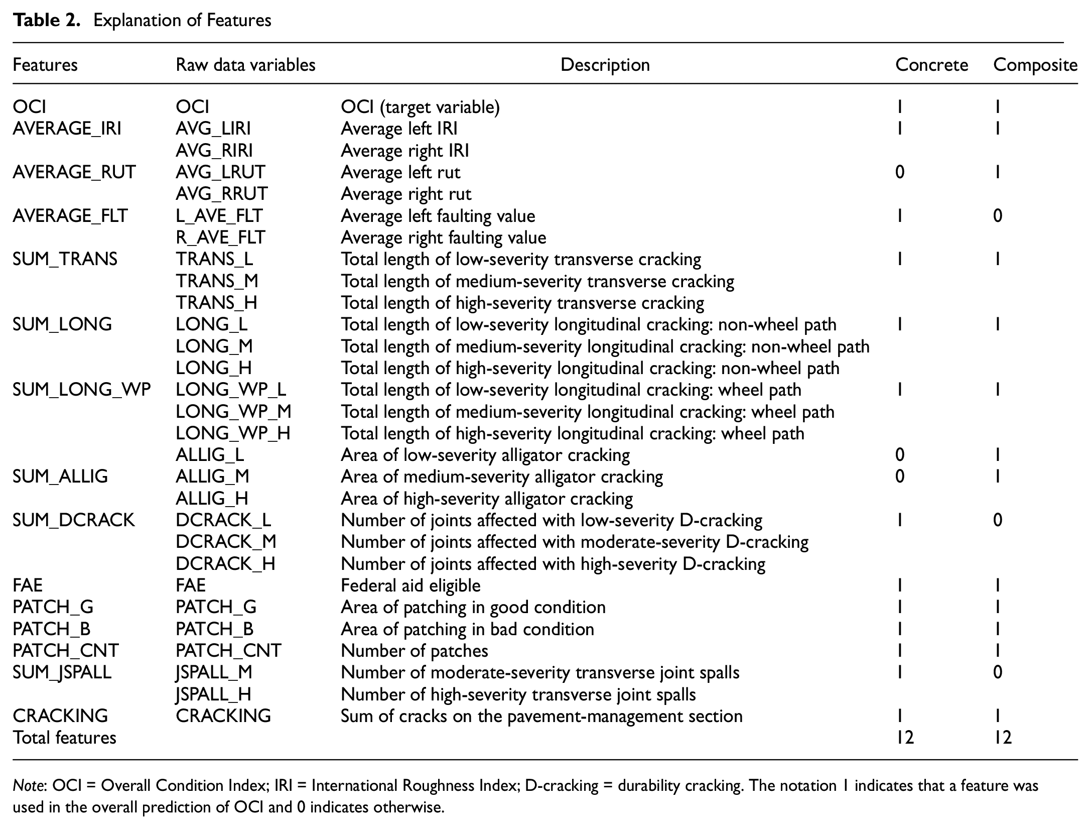
Note: OCI = Overall Condition Index; IRI = International Roughness Index; D-cracking = durability cracking. The notation
Methodology
The OCI assigned to each road segment by the city engineer through the PASER technique is categorized into five classes using an ordinal scale for evaluation purposes ( 1 ). The newly defined OCI scale, which ranges from 1 to 5, is utilized to describe the overall pavement condition, as shown in Table 3.
Categories of OCI into Different Levels
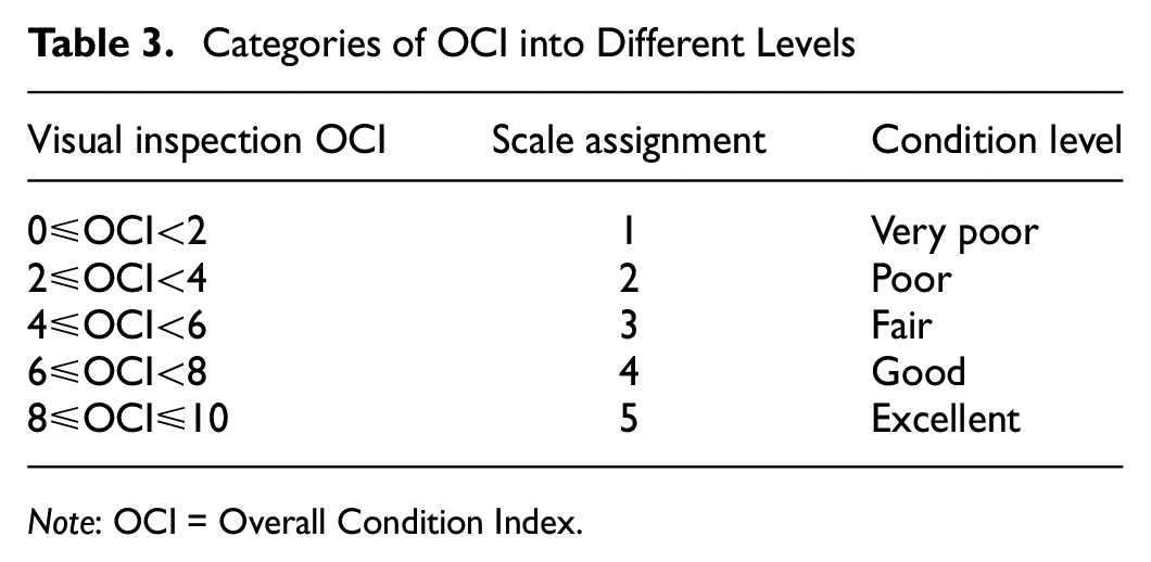
Note: OCI = Overall Condition Index.
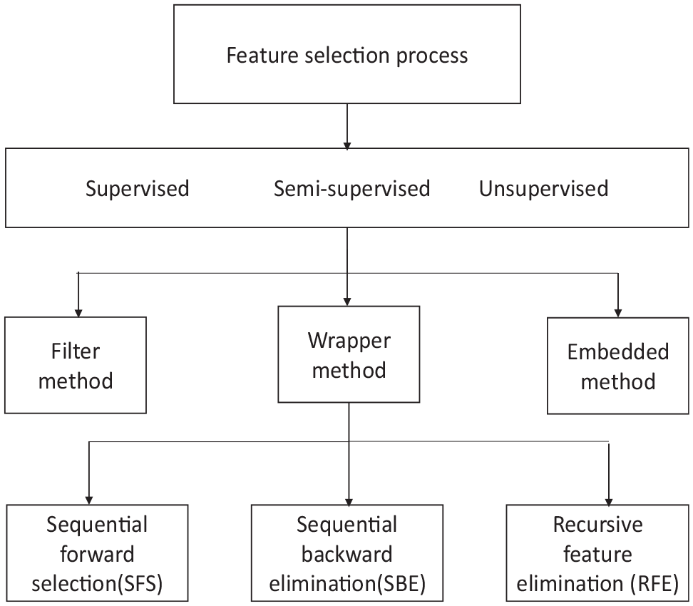
This paper focuses on feature selection and classification based on scale assignment. Models for each pavement type, concrete/rigid (PCC), and composite (COMP) pavements are developed with OCI as the target feature. The objective is to predict a municipal OCI using fewer features and excluding the age of the road and maintenance history. The rationale is that Iowa municipalities do not keep a complete maintenance record with the distress data and ages. First, data are collected, cleansed, and transformed, and each feature is normalized to its standard unit size. The normalized data are then passed on to the feature-selection algorithms: sequential forward selection (SFS), sequential backward elimination (SBE), recursive feature elimination (RFE), and Featurewiz. The first three methods are tuned to the models proposed: RF, gradient-boosted tree (GBT), and extreme-gradient-boosted tree (XGBoost). These designed models are evaluated, and the individual model-based feature importance is shown visually. Figure 1 describes the methodology of this research. Data are obtained, preprocessed, transformed, and then normalized. Normalized data are evaluated with various feature-selection methods and desired models. Selected features are then further subjected to training, testing, and cross-validation, where the scores and feature importance are then obtained.
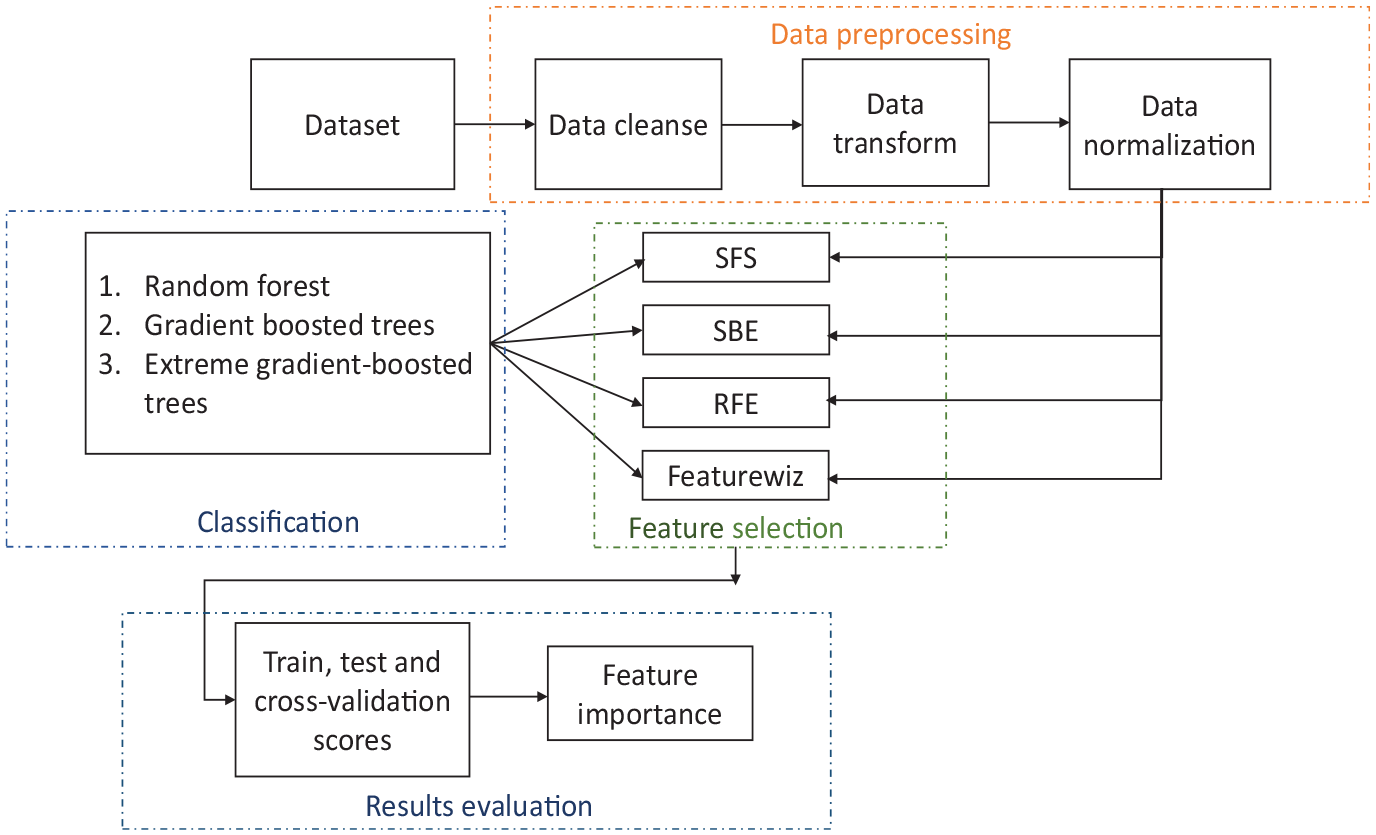
Proposed methodology.
Feature-Selection Methods
Feature selection reduces data dimensions by choosing a smaller subset from the original input variables (features) while eliminating redundant features and retaining the most relevant ones. The process may be tuned to a predictive model for a particular target feature ( 36 , 37 ). Some predictive modeling problems have many features that can reduce the efficiency of models and require large amounts of system memory space. Many models estimate parameters for every feature in the model. Because of this, the presence of non-informative features can increase the predictions’ uncertainty and reduce the model’s effectiveness. Reducing the number of features may lead to higher accuracy and better interpretability of models, and may improve the general performance of the model. Feature selection may be applied to supervised, semi-supervised, and unsupervised learning. The methods may be further classified as filter, wrapper, and embedded methods, as shown in Figure 2. Wrapper feature-selection methods require use of the intended machine-learning algorithm for prediction to evaluate the relevant features. Wrapper methods evaluate multiple models using procedures that add or remove predictors (features) to find the optimal features that maximize model performance ( 38 ). These methods are not automatic and require the specification of the quantity of desired features. The methods search the space of all possible subsets of features, measuring their effectiveness by learning and evaluating a classifier with that feature subset. The wrapper method of feature selection achieves better predictive accuracy than the filter method since the former is tuned to the specific interactions between the classifier and the dataset ( 39 , 40 ). It also overfits training data less than filter methods using cross-validation measures of predictive accuracy ( 41 ). Embedded methods are similar to wrapper methods in that they are computationally expensive and classifier dependent.
A tree of feature-selection processes.
Sequential Forward Selection
SFS is initiated with an empty selection of features. It starts with the best-performing feature against the target based on a set score. Then, newer features that maximize the model performance in combination with the previously selected feature are added one at a time ( 42 ). This procedure continues until the preset criterion is achieved ( 43 , 44 ). For each added attribute, the evaluation is estimated using cross-validation.
Sequential Backward Elimination
SBE works in the opposite direction to SFS. SBE initiates with the full set of features and, in each round, removes a remaining attribute of the given example set. For each feature removal cycle, the performance is estimated using the inner operators, such as cross-validation. The attribute giving the lowest performance score is removed from the selection. A new round starts with the modified selection and continues until the preset criterion is achieved. SBE can discard several features and allows for backtracking, so when a subset of features worsens the performance score obtained by the previous one, some previously eliminated features can be included in the new subset for re-evaluation. For each added attribute, the evaluation is estimated using cross-validation.
Recursive Feature Elimination
RFE recursively removes attributes and builds a model on the remaining attributes. It uses an accuracy metric to rank the features according to their importance. It takes the model and the number of required features as input and gives the ranking of all the features ( 45 ). Technically, RFE is a wrapper-style feature-selection algorithm that also uses filter-based feature selection internally in that it measures the relevance of features by their correlation with the target variable. RFE is different from SBE because while it targets individual feature coefficients, SBE tries to achieve the lowest score for the model as a whole. RFE selects features, given an estimator that assigns weights to features, by recursively selecting smaller sets of features. First, the estimator is trained on the initial set of features, and each feature significance is obtained. The least significant features are then cut from the current set of features. This procedure is recursively continued on the cut set until the preset criterion is met.
Automatic Feature Engineering Using Featurewiz
Featurewiz ( 46 ) is an automatic feature-engineering machine managed by the AutoViML lab. This method automatically preprocesses the data and then selects the best features by searching for the uncorrelated list of features (SULOV). SULOV finds pairs of highly correlated features. The correlation threshold is manually specified. After finding the pairs, their mutual information scores (MIS) are estimated, and the features with the least correlation and highest MIS are selected. The features selected from SULOV are recursively passed through an XGBoost algorithm, which then determines the best features based on the target feature. In this way, it selects the best features from the dataset. There is no need to specify the number of features or preprocess the data.
Machine-Learning Algorithm Models
Decision trees (DTs) have been used to predict pavement conditions. However, DTs have some drawbacks and are highly prone to overfitting. Ensemble learning methods like bagging and boosting have been created to improve the accuracies of DTs. Bagging builds several weak learners independently and combines them using some averaging methods. In boosting, the weak learners are built sequentially, and successive predictors are used to correct the errors generated by previous predictors to create a stronger predictive model ( 47 – 49 ). RF, GBT, and XGBoost are popular actualizations of ensemble learning of DTs.
Random Forest
RF is a bagging technique that combines several DTs on various subsets of the given dataset and takes their average to improve the accuracy of the prediction on that dataset. Instead of using only one decision tree, RF takes the prediction from each tree and finally outputs the result based on the majority votes of predictions. The greater the number of trees in the forest, the higher the accuracy and the lesser the problem of overfitting. RF error score converges to a certain limit as the number of trees in the RF increases. A forest’s error depends on the strength of the separate trees in the forest and their correlation. RF is more robust and less noisy than DTs. It gives useful internal estimates of error, strength, correlation, and variable importance ( 50 , 51 ).
GBT and XGBoost
In gradient boosting (
52
), the learning procedure consecutively fits new models to provide a better estimate of the response variable. The idea is to build new weak learners that are maximally correlated with the negative gradient of the whole ensemble’s loss function. Gradient boosting produces an ensemble of weak learners. When the weak learner is a DT, the algorithm is called GBT; it usually outperforms random forests. XGBoost (
53
) is a more regularized form of gradient boosting. XGBoost uses advanced regularization
Results Evaluation
Feature Importance
Feature importance shows the list of features the model considers the most relevant. It gives a score to each feature, describing the level of importance of that feature for the prediction of the target feature. It can be a score representing the features’ relevancy using an algorithm-based measure. MDI, the score utilized in this paper, counts the times a feature is used in splitting a tree node, divided by the number of samples it splits ( 17 ).
Evaluation Metrics Utilized
Given

In this paper, machine-learning algorithms have been applied to perform feature selection and prediction of OCI values. First, we collected data, preprocessed the data, and then applied different machine-learning algorithms to predict the OCI values. All data used were real-world data collected on real roads, and all experiments were coded on Jupyter Notebook Python 3.6. The models evaluated in this research are notated thus:
M1: Evaluation model: RF
M2: Evaluation model: GBT
M3: Evaluation model: XGBoost
M4: Feature-selection model: Featurewiz; Evaluation model: RF
M5: Feature-selection model: Featurewiz; Evaluation model: GBT
M6: Feature-selection model: Featurewiz; Evaluation model: XGBoost
M7: Feature-selection model: RFE; Evaluation model: RF
M8: Feature-selection model: RFE; Evaluation model: GBT
M9: Feature-selection model: RFE; Evaluation model: XGBoost
M10: Feature-selection model: SFS; Evaluation model: RF
M11: Feature-selection model: SFS; Evaluation model: GBT
M12: Feature-selection model: SFS; Evaluation model: XGBoost
M13: Feature-selection model: SBE; Evaluation model: RF
M14: Feature-selection model: SBE; Evaluation model: GBT
M15: Feature-selection model: SBE; Evaluation model: XGBoost
OCI Prediction/Classification for Composite Pavement
The composite-pavement data included 2006 clean data records. For all experiments, training, and testing data were obtained by a division of the data into 80% training and 20% testing. Cross-validation on the training data was done by further randomly splitting the training data 10 times. Results in Table 4 show how each model chose the features with its train, test, and cross-validation scores. A value of 1 indicates that the feature was selected, and an 0 indicates otherwise. The automatic feature-selection model, Featurewiz, was run first to determine the number of features for the other models. It was specified to be 10. In Table 4, out of the 12 features, AVERAGE_IRI, AVERAGE_RUT, SUM_TRANS, SUM_LONG_WP, PATCH_CNT, and FAE were features selected by all models. The accuracy scores show little difference between using all available data and reducing the features. This general observation of the result implies that we do not need all the features to predict the OCI. Figure 3 shows how each label distributed the feature importance. To obtain a high accuracy of the proposed models, SUM_TRANS, AVERAGE_RUT, and AVERAGE_IRI are the three most important features, based on their ranks. In this result, M13, the SBE with the RF model, offers the best model for the composite-pavement OCI prediction.
Table of Results for Composite Concrete
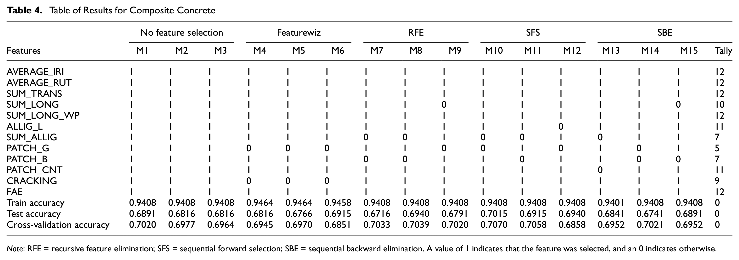
Note: RFE = recursive feature elimination; SFS = sequential forward selection; SBE = sequential backward elimination. A value of 1 indicates that the feature was selected, and an 0 indicates otherwise.
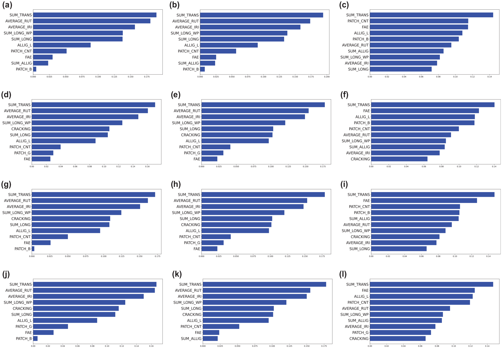
Feature importance of models after feature selection: (a) M4, (b) M5, (c) M6, (d) M7, (e) M8, (f) M9, (g) M10, (h) M11, (i) M12, (j) M13, (k) M14, and (l) M15.
OCI Prediction/Classification for Concrete Pavement with Average Faulting
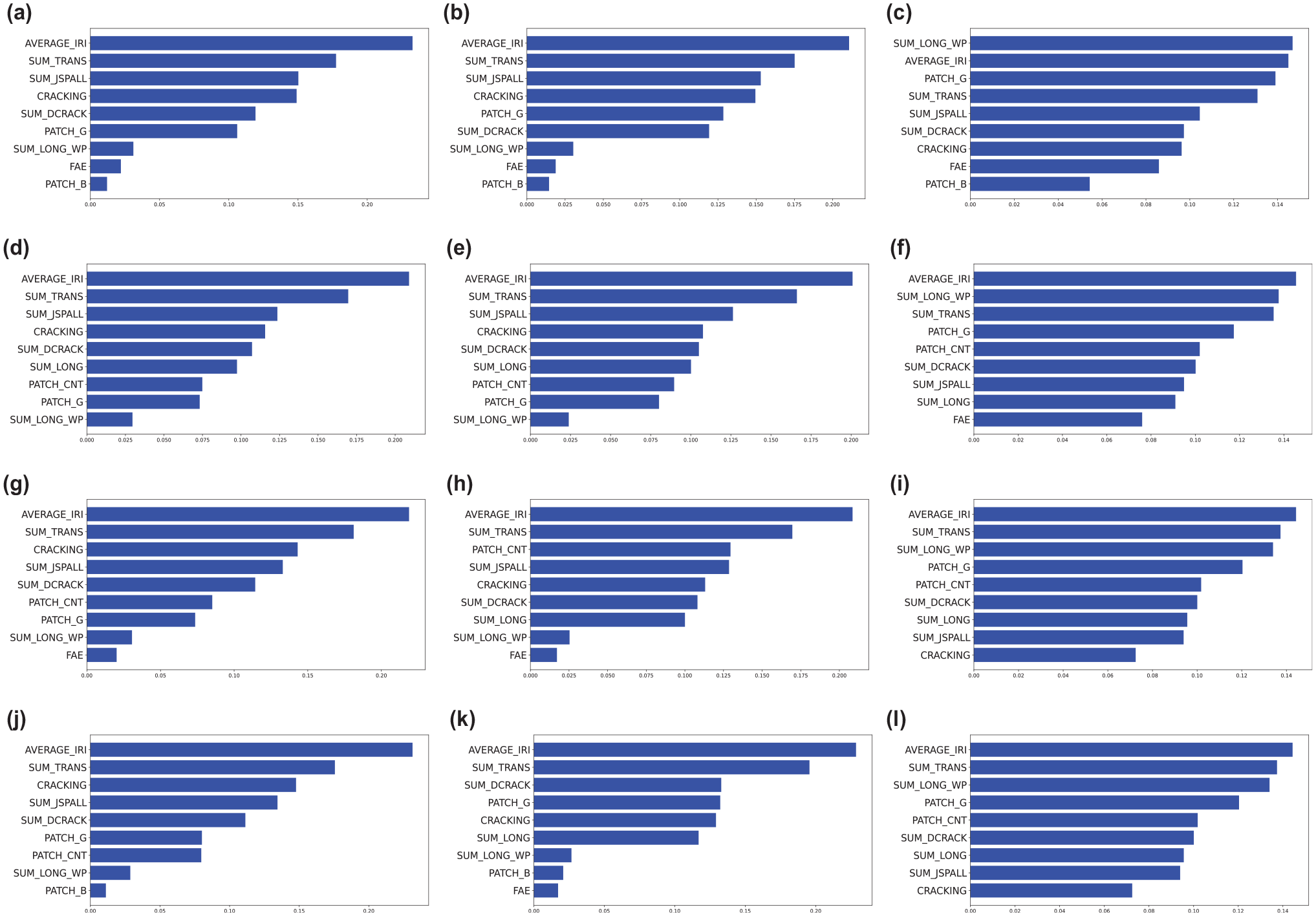
As previously mentioned, average faulting values were not collected before the year 2015; therefore, many faulting data were missing for concrete pavement. The number of data records with faulting considered was 1725. As above, the experiment divided training and testing data in an 80:20 split. Cross-validation on the training data was done by further randomly splitting the training data 10 times. Results in Table 5 show how each model chose the features with its train, test, and cross-validation scores. A value of 1 indicates that the feature was selected, and an 0 indicates otherwise. The automatic feature-selection model, Featurewiz, was run first to determine the number of features for the other models. That was also determined to be 10. In Table 5, out of the 12 features, AVERAGE_IRI, AVERAGE_FLT, SUM_TRANS, and SUM_LONG_WP were features selected by all models. The accuracy scores show little difference between using all available data and reducing the features. This general observation of the result also implies that we do not need all the features to predict the OCI. Figure 4 shows how each label distributed the feature importance. SUM_TRANS and AVERAGE_IRI are the two most important features, based on their ranks, for obtaining a high accuracy of the proposed models. SUM_DCRACK and SUM_JSPALL each seem to interchange their importance based on the model. From the figure, AVERAGE_FLT is not among the top five important features; therefore, it is possible to predict the OCI without the average faulting feature. Analytically, M4, Featurewiz with the RF, is the suggested model for this concrete-pavement OCI prediction.
Table of Results for Concrete Pavement with Average Faulting
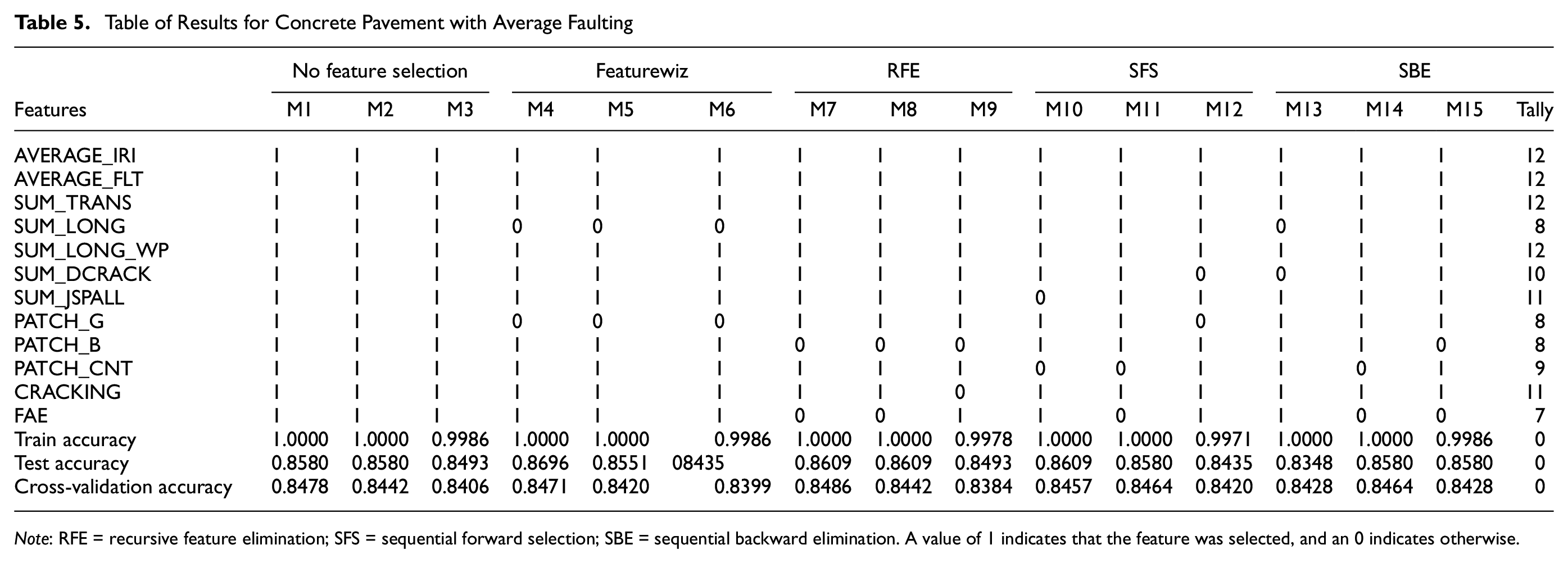
Note: RFE = recursive feature elimination; SFS = sequential forward selection; SBE = sequential backward elimination. A value of 1 indicates that the feature was selected, and an 0 indicates otherwise.
Feature importance of models after feature selection: (a) M4, (b) M5, (c) M6, (d) M7, (e) M8, (f) M9, (g) M10, (h) M11, (i) M12, (j) M13, (k) M14, and (l) M15.
OCI Prediction/Classification for Concrete Pavement without Average Faulting
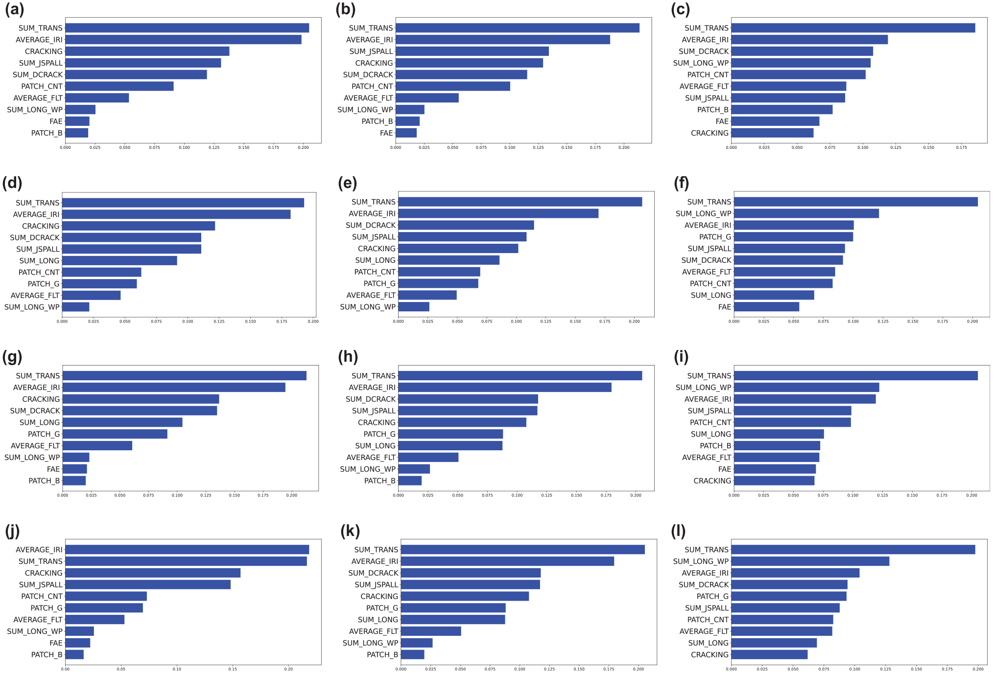
For concrete pavement without average faulting data, there were 5218 clean data records. Again, the experiment divided training and testing data with an 80:20 split. Cross-validation on the training data was done by further randomly splitting the training data 10 times. Results in Table 6 show how each model chose the features with its train, test, and cross-validation scores. A value of 1 indicates that the feature was selected, and an 0 indicates otherwise. The automatic feature-selection model, Featurewiz, was run first to determine the number of features for the other models. It was determined to be 9. From the accuracy results of 6 to 5, the training accuracy reduced by around 3%, while the test and cross-validation accuracies increased by around 3% to 5%. These increasing test/cross-validation results could result from the larger number of records of training data and the reduced training accuracy resulting from the average faulting feature. Either way, the results without faulting seem to achieve more predictive accuracy and thus are preferred. In Table 6, out of the 11 features, AVERAGE_IRI, SUM_TRANS, SUM_DCRACK, and SUM_LONG_WP were features selected by all models. Figure 5 shows how each label distributed the feature importance. AVERAGE_IRI and SUM_TRANS are the two most important features, based on their ranks, for obtaining a high accuracy of the proposed models. Analytically, M5, Featurewiz with XGBoost is the suggested model for this concrete-pavement OCI prediction. A good model can be obtained without faulting.
Table of Results for Concrete Pavement without Average Faulting
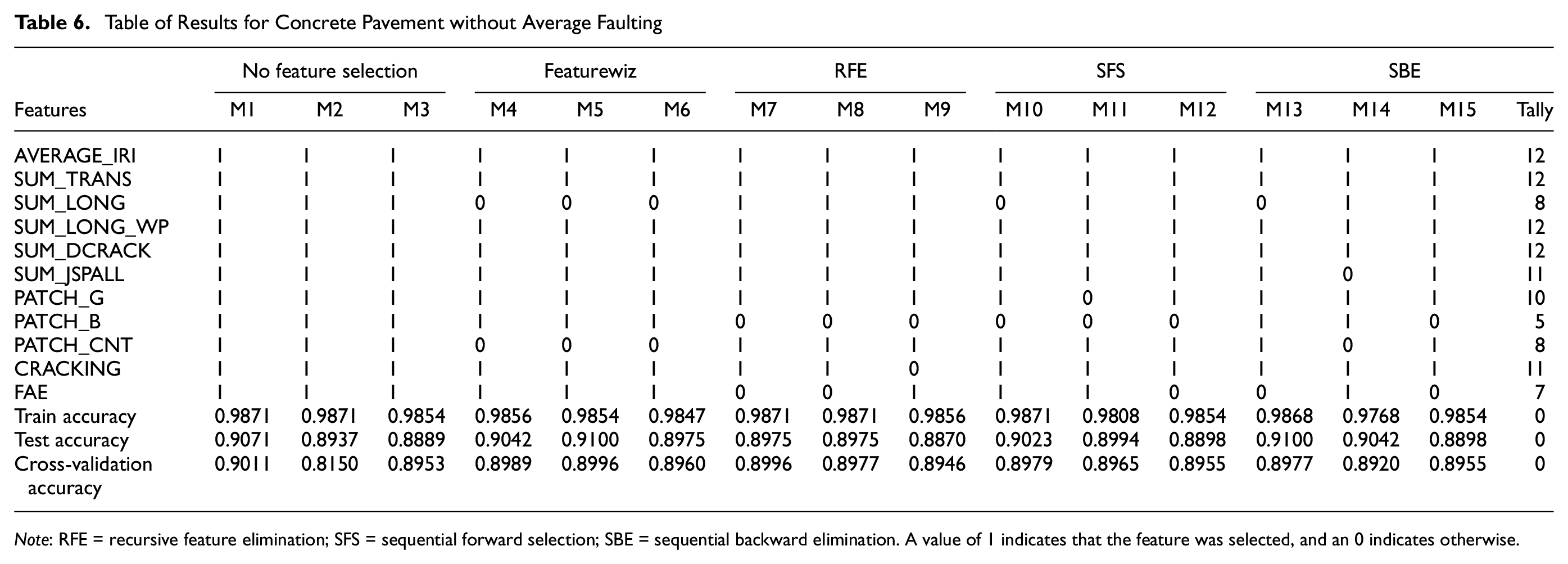
Note: RFE = recursive feature elimination; SFS = sequential forward selection; SBE = sequential backward elimination. A value of 1 indicates that the feature was selected, and an 0 indicates otherwise.
Feature importance of models after feature selection: (a) M4, (b) M5, (c) M6, (d) M7, (e) M8, (f) M9, (g) M10, (h) M11, (i) M12, (j) M13, (k) M14, and (l) M15.
Conclusions
This research evaluated pavement distresses in West Des Moines, Iowa, using machine-learning methods to determine which combination of distresses and their distress proportions could accurately predict the OCI class of a particular pavement type. The wrapper feature-selection methods (forward, backward, and recursive) were used, fitting their results to classification models (RF, GBT, and XGBoost). Automatic feature selection (Featurewiz) by combining searching for uncorrelated variables (SULOV) and XGBoost was used to automatically select the number of features. Numerical accuracies show that the model accuracies are maintained or increased with fewer features considered. Feature parameters were screened for OCI prediction using MDI.
Results indicate that other pavement condition indices might also be estimated with significant accuracy, with fewer features, and without age and maintenance histories, using a methodology similar to the one laid out in this paper. This estimation is especially useful as a data-driven approach to feature selection and estimating weights for each feature for accurately estimating the PCI. Depending on the outcomes of this research and the previously published research articles, the conclusions can be drawn that machine learning is not only beneficial for performance modeling but can also be used to update the PCI calculation procedure and to select the distresses that significantly affect the PCI value in such a way that the PCI value reflects the pavement condition more precisely. Based on feature importance, the agency can pick what distress data to collect or to devote to PCI calculation, as well as the appropriate weight to be given for each distress, based on its importance in representing the road condition as a PCI value. Another advantage of utilizing the proposed approach is overcoming the risk of missing age or initial-condition information impeding the forecasting process. This success was achieved by obtaining performance models that do not utilize age or non-distress variables as condition predictors. These feature-selection models can also be effectively applied to other pavement condition indices with available data.
Footnotes
Author Contributions
The authors confirm contribution to the paper as follows: study conception and design: Nlenanya, Adesunkanmi, Al-Hamdan; data collection: Nlenanya; analysis and interpretation of results: Adesunkanmi, Nlenanya, Al-Hamdan; draft manuscript preparation: Adesunkanmi, Al-Hamdan, Nlenanya. All authors reviewed the results and approved the final version of the manuscript.
Declaration of Conflicting Interests
The author(s) declared no potential conflicts of interest with respect to the research, authorship, and/or publication of this article.
Funding
The author(s) received no financial support for the research, authorship, and/or publication of this article.