Deep Learning Based Method for Early Warning of Price Risk in Railroad Bulk Freight Transport with Consideration of Time Series of Comprehensive Impact Index

Abstract

The aim in this study is to enhance the price competitiveness of medium- and long-haul railroad bulk cargoes in the transportation market. Efficiently triggering an early warning for railroad bulk freight price risk is crucial. This paper discusses relevant factors affecting the pricing of railway freight from four aspects, namely the macroeconomy, the transportation market, the freight owner, and the railway enterprise. We construct a comprehensive index system for generating an early warning of railroad bulk freight prices. Utilizing a collected data set of 20 factor indicators that affected prices from 2015 to 2017, we calculate a comprehensive price risk warning index using the integrated entropy weight and the Technique for Order Preference by Similarity to Ideal Solution (TOPSIS) method. We propose a risk warning level classification method based on the k-means clustering method to determine five levels of price risk warning. Subsequently, we establish comprehensive index prediction methods for issuing price risk warnings based on the back propagation (BP) neural network and the deep learning long short-term memory (LSTM) network. We verify that the prediction performance of the deep learning LSTM network is significantly better than that of the BP neural network by combining all coal freight data from the Shanghai Railway Bureau for the period 2015 to 2017 as a case study. The proposed method can predict the level of freight price risk more accurately in the next phase, based on the status of the factor indicators, and be used to assist railway departments in developing a more reasonable freight price adjustment strategy to scientifically mitigate freight price risk.

Keywords

railway bulk freight price risk warning BP neural network LSTM neural network deep learning

China’s railways transport overall higher volumes of goods at lower costs and with fewer operational risks, compared with other transport modes. Rail is the main mode of transport for bulk cargo in China and has a very important position in the transport market. The setting of railway freight prices will have a significant effect on the national economy. The government has regulated the setting of railway tariffs for a long time. In recent years, with the development of the market economy and the increasing demand for a green, low-carbon economy and environmental protection, the railway sector is also vigorously promoting the construction of road-to-rail projects and constructing dedicated railway lines for large industrial and mining enterprises, logistics parks, and ports. However, other modes of transportation continue to compete for market share in the transport industry. For example, from January to September 2021, Inner Mongolia’s coal production was 833 million tons, and road transport of coal was 394 million tons, accounting for about 47% of all coal transportation. Compared with 2020, the year-on-year growth rates of rail and road freight volumes are about 20% and 22%, respectively, indicating that road transport is growing faster than rail transport. This threatens the market position of railway transportation.

In the actual operations of railway transportation enterprises, there are still issues concerning poor control of the balance between transport volume and pricing in the formulation and management of transportation prices. In the transportation of bulk cargoes especially, the highest percentage of freight is coal cargo transportation. Coal supply enterprises tend to determine transport prices and transport volumes by signing medium- and long-term agreement contracts with railway companies. For example, the coal freight target set by China Hohehot Railway Bureau for 2022 is to transport 242 million tons, with 130 million tons (54%) allocated to coal shipments through medium- and long-term contracts. In transporting the remaining 46%, it is necessary to rely on rail spot contracts to fulfill coal transport targets, leading to competition with road transport for freight market share. Moreover, the medium- and long-term contract performance rates do not generally exceed 90%, that is, at least 10% of medium- and long-term contracts cannot be fulfilled as agreed. Consequently, in the railway sector, it is still necessary to make an effort to compete in the coal transportation market through pricing strategies and improvements in transport service quality. A key aspect of this work involves actively securing additional spot transportation contracts. When the market fluctuates, the prices of medium- and long-term contracts are constrained by the terms of the contracts, which cannot be readily adapted to match changing market conditions. In contrast, the pricing framework for coal spot transportation contracts offers a relatively high degree of flexibility. During periods of elevated coal prices, there is a surge in market demand for coal transport. The high costs associated with road-based coal transportation prompt a shift toward the more economical railway transport option, consequently resulting in a shortage of railway transport capacity. Conversely, when coal prices are low, the market demand for coal transportation diminishes. This, in turn, leads to coal supply enterprises to greatly reduce the performance rate of railway medium- and long-term agreement transportation contracts, resulting in a waste of railway transportation capacity.

In January 2015, Chinese Government departments issued a notice on the adjustment of railway freight prices to further improve the price formation mechanism; this increased the national uniform freight tariff for railway freight from an average of RMB 0.1451/ton-km to RMB 0.51/ton-km. On this basis, a certain degree of fluctuation in tariffs is permitted, allowing for an upward fluctuation of no more than 10% and an unlimited downward fluctuation. This provides railway transport enterprises with a certain degree of autonomy in pricing. Subsequently, in 2018, the authorities implemented government-guided pricing for the transportation of full rail carloads of goods. This pricing structure incorporates flexibility based on the original benchmark price. However, the pricing must comply with the requirements of the price fluctuation range. The rate of increase is adjusted from no more than 10% to 15%, with an unlimited range of downward fluctuation. In contrast, the market for road freight transport allows for free pricing. Therefore, we mainly compare the consideration of market risk for rail freight transport prices with the road freight transport market.

Furthermore, although there is a strong competitive advantage over road freight transport for short distances, when transporting freight over medium and long distances, between 800 km and 1,500 km, the level of competition becomes comparable to that of rail freight transport. In 2021, the average distance traveled by rail order for coal in China was 1,204 km. Thus, it is within this medium- to long-distance range of transport that the competition between road and rail freight is most intense. Price competition is the main form of transport mode competition.

The government generally coordinates the railroad bulk cargo business in China. Railroad carriers sign bulk cargo transportation agreement contracts with cargo owners in advance; these are options contracts. This approach effectively reduces the risk of revenue loss for carriers, owing to drastic price fluctuations in the railroad bulk cargo transportation market. However, China’s railroad bulk cargo transportation market coexists with the options and the spot market, so the price risk in the bulk cargo transportation market still exists. On the one hand, if the freight spot market price is low, it is difficult for railroad enterprises to obtain freight orders in the freight spot market without timely price decreases. On the other hand, lower freight prices in the railroad spot market will affect the performance of the cargo owners’ transport contracts. This is because spot market freight prices often fall considerably below the original contract prices, surpassing the losses caused by contract breaches. Cargo owners will abandon the execution of the original transport contract and instead turn to the spot market to buy capacity, so that the performance rate of the original signed freight contract will be greatly decreased. Railroad transport enterprises will bear the loss of revenue from the reduction of transport orders and waste of transport capacity. If the market price in the freight spot market is high, there are two aspects to consider. Firstly, existing railway transportation orders must still be fulfilled according to the contract terms, even with reduced profit margins. Secondly, owing to the lower prices offered by the railway companies, a significant number of freight orders originally intended for road transportation might shift to railways. As a result, railway carriers must ensure the fulfillment of these transportation contracts, which might initially yield low profits. Simultaneously, they face increased pressure to meet the surging demand for their transportation services. However, the remaining capacity resources might fall short of fully accommodating the demand for cargo transportation at relatively high spot market freight rates for capacity, leading to a missed opportunity to generate additional revenue.

The price risk in bulk cargo transportation is caused by too-high and too-low transportation prices in the spot market for capacity. This can result in profit loss and reduced revenue for carriers. Anticipating the presence of price risk assists carriers in effectively avoiding and mitigating such risks. Therefore, the accurate prediction and judgment of freight price risks, so as to issue price risk warnings, pose challenges and issues for railroad carriers.

The rest of this paper is organized as follows. The second section is a literature review. The third section establishes an indicator system for the early warning of price risk in railway bulk cargo transportation. In this section, a comprehensive early warning index of price risk is calculated by integrating the entropy weight method and the Technique for Order Preference by Similarity to Ideal Solution (TOPSIS) method. Furthermore, the k-means clustering method is employed to determine the early warning level for the comprehensive early warning index. In the fourth section, a freight price risk prediction method is constructed, along with performance evaluation metrics. These are based on the optimal deep learning long short-term memory (LSTM) parameter configuration and the BP parameter configuration. In the fifth section, a case study is presented, using the deep learning LSTM method with optimal parameter configuration for predicting the price risk of railroad bulk cargo transportation. This section also includes a comparison of the prediction effects with the back propagation (BP) neural network method. The last section summarizes these studies and presents the outlook.

Literature Review

Over recent decades, extensive attention has been given by researchers to the study of risk warnings in various sectors, including bank credit, corporate financial management, urban disasters, security warnings, hazardous materials warnings, and finance, shipping, and railroad transport.

Most studies in the field of bank credit use factor analysis ( 1 , 2 ), Fisher discriminant analysis ( 3 , 4 ), adaptive radial basis function algorithms ( 5 ), or multilayer perceptron neural network algorithms ( 6 , 7 ). In the field of corporate financial management, the most used risk early warning modeling methods are logistic regression prediction models ( 8 ), Cox regression models ( 9 , 10 ), and BP neural network algorithms ( 11 ). The main research methods for risk early warning in the financial sector include support vector machine (SVM) algorithms ( 12 ), Bayesian classification ( 13 ), Kaminsky–Lizondo–Reinhart (KLR) signal analysis ( 14 , 15 ), and LSTM neural network algorithms ( 16 , 17 ).

In relation to early warning research in relevant transport sectors, the main focus is on the shipping and railroad transport sectors. Yang et al. ( 18 ) developed an SVM-based freight rate warning model for analyzing and predicting freight rate volatility alerts in the shipping market. Based on the knowledge and experience of shipping experts and other relevant criteria, the actual freight rate warning levels in the sample interval of the shipping market were determined. Chen et al. ( 19 ) developed an early warning system (EWS) for predicting shipping market crises based on economic cycle theory and extended it by constructing a “climate index” analysis. Yun et al. ( 20 ) used a crisis signaling approach based on the Baltic dry index (BDI) and various other indexes, such as finance, economy, and shipping indexes, to create an EWS for the maritime industry. Choi et al. ( 21 ) developed an early warning index considering 60 independent variables, including shipping, shipbuilding, and finance indexes, and used mean square error and time lag correlations to verify its accuracy. In the field of railway transportation, Haji-Kazemi et al. ( 22 ) conducted a case study of a Norwegian high-speed rail project to analyze the early warning signs that might be found during the front-end phase of such a project and illustrate how these early warning signs can help in making major decisions, such as the level of feasibility and achievability of the project’s goals. For other fields of transportation, Gao et al. ( 23 ) analyzed the intrinsic relationship between the comprehensive transport volume index and gross domestic product (GDP) to identify extremely hot or cold problems in the development of the transport industry at an early stage and provide a basis for a risk warning system for the transport industry.

So far, there has not been much research on the price risks of railroad transportation or on creating early warnings of these risks. In this paper, we aim to fill this gap by constructing a price risk early warning method for cargo transportation covering distances ranging from 800 km to 1500 km, utilizing the deep learning LSTM neural network method. The method is based on the establishment of a price risk identification index system for railroad bulk cargo transportation in China. The index system takes into account four important influencing factors that affect cargo transportation prices. The proposed method facilitates more accurate prediction and judgment of the price trends of bulk cargo freight and provides early warnings of the risk associated with excessively high or low prices in medium- and long-distance coal railroad transportation. We have implemented a system for generating early risk warnings for railroad cargo transportation pricing, designed to assess the level of risk associated with such pricing. For railroad departments, this system guides the formulation of future transportation price policy based on the specific allowable price fluctuation range mandated by the government. It also serves as a reference for railroad departments, for establishing reasonable transportation prices within the permissible price range. Additionally, it aids in developing corresponding operational scheduling plans and addressing capacity imbalances. Thus, the proposed system can be used to offer crucial support for the operational and management decision making of railroad enterprises.

Methodology for Developing a Risk Warning Indicator System and Measurement Method for Railroad Bulk Freight Prices

Design of Early Warning Indicator System for Railroad Bulk Cargo Price Risk

The early warning indicator system of railway bulk cargo transportation price fluctuations established in this paper adopts the index measurement method and adheres to the principles described in this section when establishing the indicator system. By integrating the factors affecting the price of railroad bulk cargo transportation and building with findings published by Zeng et al. ( 24 ), four primary indicators—macroeconomics, transportation market, cargo owners, and railroad enterprises—are developed. Each primary indicator comprises various secondary indicators, with 20 secondary indicators in total. The constructed railroad freight price risk early warning indicator system is illustrated in Figure 1.

Figure 1.

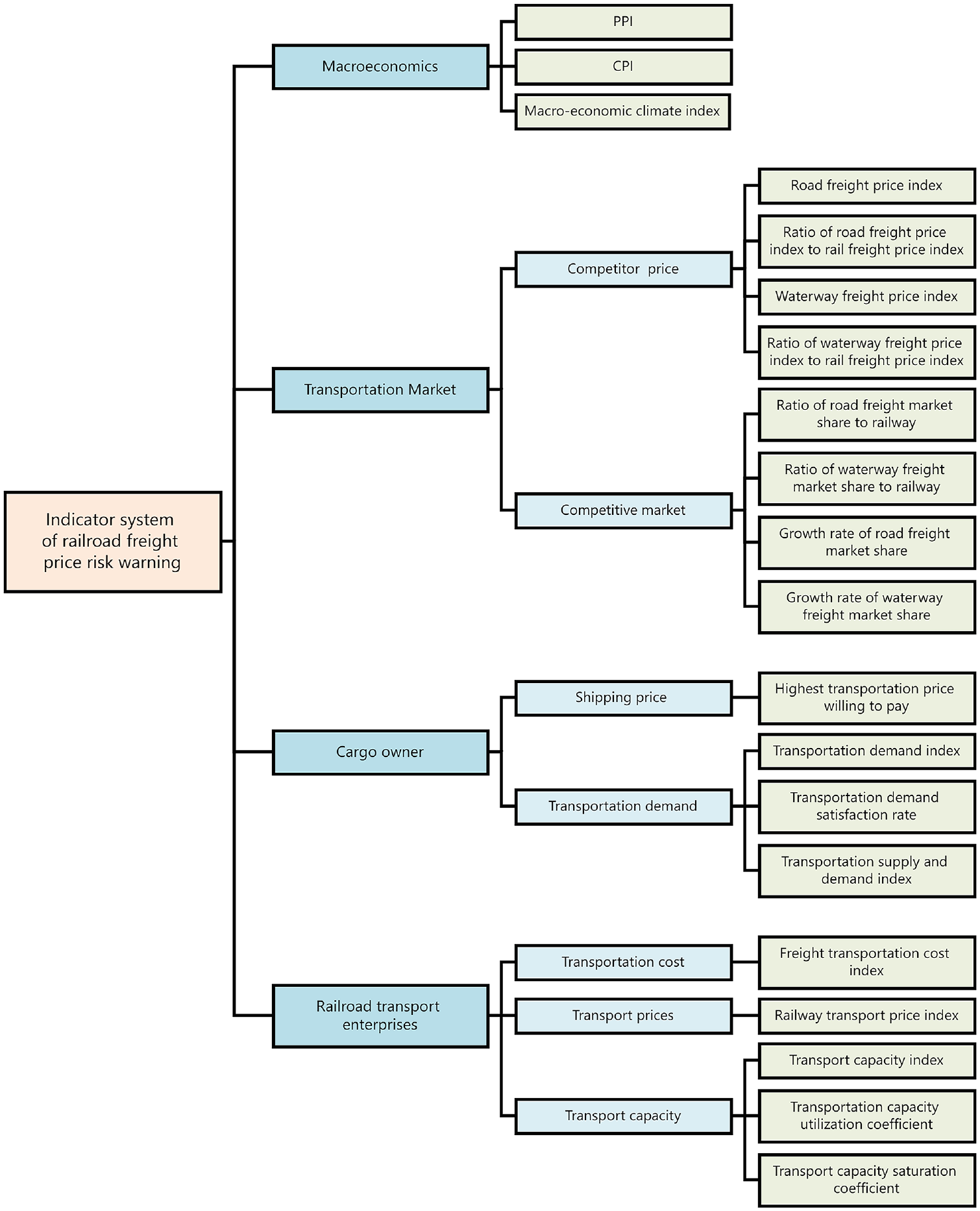
Railway freight price risk early warning index system. CPI, consumer price index; PPI, producer price index.

The following are explanations of each indicator in the index system.

Road Freight Price Index

This is a dynamic index that reflects the trends and degree of changes in road freight prices during different periods.

Ratio of Road Freight Price Index to Rail Freight Price Index

This ratio is a measure that compares the trends and extent of changes in road and rail freight prices over a certain period of time. It indicates the competitiveness of road and rail transportation in the freight market. A higher ratio suggests that road transport is relatively more expensive than rail transport, and vice versa.

Waterway Freight Price Index

This dynamic index reflects the trends and degree of changes in waterway freight rates during different periods. This article utilizes the BDI, a widely recognized international benchmark, as the waterway freight price index.

Ratio of Waterway Freight Price Index to Rail Freight Price Index

This ratio is a comparison of the waterway freight price index and the rail freight price index over time. It is calculated by dividing the waterway freight price index by the rail freight price index. If this ratio increases over time, it indicates that waterborne transport is becoming relatively more expensive than rail transport, and vice versa.

Ratio of Road Freight Market Share to Railway Freight Market Share

This indicator compares the market share of road transport with that of railroad transport. We calculate it by dividing the total freight volume of road transport by the total freight volume of rail transport. If this ratio increases over time, it indicates that road transport is gaining a larger market share than rail transport, and vice versa.

Ratio of Waterway Freight Market Share to Railway Freight Market Share

This ratio compares the market share of waterway transportation with that of railway transportation in relation to the freight volume. We calculate it by dividing the total volume of freight carried by waterway transportation by the total volume of freight carried by railway transportation. This ratio provides insight into the relative market competitiveness of waterway and railway transport modes. If the ratio is increasing over time, it suggests that waterway transportation is gaining a larger market share than railway transportation, and vice versa.

Growth Rate of Road Freight Market Share

This indicator, typically expressed as a percentage, measures the amount of change in the market share of road transport of freight over a given period of time. To calculate this indicator, we subtract the initial market share of road transport from the final market share, divide the result by the initial market share, and multiply the quotient by 100 to obtain a percentage.

Growth Rate of Waterway Freight Market Share

This indicator quantifies the change in market share of waterborne transport in relation to freight volumes over a given time period, usually expressed as a percentage. It shows how much the market share of waterborne transport has increased or decreased compared with other freight modes during a specified time period. Appropriate planning of berth resources and optimal berth allocation ( 25 ) are key elements in achieving growth in the waterborne freight market share and improving transportation efficiency.

Highest Transportation Price Willing to Pay

In the process of setting transport prices, railroad carriers should take into account the shippers’ highest tolerance for transport price, which is measured by obtaining the highest recorded transport price per ton-kilometer charged in a given month for a specific category of bulk cargo. It serves as an index of the highest transport price that shippers are willing to pay in a given month.

Transportation Demand Index

The transportation demand index refers to the number of railroad freight cars demanded by shippers per month. When the demand index is low, it means that railroad companies occupy a smaller share of the market and need to reduce the price of railroad freight to attract more customer demand.

Transportation Demand Satisfaction Rate

This rate is determined by comparing the actual number of rail freight cars loaded in a month to the number of cars demanded in the month. When the demand satisfaction rate is low, it means that railroad transport enterprises are unable to meet the transport market demand for cargo transport services. This indicates a tight capacity in railroad freight, necessitating potential price increases and a reinforcement of transport scheduling capacity to seize more market opportunities.

Transportation Supply and Demand Index

This index represents the rate of change in the monthly supply-to-demand ratio. The supply-to-demand ratio is the ratio of the maximum number of railcars available per month to the number of railcars demanded. It serves as an economic trend, reflecting the state of railroad cargo transportation services. When the transportation supply and demand index is lower, it indicates more intense competition in railroad freight transportation. In response, railroad companies should consider reducing prices to cope with the market competition.

Freight Transportation Cost Index

The purchase index of fuel power is utilized to represent the cost of railroad transportation. When setting tariffs, railroad enterprises consider the issue of transport costs as a significant factor. Given the intricate composition of railroad transport costs, it is not entirely feasible to enumerate all components, considering the operability of the index. In actual transportation, the fuel power procurement cost often occupies more than 50% of railway transportation expenses; therefore, in this work, we select the fuel power purchase index to reflect the cost of railroad transportation.

Railway Transport Price Index

This index reflects the trends of railroad freight rates across different periods. In this study, we use the monthly coal transportation invoice data of railroad bulk freight from S Railway Bureau, which encompasses the freight prices listed in each freight bill. We calculate the ratio of the average freight rate for the current month to the average freight rate for the previous month using the arithmetic mean method. We use this ratio as the current month’s railroad bulk freight rate index.

Transport Capacity Index

This index signifies the rate of change in rail freight volume for a given month. When the freight volume increases, by comparison with the previous month, it indicates an augmentation in the market share and an increase in the competitiveness of railroad companies, potentially allowing for an increase in the price of railroad transportation. Conversely, if the freight volume decreases, the price of rail transportation should be adjusted down.

Transportation Capacity Utilization Coefficient

The transportation capacity utilization coefficient reflects the full loading ratio of railroad freight cars, specifically the ratio of the actual load of railroad cars to their maximum load. If the capacity utilization coefficient is low, it means that the rail transport freight volume is relatively insufficient. In such cases, the transport price should be reduced to improve the competitiveness and attract more rail freight volume.

Transport Capacity Saturation Coefficient

The transport capacity saturation coefficient is a measure of the proportion of currently utilized railcars compared with the total number of railcars owned by the railroad company. When the capacity saturation coefficient is higher, it indicates a stronger competitive advantage in the transportation market, allowing for appropriate price increases to achieve higher transportation profits. Conversely, transport prices would be lowered to secure more market opportunities.

Method for Calculating Comprehensive Price Risk Warning Index Based on the Integrated Entropy Weighting Method and TOPSIS Method

In this work, we integrate the entropy weighting method with the TOPSIS method to derive a comprehensive early warning index for the railway bulk freight price risk. The basic idea is to initially generate new data using the entropy weighting method (where the data intrinsically become the weights calculated by the entropy weighting method), and subsequently employ the new data for the TOPSIS method study. To accurately uncover the relationships between indicators, in this work the entropy weighting method is adopted to determine the weights within the railroad tariff risk warning indicator system. It is an objective weighting method, and its objectivity stems from its being solely grounded in the inherent discreteness of the data. The greater the discreteness of the indicators, the more significant their effect on the comprehensive evaluation (weight), thereby minimizing the influence of human factors. Compared with other subjective methods, such as analytic hierarchy processes, it offers a certain degree of accuracy.

In addition, there are other objective weighting methods, such as the Criteria Importance Through Intercriteria Correlation (CRITIC) weighting method, the information weighting method, and the independence weighting method. The CRITIC weighting method comprehensively considers both data fluctuation and correlation between indicators, making it suitable for analyzing data with some correlation and the volatility of indicators themselves. However, the data within the indicator system established in this work do not exhibit strong correlation, thus rendering the CRITIC weighting method less suitable. The information weighting method is applicable for treating data variability as a kind of information and employing the degree of data volatility to measure indicator weights. The variability of the individual data within the system of indicators established in this paper is not significant enough to warrant use of the information weighting method. The independence weighting method is applicable to the calculation of weights of indicators that exhibit some inherent correlation and belong to the same system. The data within the indicator system set established in this paper lack strong correlation and thus the independence weighting method is unsuitable.

The entropy weighting method is used to determine indicator weights based on the degree of change in each index value, making it well-suited for the calculation of weights when there are many bottom-level indicators. The indicator system devised in this paper consists of 20 indicators in the bottom level (second layer), and therefore satisfies this criterion. Furthermore, there exist variations among the data indicators. Therefore, the entropy weight method was chosen to calculate weights within the early warning indicator system for railroad freight price risk.

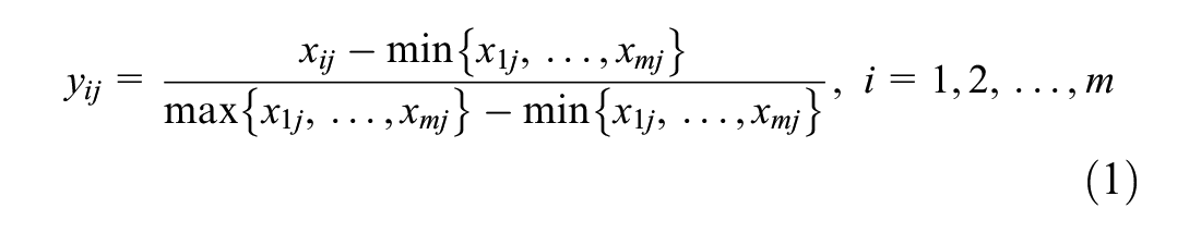
In this paper, we describe a methodology for determining weights using the entropy weighting method as follows. Before standardizing the indicator data, it is necessary to determine the positive and negative correlations between the indicators and railroad tariffs, as well as identifying positive and negative indicators. The growth of positive indicators will contribute to the increase of railway tariffs. These indicators include road and waterway tariff indexes, consumer price indexes, and so forth. Conversely, the growth of negative indicators will lead to a reduction in railroad tariffs. Examples of these negative indicators are the ratios of road and waterway market shares to the railroad market share, as well as the growth rate of road and waterway market shares. We employ the (0, 1) standardization method, assuming that the jth original indicator data value in the ith month is represented as $x_{ij}$ and the corresponding normalized index value is denoted $y_{ij}$ .

The positive index is calculated as

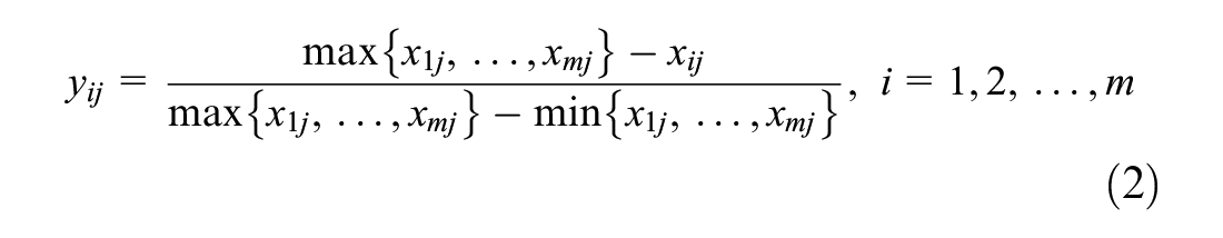
y_{i j} = \frac{x_{i j} - \min {x_{1 j}, \dots, x_{m j}}}{\max {x_{1 j}, \dots, x_{m j}} - \min {x_{1 j}, \dots, x_{m j}}}, i = 1, 2, \dots, m

(1)

The negative index is calculated as

y_{i j} = \frac{\max {x_{1 j}, \dots, x_{m j}} - x_{i j}}{\max {x_{1 j}, \dots, x_{m j}} - \min {x_{1 j}, \dots, x_{m j}}}, i = 1, 2, \dots, m

(2)

Then, the information entropy is calculated for each indicator. To begin, the proportion of the jth index value for the ith month, denoted $p_{ij}$ , is calculated:

p_{i j} = \frac{y_{i j}}{\sum_{i = 1}^{m} y_{i j}}, i = 1, 2, \dots, m, j = 1, 2, \dots, n

(3)

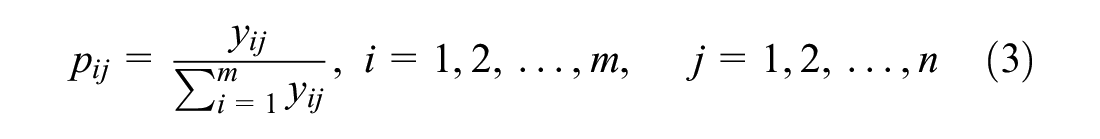
The information entropy of the jth index is calculated as $e_{j}$ :

e_{j} = - k \sum_{i = 1}^{m} p_{ij} \ln p_{ij}, i = 1, 2, \dots, m, j = 1, 2, \dots, n

(4)

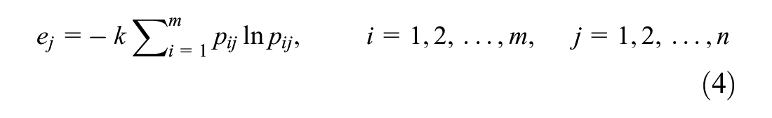
where k is a constant; commonly $k = 1 / \ln m$

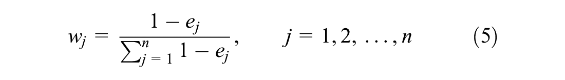
Next, the weight of the index, $w_{j}$ , is calculated:

w_{j} = \frac{1 - e_{j}}{\sum_{j = 1}^{n} 1 - e_{j}}, j = 1, 2, \dots, n

(5)

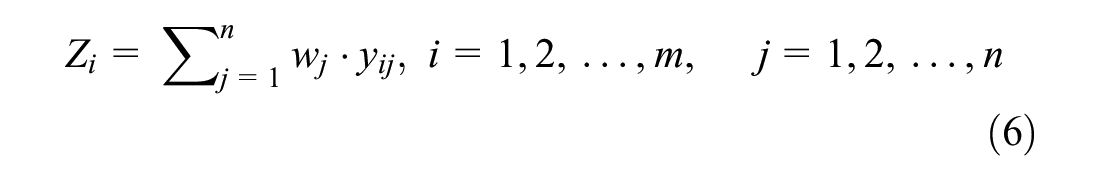
The score Z of the railway freight rate is obtained by weighting and summing the indicators, using the formula

Z_{i} = \sum_{j = 1}^{n} w_{j} \cdot y_{i j}, i = 1, 2, \dots, m, j = 1, 2, \dots, n

(6)

The TOPSIS method is a commonly employed comprehensive evaluation method that makes full use of the information within the raw data, ensuring that the results accurately reflect the gaps between evaluation programs. The following is a description of how the TOPSIS method is specifically employed to derive a comprehensive early warning index for freight price risk.

The value of $Z_{i}$ falls within the range [0, 1], and a large or small value of $Z_{i}$ indicates a high or low freight rate in the month in question. Obviously, freight rates that are too high or too low are not conducive to the development of railway enterprises. Therefore, the basis for assessing the degree of risk involves utilizing the distance between each data point, $Z_{i}$ , and the center point (centroid) of the sequence. Moreover, the centroid of this sequence is specified as the ideal solution to the TOPSIS method calculation. In this work, the sequence data Z are calculated separately and in one dimension. As a result, the multidimensional Euclidean distance method in TOPSIS is not used to calculate the distance difference between the data points and the center of the sequence (centroid). Additionally, there is no explicit method to determine the worst solution for the sequence data; thus, the worst solution distance values are not selected for calculation in this work. Therefore, the absolute value of the direct difference between each data point and the center of the series (centroid) is used as a comprehensive warning index, $Q_{i}$ :

Q_{i} = | Z_{i} - \frac{\max {Z_{1}, \dots, Z_{m}} + \min {Z_{1}, \dots, Z_{m}}}{2} |, i = 1, 2, \dots, m

(7)

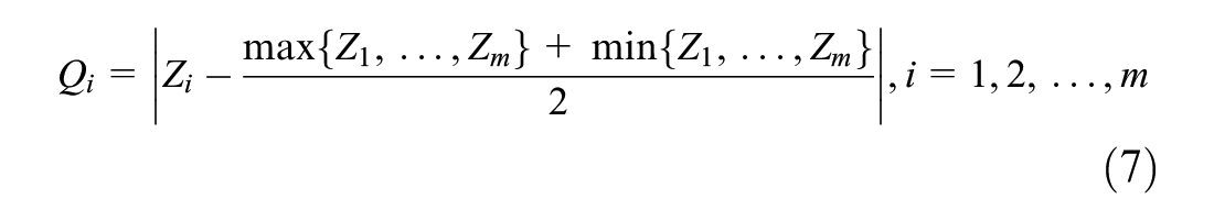
The larger the distance, the greater the comprehensive warning index $Q_{i}$ , and consequently, the higher the freight price risk; and vice versa.

Risk Warning Classification Based on k-Means Clustering Method

Currently, there is no specific methodological reference for setting an early warning range for rail freight transport prices. We define price risk as the risk of rail freight prices being too high or too low. In this paper, we propose use of the k-means clustering method to categorize a comprehensive early warning index for the price risk of railway bulk cargo transportation. This classification encompasses five distinct early warning levels: no risk, low risk, medium risk, high risk, and very high risk. The k-means algorithm is a clustering algorithm that focuses on the grouping and categorization of data using the Manhattan distance. This distance is calculated directly, since the comprehensive warning index is one-dimensional. Based on the comprehensive early warning index $Q_{i}$ calculated in Equation 7, it is then classified into five levels. The basic steps are as follows.

Step 1: Randomly select k samples as the initial cluster centers for classification, denoted $C = (C_{1}, C_{2}, \dots, C_{k})$ .

Step 2: Calculate the Manhattan distance between each sample $Q_{i}$ and the k clustering centers; then assign the sample to the cluster with the closest distance to its center. The formula for calculating the Manhattan distance between points $Q = (Q_{1}, Q_{2}, \dots, Q_{m})$ and $C = (C_{1}, C_{2}, \dots, C_{k})$ is

d (Q_{i}, C_{j}) = | Q_{i} - C_{j} |, 1 \leq i \leq m, 1 \leq j \leq k

(8)

Step 3: After the classification is completed, the mean of all samples in each cluster is calculated as the new clustering center $C_{j}$ :

C_{j} = \frac{1}{v_{j}} \sum_{Q_{i} \in u_{j}} Q_{i}, j = 1, 2, \dots, k, i = 1, 2, \dots, m

(9)

Here, the number of samples in each cluster $u_{1}, u_{2}, \dots, u_{k}$ is assumed to be $v_{1}, v_{2}, \dots, v_{k}$ .

Step 4: Repeat steps 2 and 3 until a termination condition (such as several iterations or an error requirement) is reached.

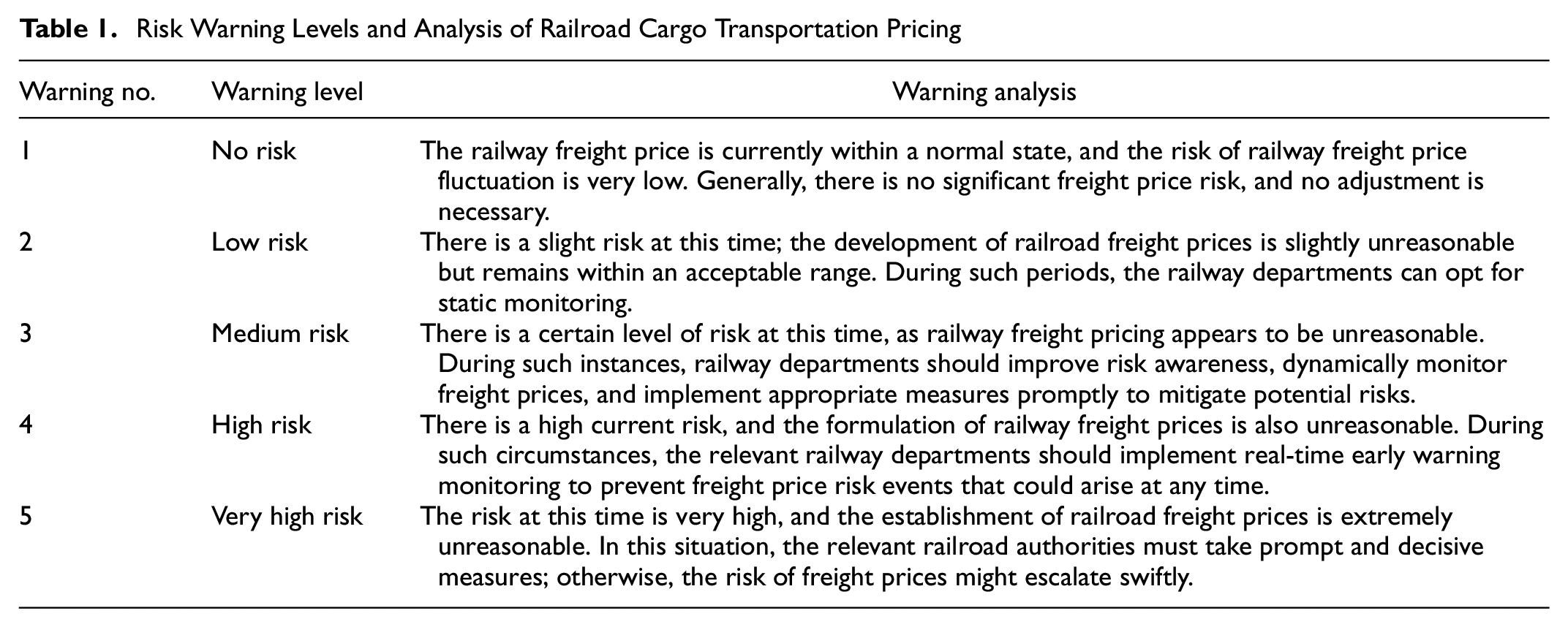
The cluster center values, arranged from small to large, correspond to the five risk warning levels identified previously. The specific risk analyses corresponding to these five risk level classes are shown in Table 1.

Table 1.

Risk Warning Levels and Analysis of Railroad Cargo Transportation Pricing

Warning no.	Warning level	Warning analysis
1	No risk	The railway freight price is currently within a normal state, and the risk of railway freight price fluctuation is very low. Generally, there is no significant freight price risk, and no adjustment is necessary.
2	Low risk	There is a slight risk at this time; the development of railroad freight prices is slightly unreasonable but remains within an acceptable range. During such periods, the railway departments can opt for static monitoring.
3	Medium risk	There is a certain level of risk at this time, as railway freight pricing appears to be unreasonable. During such instances, railway departments should improve risk awareness, dynamically monitor freight prices, and implement appropriate measures promptly to mitigate potential risks.
4	High risk	There is a high current risk, and the formulation of railway freight prices is also unreasonable. During such circumstances, the relevant railway departments should implement real-time early warning monitoring to prevent freight price risk events that could arise at any time.
5	Very high risk	The risk at this time is very high, and the establishment of railroad freight prices is extremely unreasonable. In this situation, the relevant railroad authorities must take prompt and decisive measures; otherwise, the risk of freight prices might escalate swiftly.

After determining the comprehensive warning index and price risk warning level for the rail bulk transport price risk for each month, the subsequent step is to utilize these comprehensive warning index data with time series characteristics. We employ different neural network methods to predict the comprehensive warning indexes and risk warning levels for future periods and to verify which neural network prediction method is more accurate.

LSTM-Based Prediction Method for Railroad Bulk Freight Price Risk and Performance Evaluation

For the prediction of comprehensive warning indexes of railroad bulk cargo price risk, neural network methods or other time series prediction methods can be used. In this work, we aim to utilize both the BP neural network model proposed by Rumelhart et al. ( 26 ) and the LSTM neural network model proposed by Hochreiter and Schmidhuber ( 27 ) to construct an alternative set of comprehensive early warning index prediction models. Subsequently, the parameters of these two neural network methods will be optimized and adjusted to achieve better prediction accuracy for the comprehensive early warning index of railroad bulk cargo transportation price risk.

Setting Parameters for LSTM and BP Neural Networks

Training the BP neural network and deep learning LSTM neural network involves configuring many parameters. Selecting the correct values for each parameter can be challenging. A common method is to set the value range of parameters based on everyone’s experience and then combine different parameters according to the value range of each parameter to create various possible parameter combinations. Subsequently, we perform the training operation according to the built-in model algorithm in the neural network. Because the neural network training uses random values, each training run yields different results. To determine the optimal parameter configuration, we need to perform many training operations to attain the most stable and optimal calculation results. This section is based on continuous experimental testing during the neural network training process. The aim is to identify the best parameter settings for both the BP neural network and LSTM neural network, leading to the most optimized and stable training results. The neural network training results of these optimized parameter configurations will meet the prediction accuracy requirements of comprehensive early warning indexes.

Setting Parameters for the BP Neural Network

The BP neural network follows a typical three-layer BP neural network structure, which consists of an input layer, a hidden layer, and an output layer. Steps 1 through 4 provide a guideline for setting the parameters of a BP neural network for a railway freight price risk early warning model.

1. Determine the number of input nodes.

The number of input nodes of the neural network is determined based on the specific problem to be addressed. For the railway freight price risk early warning model proposed in this paper, the input consists of the number of monthly indicators, which is 20.

2. Determine the number of output nodes.

The output of the neural network is the comprehensive early warning index of the next month, and the corresponding output node number is set to 1.

3. Determine the numbers of hidden layers and hidden neurons.

For the BP neural network, the empirical formula is used to determine the appropriate number of neurons in the hidden layer:

N = \sqrt{I + O} + b

(10)

where $N$ represents the number of nodes in the hidden layer, $I$ and $O$ denote the numbers of nodes in the input and output layers, respectively, and $b$ is a regulation constant, taking values between 1 and 10. In this case, the value of the number of nodes in the hidden layer $(N)$ is set to 13.

4. The sigmoid function is a common activation function in BP neural networks. It is characterized by the continuity of both the function itself and its derivatives, making it very easy to handle. We have selected the sigmoid function as the activation function of the BP neural network.

Optimal Setting of Deep Learning LSTM Neural Network Parameters

The LSTM neural network is an enhanced type of recurrent neural network designed to excel in detecting long-term dependencies within data. Graves ( 28 ) refined and popularized the LSTM architecture. This neural network model incorporates a memory cell structure to record the state of neurons, along with input, output, and forgetting gates to control the retention and removal of information within the neurons. The LSTM neural network facilitates long-term memory within the network through the introduction of gate mechanisms. 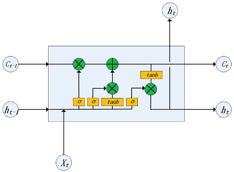Figure 2 shows the structure of an LSTM neural network, where multiplication is denoted $by \otimes$ , addition $by \oplus$ , $C$ signifies long-term memory, $h$ represents short-term or working memory, $X_{t}$ denotes the feature vector at moment $t$ , and $σ$ represents the activation function.

Figure 2.

Long short-term memory (LSTM) neural network structure.

In a deep learning LSTM neural network, a series of parameter adjustment and comparison experiments is conducted to select the best configuration parameters. The aim in this process is to achieve the best accuracy of the network prediction results while minimizing errors. The hyperparameter settings of the LSTM neural network in this work are as follows: the number of input nodes is 20, the number of output nodes is 1, and there are two hidden layers with 128 hidden layer nodes. The time step is 3, the dropout rate is 0.5, the mean square error is used as the loss function, there are 500 epochs, tanh is used as the activation function, and the Adam optimizer is utilized.

Performance Evaluation Metrics for LSTM and BP Neural Network Methods

The symmetric mean absolute percentage error (SMAPE) and the root mean square error (RMSE) are used to assess the predictive performance of the network; in addition, the coefficient of determination $R^{2}$ is used to measure the degree of curve fitting.

The SMAPE is defined as

SMAPE = \frac{100 %}{n} \sum_{i = 1}^{n} \frac{| Q_{i}^{*} - Q_{i} |}{(| Q_{i}^{*} | + | Q_{i} |) / 2}

(11)

The RMSE is defined as

RMSE = \sqrt{\frac{\sum_{i = 1}^{n} {(Q_{i} - Q_{i}^{*})}^{2}}{n}}

(12)

The function expression of the coefficient of determination is calculated as

R^{2} = 1 - \frac{\sum_{i = 1}^{n} {(Q_{i} - Q_{i}^{*})}^{2}}{\sum_{i = 1}^{n} {(Q_{i} - Q_{0})}^{2}}

(13)

where

$Q_{i}$ : actual value of comprehensive warning index in ith month

$Q_{i}^{*}$ : predictive value of comprehensive warning index in ith month

$Q_{0}$ : average of actual value of comprehensive warning index

$n$ : total number of tests

Smaller values of SMAPE and RMSE indicate smaller errors in the system, resulting in better prediction accuracy. A higher value of the determination coefficient R² indicates a better fit between the predicted network value and the actual value.

Case Analysis

Analysis of Bulk Cargo Freight Ticket Data from S Railway Bureau

For this study, a total of 8,301,528 cargo ticket records from the S Railway Bureau, spanning from 2015 to 2017, were collected. The dataset primarily comprises 10 cargo categories, including coal, gold mines, and steel. Notably, coal transportation holds a major position, accounting for 43.33% of the total cargo volume across all categories. Consequently, this section focuses on the transportation price of coal as the primary research object.

Railway transportation is well-suited for long-distance cargo transport; it becomes advantageous at distances from 800 km. When the goods transportation distance falls within the range 800–1500 km, the competition between road transportation and railway transportation becomes notably intense. Consequently, we have compiled and organized the coal transportation data covering distances of 800 to 1500 km from the S Railway Bureau for the following analysis.

Data Preprocessing and Risk Warning Level Division

Data Normalization

In this article work, coal transportation data from the S Railway Bureau, spanning the years 2015 to 2017, are utilized as an example for analysis. The source data originate from the S Railway Bureau, the National Bureau of Statistics, the China Federation of Logistics and Purchasing, and so forth. The data are segmented into 36 months, on a monthly basis. To comply with the data input requirements of the BP and LSTM neural network conversion functions, the 36-month raw index data are normalized. The chosen normalization method is the (0, 1) standardization method:

Y_{i} = \frac{X_{i} - X_{min}}{X_{max} - X_{min}}

(14)

where

$Y_{i}$ : normalized result of data point i

$X_{i}$ : actual value of data point i

$X_{min}$ : minimum value of data set

$X_{max}$ : maximum value of data set

Index Weight Calculation and Risk Warning Division

We use the entropy weighting method mentioned previously to calculate the weightings for each indicator within the railroad bulk cargo transportation price risk warning indicator system. The calculated weightings for each indicator are presented in Table 2.

Table 2.

Weighting of Each Indicator

Indicator	Weighting	Indicator	Weighting
Producer price index	0.056	Ratio of road freight price index to railway freight price index	0.085
Consumer price index	0.035	Waterway freight price index	0.034
Macroeconomic climate index	0.070	Ratio of waterway freight price index to rail freight price index	0.043
Road freight price index	0.076	Ratio of road freight market share to railway freight market share	0.052
Ratio of waterway freight market share to railway freight market share	0.039	Growth rate of road freight market share	0.019
Growth rate of waterway freight market share	0.017	Highest transportation price willing to pay	0.021
Transportation demand index	0.071	Transportation supply and demand index	0.142
Transportation demand satisfaction rate	0.024	Freight transportation cost index	0.036
Railway transport price index	0.025	Transport capacity index	0.105
Transportation capacity utilization coefficient	0.022	Transport capacity saturation coefficient	0.029

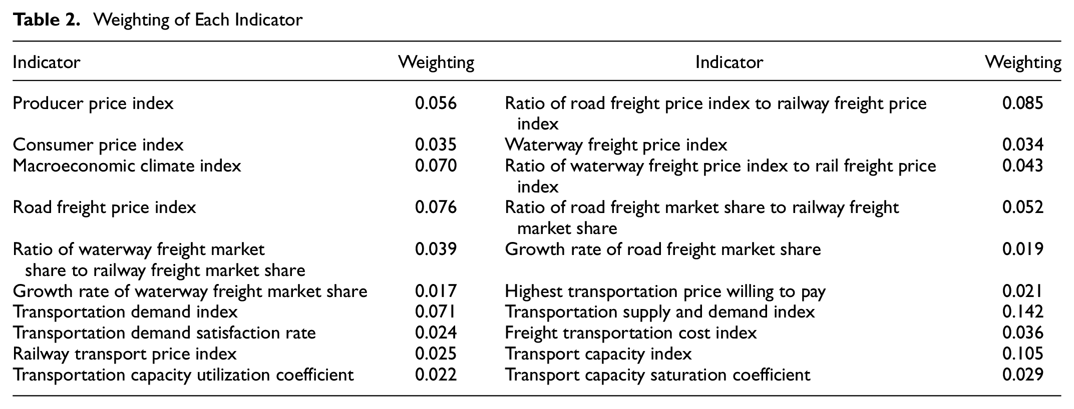
Subsequently, we multiply the monthly data of indicators that influence railway freight rates by their respective weightings to derive the evaluation scores. With these evaluation scores, we apply the TOPSIS method, as defined in this study, to calculate the comprehensive price risk warning index values for each month spanning from 2015 to 2017. The results are illustrated in Figure 3. Utilizing PyCharm software and the k-means clustering algorithm, we identified five clustering centers, at 0.0392, 0.1947, 0.4124, 0.5959, and 0.9084, corresponding to clusters 1, 2, 3, 4, and 5, respectively.

Figure 3.

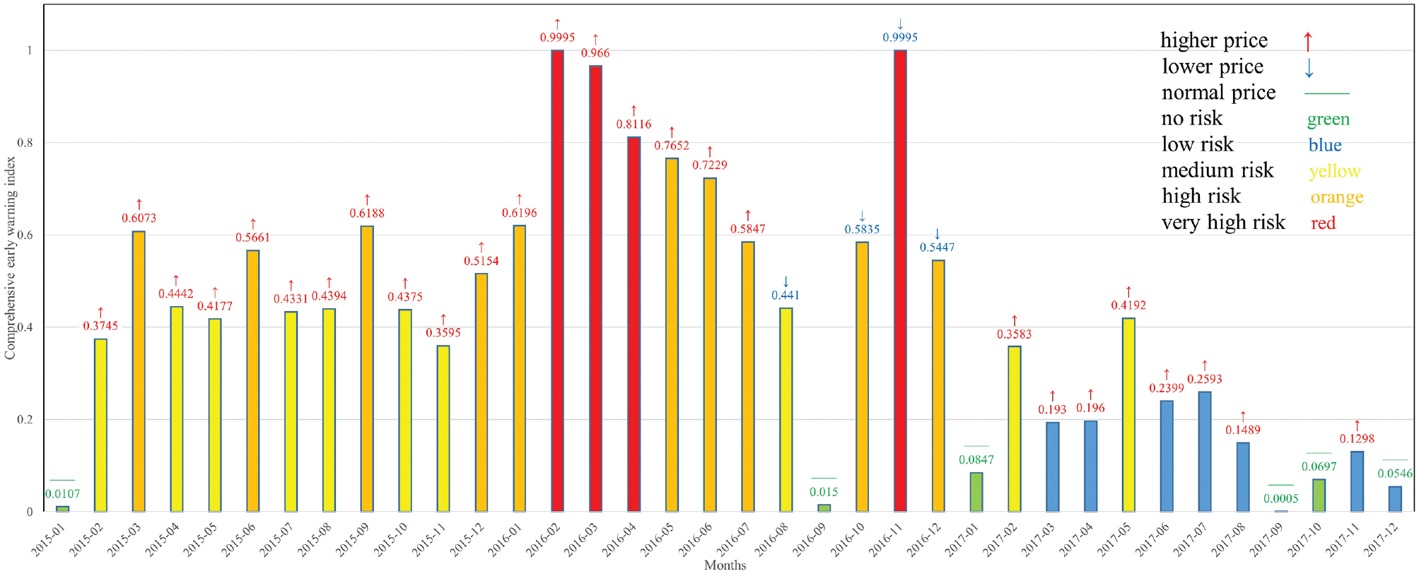
S Railway Bureau’s risk warning for each month from 2015 to 2017.

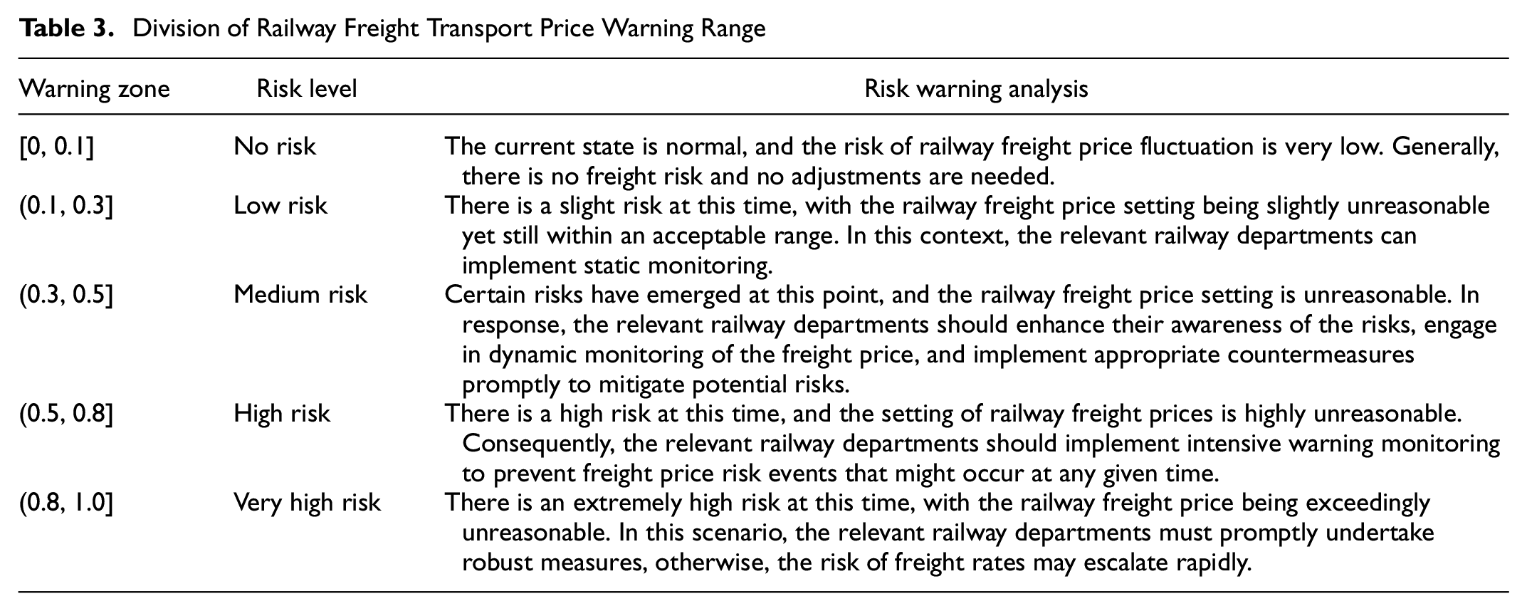
There is no definitive standard for categorizing freight risk within the railway industry. In this work, we integrate the classification results of the k-means clustering method, along with expert opinions, pertinent literature on railway freight price evaluation, and the risk warning degree classification method used for economic climate indexes.

Considering the operational context of the S Railway Administration, we divided the risk alarm levels into five categories: no risk, low risk, medium risk, high risk, and very high risk.

Table 3 presents the specific interval divisions and risk warning analysis.

Table 3.

Division of Railway Freight Transport Price Warning Range

Warning zone	Risk level	Risk warning analysis
[0, 0.1]	No risk	The current state is normal, and the risk of railway freight price fluctuation is very low. Generally, there is no freight risk and no adjustments are needed.
(0.1, 0.3]	Low risk	There is a slight risk at this time, with the railway freight price setting being slightly unreasonable yet still within an acceptable range. In this context, the relevant railway departments can implement static monitoring.
(0.3, 0.5]	Medium risk	Certain risks have emerged at this point, and the railway freight price setting is unreasonable. In response, the relevant railway departments should enhance their awareness of the risks, engage in dynamic monitoring of the freight price, and implement appropriate countermeasures promptly to mitigate potential risks.
(0.5, 0.8]	High risk	There is a high risk at this time, and the setting of railway freight prices is highly unreasonable. Consequently, the relevant railway departments should implement intensive warning monitoring to prevent freight price risk events that might occur at any given time.
(0.8, 1.0]	Very high risk	There is an extremely high risk at this time, with the railway freight price being exceedingly unreasonable. In this scenario, the relevant railway departments must promptly undertake robust measures, otherwise, the risk of freight rates may escalate rapidly.

We assigned the comprehensive risk warning index of freight rates for the S Railway Bureau for each month spanning from 2015 to 2017 to the corresponding early warning level, based on the early warning levels delineated in Table 3. The results are presented in Figure 3. The data source for Figure 3 has been mentioned in the previous subsection.

Figure 3 reflects changes in the comprehensive freight price warning index, the level of price risk rating, and the direction of price risk over 36 months. The following is an analysis of the main factors influencing price risk.

January and February 2015: The comprehensive freight price early warning index increased from the no-risk warning level to the medium-risk warning level of excessive price in February 2015. Because the Chinese Government decided to increase the national average rail freight rate by 1 cent/ton-km (RMB 0.01/ton-km), from 14.51 cents to 15.51 cents, effective February 1, 2015, rail freight price risk rose from no risk to medium risk, and rail freight volume fell by 13.9% in February 2015.

February 2015 to February 2016: There was no essential change in rail freight prices. Monthly rail freight volumes decreased significantly compared with the same period in the previous year, and monthly price risk was in the range of medium to high. The risk became very high by February 2016.

March 1, 2016: The Chinese Government reduced the benchmark price of rail freight from RMB 0.098/ton-km to RMB 0.088/ton-km, in response to the competition in road transport and the loss of cargo sources. The rate of decline in rail freight volumes slowed significantly in March 2016, dropping back to 4.1% from 9.1% in February. However, the level of freight rates remained high, and price risk remained at a very high level. This situation continued without improvement until July 2016.

August 30, 2016: The situation started to improve. China’s Ministry of Transport issued Management Measures on the Management of Over-Limit Transportation Vehicles Driving on Highways and Over-Limit Trucks on Highways, leading to a rise in road transport prices from August 2016 to the beginning of 2017. This gave railroad transportation a strong competitive advantage over road transportation, and freight volumes began to pick up gradually. The price risk shifted from too high to too low, and the level of too-low price risk was in the medium-risk range.

October 2, 2016: Rail freight prices began to increase as the Chinese Government restored the benchmark price of rail freight from RMB 0.088/ton-km to RMB 0.098/ton-km. This was a result of the stabilization of the economy and the increase in demand for coal shipments, which led to a substantial rebound in demand for railroad coal transportation and a tightening of railroad capacity. However, the price of rail freight remained too low. The very high-risk level of too-low prices was reached in November 2016, while road transport prices continued to rise to near-historical peak positions during this period.

January 2017: The risk of too-low rail freight prices reduced from a high-risk level to a no-risk level as the rate of road transport price increases fell back, attributable to the continued reduction in gasoline prices.

February to May 2017: Railway freight prices began to approach the warning level of too-high prices, while road transport prices had decreased by 7.6% compared with January. By May 2017, railway freight prices reached a medium-risk level of too-high prices.

June 1, 2017: Railroad freight prices started to decrease, and the surcharge for electricity in the electrified section of the implementation of the national unified railroad tariff was reduced from RMB 0.012/ton-km to RMB 0.007/ton-km. Although, a risk of being too high persisted, the risk level remained low, effectively maintaining a basic low-level risk scenario.

Therefore, the risk classification results from the comprehensive early warning price index, shown in Figure 3, are consistent with the actual price risk conditions faced by railway enterprises. It is very important to accurately assess the early warning level for price risk in railway freight marketing. Understanding the price risk early warning level enables a railway department to proactively adapt to market dynamics. For example, when the price remains above the cost price, adjustments from a high price level to a lower one can be made. Conversely, if the price falls below the cost price, it might be possible to abandon the freight market. In the scenario of low pricing and a concurrent increase in the overall prices within the competitive transportation market, the railway enterprise can strategically respond by raising freight prices. This adjustment becomes particularly pertinent when railway transport capacity is strained. Such a move allows for the acquisition of greater benefits, serving to offset the profit loss that the railway freight enterprise might encounter during periods of lower freight pricing.

Comparison between BP and Optimally Configured LSTM Methods in Forecasting Transportation Price Risk and Early Warning Level

Firstly, the BP neural network was employed to determine the comprehensive early warning index for railway freight prices spanning from January 2015 to December 2017. The network’s input consisted of the indicator dataset from the preceding month, while the output represented the comprehensive freight rate early warning index for the month being analyzed. This input–output relationship encompassed 35 groups of corresponding data. Among these, 26 groups of data were chosen for neural network training, while the remaining 9 groups of data were reserved for neural network verification.

1. Parameter setting for BP neural network model experiment.

To enhance the input signal learning and signal convergence, we opted for the sigmoid function as the activation function for the BP neural network.

Through numerous iterative experiments on the neural network, an optimal learning rate of 0.1 was selected. Furthermore, after 10,000 iterations, the neural network tends to plateau.

2. Determining the number of neurons in the hidden layer.

According to the empirical formula method, the number of hidden layer neurons was determined to be within the range 6–15. Subsequently, using Python application software, the normalized index data were input, and the network underwent several iterations of training. This training revealed that the number of hidden layer neurons yielding the lowest system error value is 13. As a result, we determined the number of hidden layer neurons to be 13 and proceeded with subsequent training of the BP neural network.

Subsequently, we fed the remaining nine sets of data into the previously trained neural network for validation, assessing whether the neural network’s training aligned with the study’s requirements. The prediction results for these nine groups are shown in the left panel of Figure 4. Figure 4 and Table 4 give a more intuitive comparison of BP and LSTM results, showcasing the calculation outcomes of both methods.

Figure 4.

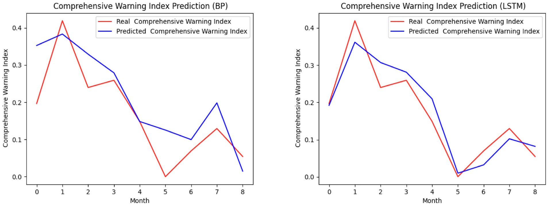
Prediction results of neural network training with back propagation (BP) and long short-term memory (LSTM) methods.

Table 4.

Back Propagation and Long Short-Term Memory Neural Network Verification Results

Number of groups	Actual value of comprehensive early warning index	Risk warning level	Back propagation			Long short-term memory
Number of groups	Actual value of comprehensive early warning index	Risk warning level	Predicted value of comprehensive warning index	Risk warning level	Difference	Predicted value of comprehensive warning index	Risk warning level	Difference
1	0.1968	Low	0.3525	Medium	0.1557	0.192	Low	−0.0048
2	0.4192	Medium	0.3833	Medium	−0.0359	0.3615	Medium	−0.0577
3	0.2399	Low	0.3292	Medium	0.0893	0.3069	Medium	0.0670
4	0.2593	Low	0.2791	Low	0.0198	0.281	Low	0.0217
5	0.1489	Low	0.1483	Low	−0.0006	0.2095	Low	0.0606
6	0.0005	No	0.1253	Low	0.1248	0.0099	No	0.0094
7	0.0697	No	0.0996	No	0.0299	0.0322	No	−0.0375
8	0.1298	Low	0.1984	Low	0.0686	0.1022	Low	−0.0276
9	0.0546	No	0.0148	No	−0.0398	0.0818	No	0.0272
Root mean square error			0.0793			0.0408
Symmetric mean absolute percentage error (%)			55.00			44.63
$R^{2}$			0.3394			0.6603

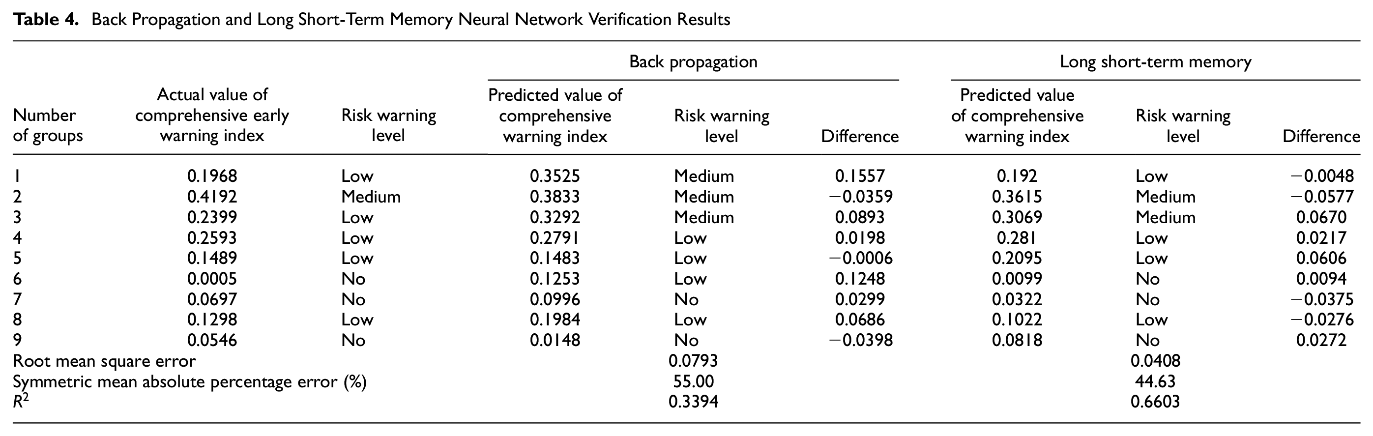
Although the prediction result curves after the model training are generally consistent with the trend of the actual values, some points deviate from the actual values by a large margin. The validation results of the BP neural network are given in Table 4.

On examining the predicted and actual values of the validation dataset after application of the neural network, noticeable disparities are observed. In relation to risk warning prediction, the BP neural network model demonstrates a prediction accuracy of 67%, which is relatively low. In pursuit of higher prediction accuracy, our subsequent experiments will utilize the LSTM deep learning network model.

The enhanced performance of the case study involving the LSTM neural network was validated by comparing the accuracy of the prediction results. The model’s input consisted of an index data collection from the preceding 3 months, while the output represented the comprehensive early warning index of the freight price rate for the subsequent month. Of the 33 groups of corresponding data, 24 groups were selected as the model’s training dataset, and the remaining 9 groups were designated as the validation dataset.

We describe the building, training, and performance evaluation of the LSTM neural network model as follows.

Parameter Setting for LSTM Neural Network Model Experiment

In configuring parameters for the LSTM neural network, two main categories arise: basic parameters and hyperparameters. Basic parameters include the determinations of weightings and bias items in the network connection layer, which are determined by the system itself. Hyperparameters, however, necessitate manual tuning, encompassing such aspects as the number of time steps, epoch, optimizer, and activation function. The specific hyperparameter settings for the LSTM neural network in this work are described in a previous subsection in this paper.

LSTM Neural Network Training

The right panel of Figure 4 presents the prediction results of the LSTM neural network. It is evident from the figure that the prediction curves of the LSTM neural network closely match the actual values, with almost all data points aligning with the curves. The fields in the LSTM section of Table 4 illustrate the validation results of the LSTM neural network. The smaller prediction error results exhibited by the LSTM neural network indicate its high prediction accuracy. The predicted risk warnings are highly aligned with the actual values, achieving an accuracy of 89%. Although the early warning prediction results in the third data set slightly deviate by one warning level from the actual warnings, the predicted values themselves remain very close to the boundaries of the warning intervals.

Comparative Performance Analysis of Early Warning Results

To provide an intuitive and accurate comparison of the predictive efficacy of the two models, we employ three evaluation methods: RMSE, SMAPE, and R². These metrics serve to assess the prediction performance of the BP neural network algorithm and the LSTM neural network algorithm. The final section of Table 4 shows the evaluation results. Notably, the RMSE for the BP neural network is 0.0793, and the corresponding SMAPE is 55.00%, whereas the RMSE for the LSTM neural network is 0.0408, with an associated SMAPE of 44.63%. The higher error values in the BP method indicate its lower accuracy, compared with the LSTM method. Additionally, R² for BP is 0.3394, while R² for the LSTM neural network is 0.6603. This discrepancy suggests that the LSTM neural network exhibits considerably better goodness-of-fit, signifying better predictive performance, compared with the BP neural network. This analysis supports the finding that the deep learning LSTM neural network, coupled with optimized parameter configuration, offers greater accuracy in predicting risk warnings for railroad freight transportation prices.

Conclusions

In this work, an advanced railroad freight price risk early warning index system was developed by meticulously selecting 20 influential factors from four different aspects: macroeconomy, transportation market, cargo owners, and railroad enterprises. We established a comprehensive price risk early warning index using the entropy weight method and the TOPSIS method. Furthermore, we utilized the k-means method to divide the comprehensive warning index into five levels of warning intervals. To enhance the precision of risk prediction and early warning level for railroad freight transportation, we constructed and assessed two distinctive neural network methods, namely the BP approach and the LSTM parameter optimization configuration technique. To verify the effectiveness of the proposed method, we drew on actual cargo ticket data sourced from China’s S Railway Bureau during the period spanning 2015 to 2017.

The study results indicate that the parameter-optimized configuration LSTM method can predict the risk level of bulk cargo freight prices more effectively and accurately than the BP neural network method. The proposed method provides theoretical support for price risk warning and price control in railroad transportation. Furthermore, the study demonstrates the significance of considering different factors affecting price risk to establish an EWS for railway cargo transportation.

In future research, we recommend the exploration of price risk control in multimodal transport, including sea–rail intermodal transport and road–rail intermodal transport, as well as other types of multimodal transport. Moreover, the prediction model’s accuracy could be enhanced by incorporating more factors that affect the interactions between cargo owners, transportation enterprises, and the transportation market. Finally, transforming the macroscopic approach of the early warning index system into a microscopic approach could also provide valuable insight into price risk warning for and control of transportation.

Footnotes

Author Contributions

The authors confirm contribution to the paper as follows: study conception and design: Jin Zeng and Shaoyuan Guo; data collection: Jin Zeng, Shaoyuan Guo, and Jinhao Zeng; analysis and interpretation of results: Jin Zeng, Shaoyuan Guo, and Kehuai Jin; draft manuscript preparation: Jin Zeng and Shaoyuan Guo. All authors reviewed the results and approved the final version of the manuscript.

Declaration of Conflicting Interests

The author(s) declared no potential conflicts of interest with respect to the research, authorship, and/or publication of this article.

Funding

The author(s) disclosed receipt of the following financial support for the research, authorship, and/or publication of this article: This research was supported by the Fundamental Research Funds for the Central Universities (grant number 2021PT207).

ORCID iDs

Jin Zeng

Shaoyuan Guo

Jinhao Zeng

Data Accessibility Statement

The data used in this study are not accessible.

References

Bruinshoofd

Candelon

Raabe

Banking Sector Fragility and the Transmission of Currency Crises. Open Economies Review, Vol. 21, No. 2, 2010, pp. 263–292.

Guo

Shen

The Impact of Internet Finance on Commercial Banks’ Risk Taking: Evidence from China. China Finance and Economic Review, Vol. 4, No. 1, 2016, pp. 1–19.

Fletcher

Shawe-Taylor

Multiple Kernel Learning with Fisher Kernels for High Frequency Currency Prediction. Computational Economics, Vol. 42, No. 2, 2013, pp. 217–240.

Amédée-Manesme

C. O.

Barthélémy

Keenan

Cornish-Fisher Expansion for Commercial Real Estate Value at Risk. The Journal of Real Estate Finance and Economics, Vol. 50, No. 4, 2015, pp. 439–464.

Golbabai

Mohebianfar

A New Stable Local Radial Basis Function Approach for Option Pricing. Computational Economics, Vol. 49, No. 2, 2017, pp. 271–288.

Witkowska

Discrete Choice Model Application to the Credit Risk Evaluation. International Advances in Economic Research, Vol. 12, No. 1, 2006, pp. 33–42. https://doi.org/10.1007/s11294-006-6124-0.

Moradi

Rafiei

F. M.

A Dynamic Credit Risk Assessment Model with Data Mining Techniques: Evidence from Iranian Banks. Financial Innovation, Vol. 5, No. 1, 2019, pp. 1–27.

Abid

Masmoudi

Zouari-Ghorbel

The Consumer Loan’s Payment Default Predictive Model: An Application of the Logistic Regression and the Discriminant Analysis in a Tunisian Commercial Bank. Journal of the Knowledge Economy, Vol. 9, No. 3, 2018, pp. 948–962.

Santarelli

The Duration of New Firms in Banking: An Application of Cox Regression Analysis. Empirical Economics, Vol. 25, No. 2, 2000, pp. 315–325.

10.

Mumtaz

M. Z.

Smith

Z. A.

IPO Cycles in Pakistan. Borsa Istanbul Review, Vol. 21, No. 4, 2021, pp. 405–417.

11.

Yanhong

Listed Company Financial Risk Prediction Based on BP Neural Work. Proc., 7th International Conference on Measuring Technology and Mechatronics Automation, Nanchang, China, IEEE, New York, 2015, pp. 601–604.

12.

Zhang

A Credit Risk Assessment Model Based on SVM for Small and Medium Enterprises in Supply Chain Finance. Financial Innovation, Vol. 1, No. 1, 2015, pp. 1–21.

13.

Leong

C. K.

Credit Risk Scoring with Bayesian Network Models. Computational Economics, Vol. 47, No. 3, 2016, pp. 423–446.

14.

Kaminsky

Lizondo

Reinhart

C. M.

Leading Indicators of Currency Crises. Staff Papers, Vol. 45, No. 1, 1998, pp. 1–48.

15.

Shi

Gao

A Study on KLR Financial Crisis Early-Warning Model. Frontiers of Economics in China, Vol. 5, No. 2, 2010, pp. 254–275.

16.

Xie

Han

Multi-Factor RFG-LSTM Algorithm for Stock Sequence Predicting. Computational Economics, Vol. 57, No. 4, 2021, pp. 1041–1058.

17.

Yıldırım

D. C.

Toroslu

I. H.

Fiore

Forecasting Directional Movement of Forex Data Using LSTM with Technical and Macroeconomic Indicators. Financial Innovation, Vol. 7, No. 1, 2021, pp. 1–36.

18.

Yang

Dong

Ogandaga

Forewarning of Freight Rate in Shipping Market Based on Support Vector Machine. In Traffic and Transportation Studies ( Mao

Tian

Huang

Gao

, eds.), American Society of Civil Engineers, Reston, VA, 2008, pp. 295–303.

19.

Chen

Luo

An Early-Warning System for Shipping Market Crisis Using Climate Index. Journal of Coastal Research, Vol. 73(10073), 2015, pp. 620–627.

20.

Yun

J.-N.

Kim

G.-H.

Ryoo

D.-K.

A Study on Early Warning Model in the Dry Bulk Shipping Industry by Signal Approach. Journal of Navigation and Port Research, Vol. 42, No. 1, 2018, pp. 57–66.

21.

Choi

J. S.

Kim

K. H.

Han

H. J.

Development of Early Warning Index in Korean Shipping Industry by Using Signal Approach. Maritime Policy & Management, Vol. 45, No. 8, 2018, pp. 1007–1020.

22.

Haji-Kazemi

Andersen

Krane

H. P.

Identification of Early Warning Signs in Front-End Stage of Projects, an Aid to Effective Decision Making. Procedia—Social and Behavioral Sciences, Vol. 74, 2013, pp. 212–222.

23.

Gao

Zhang

Peng

Hao

Study on the Relationship Between Comprehensive Transportation Freight Index and GDP in China. Procedia Engineering, Vol. 137, 2016, pp. 571–580.

24.

Zeng

Guo

Zeng

Comprehensive Evaluation Model and Empirical Research on Railway Freight Rates in a Competitive Environment. Transportation Research Record: Journal of the Transportation Research Board, 2021. 2675: 929–938.

25.

Tang

Fang

S. S.

Discretization-Strategy-Based Solution for Berth Allocation and Quay Crane Assignment Problem. Journal of Marine Science and Engineering, Vol. 10, No. 4, 2022, p. 495.

26.

Rumelhart

D. E.

Hinton

G. E.

Williams

R. J.

Learning Representations by Back-Propagating Errors. Nature, Vol. 323, No. 6088, 1986, pp. 533–536.

27.

Hochreiter

Schmidhuber

Long Short-Term Memory. Neural Computation, Vol. 9, No. 8, 1997, pp. 1735–1780.

28.

Graves

Supervised Sequence Labelling. In Supervised Sequence Labelling with Recurrent Neural Networks ( Graves

, ed.), Springer, Berlin, Heidelberg, 2012, pp. 5–13.