
Abstract
Pavement intelligent management systems have attracted considerable interest from researchers. However, various service conditions of pavement surface concerning the pavement type, texture service age, and so forth, inhibit a universal algorithm that is feasible for all cases. In this regard, the automatic classification of pavement type and service age is an essential premise to unblock the bottleneck stated above. Based on the surface texture data, a pilot study of the automatic classification approach to identify pavement surface textures using convolutional neural networks (CNNs) is presented. For comparison, the efficiency of the support vector machine (SVM) is also investigated. In total, three cases, (i) pavement types, (ii) texture service ages, and (iii) a combination of (i) and (ii), are involved in the automatic classification. The results indicate that the CNN outperforms the SVM, and the CNN models show a favorable classification accuracy for the above three cases with 93.0%, 81.1%, and 83.8%, respectively. In conclusion, the CNN demonstrates a high capability in expressing the pavement texture features and achieves satisfactory identification results for pavement surface types, but is inferior for texture service age. It is promising that the presented results could serve as a foundational exploration in the automatic identification of texture service conditions benchmarked with standard texture databases to facilitate pavement management systems.
Keywords
Because of the increase of the heavy-duty traffic volume, many in-service pavements suffer from premature distresses, which might induce irreversible pavement deterioration until the failure of pavement performance. Therefore, appropriate pavement health monitoring is essential for maintenance and rehabilitation decisions ( 1 ). However, the existing methods to monitor pavement health are time- and labor-consuming ( 2 ). In this regard, artificial intelligence technology that can mimic human intelligence to perform tasks via data-driven approaches has been introduced to modify the whole process ( 3 ).
An ideal pavement management system should cover data collection and archiving, distress identification, distress condition assessment, pavement performance evaluation and prediction, and consequent maintenance decision-making ( 4 ). Data collection currently implements pavement inspection devices widely known as vehicles equipped with various sensors ( 5 – 7 ). Meanwhile, numerous studies have been carried out concerning distress detection and segmentation ( 8 – 12 ), damage assessment, and so forth ( 13 – 15 ). Evaluation and prediction methods of pavement performance concerning skid resistance ( 16 ), noise pollution ( 17 ), water drainage ( 18 ), and so forth based on the collected data have also been investigated comprehensively. With respect to data archiving of pavement service conditions, Pereira et al. ( 19 ) and Riid et al. ( 20 ) developed automatic classification models to identify whether the road is paved based on pavement image data. However, few studies have focused on the identification of pavement surface service conditions with respect to pavement types and texture service ages.
Undoubtedly, the service conditions of pavement surface textures serve as essential background data that aid in the diagnosis of distress and the maintenance decision-making procedure. On the one hand, the proper adoption of the algorithms for identifying distresses is constrained by an unclear recognition of pavement type information ( 21 – 23 ). On the other hand, the texture service age is also one of the critical consideration indexes for the decision-making of the pavement maintenance strategy ( 24 – 26 ). Admittedly, pavement service conditions can be obtained from related road construction records. However, in-service pavements, especially urban roads, will have undergone varying degrees of maintenance, making the distribution of pavement information complex. The manual comparison approach to determine the pavement information for a large pavement system is time-consuming and of questionable accuracy. To address this issue, this study designed a viable methodology for the automatic classification of service conditions of the pavement surface texture.
With the development of sensor technology, three-dimensional (3D) scanner technology has become a mainstream technology for collecting high-resolution 3D pavement surface data ( 27 ). Various achievements for crack detection ( 28 ), skid resistance evaluation ( 29 ), surface texture depth calculation ( 30 ), and so forth, have been achieved based on the pavement surface texture. Enlightened by previous studies, the 3D pavement surface data are selected as the database for classification. Unlike pavement surface image data, 3D point cloud data retain all height information of pavement surface textures, which are critical reflections of the texture service ages. However, the pavement surface texture has highly random distribution, making the classification procedure difficult and challenging.
Recently, the convolutional neural network (CNN), a branch of machine learning, has been successfully applied in image recognition ( 31 ), object detection, and segmentation tasks ( 32 , 33 ), and demonstrates a powerful capability to cultivate highly nonlinear representations of big data with strong robustness. Therefore, the CNN is incorporated into the automatic classification of service conditions of the pavement surface texture. The 3D pavement texture data was first collected from pavements with various pavement types and service ages. Correspondingly, different CNN classification models with respect to the pavement type, texture service ages, and combination of the first two were trained and tested. By comparing with the traditional machine learning method, the support vector machine (SVM), the effectiveness and advantages of the CNN models were further concluded.
Introduction to the Dataset
Data Collection
It should be mentioned that, to our best knowledge, this work is the first attempt to utilize CNNs to deal with the automatic classification of the service conditions of pavement surface textures. Therefore, there is no off-the-shelf dataset available for this case. Therefore, a dataset under the categorization criterion of texture serving conditions according to pavement types and service ages was built. The texture data were collected from five standard pavements, namely AC-13, AC-16, AC-20, emulsified asphalt mixture (EAM), and cement concrete (CC). For service ages, four condition states for AC-13 with service ages of one year, one and a half years, five years, and eight years, respectively, were collected. There were 256 samples collected, and the sample size is 126 mm × 76 mm. Detailed descriptions of the serving states are shown in Table 1.
Summary of Collected Data Information
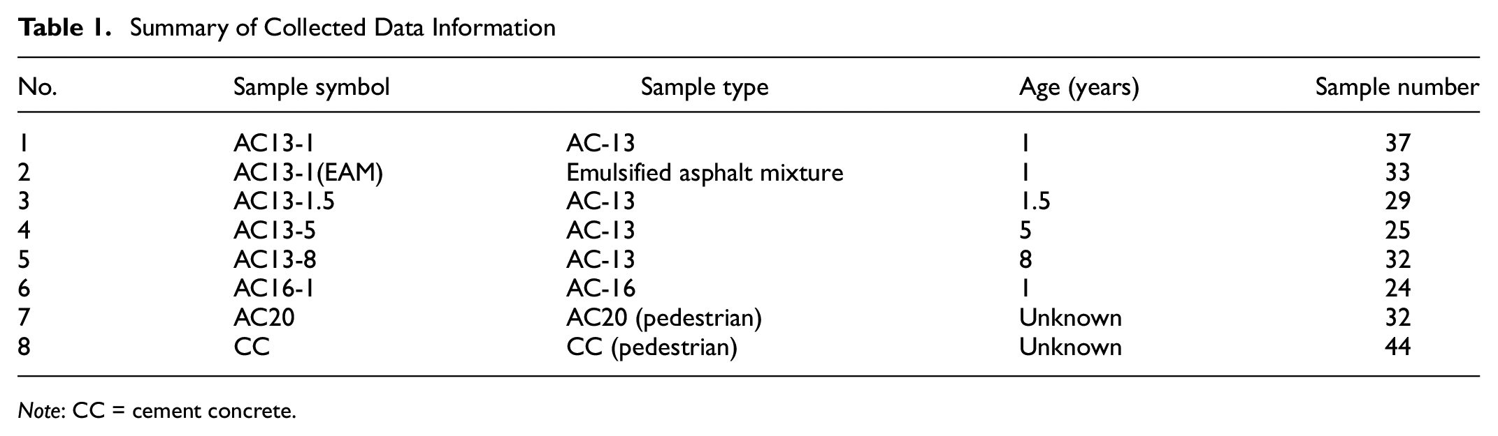
Note: CC = cement concrete.
In this study, a 3D scanner was used to capture high-resolution pavement surface data. The point spacing ranges between 0.015 and 0.1 mm. The measurement resolution varies from 0.001 to 0.5 mm, depending on the distance between the lens and the captured sample. Before collection, the scanner was first calibrated to identify the coordinates of the texture sample. Subsequently, the magnetic contrast Aid (FC-5) was sprayed uniformly on the pavement surface. All relative coordinates of the scanned texture were determined based on the triangulation principle. During the collection process, the scanner was moved around the target sample to capture the points on the pavement surface. Examples of the collected 3D point cloud data for the eight pavement surface textures and their corresponding grayscale images are presented in Figure 1.
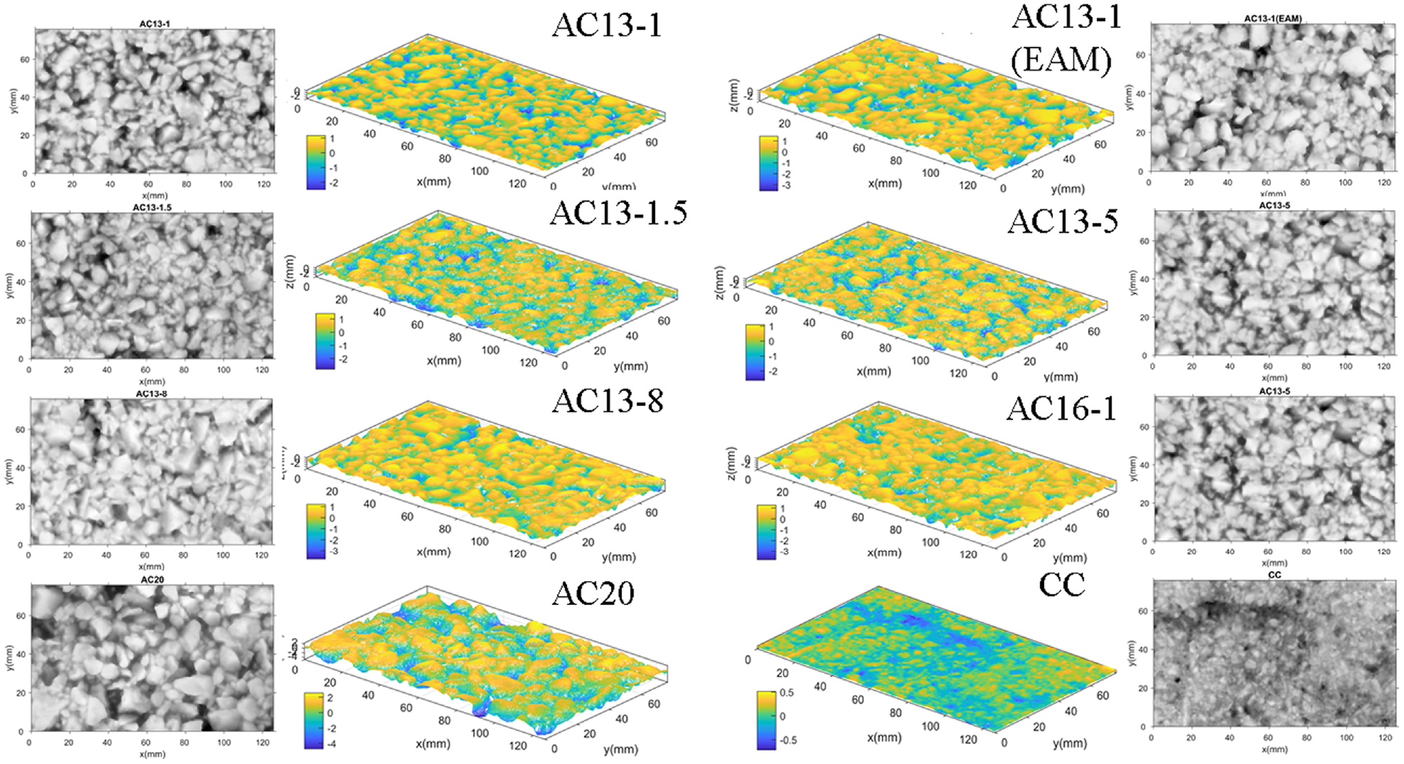
Visualization of the collected pavement surface textures.
Data Preprocessing
The collected raw data requires two preprocessing steps before model training, namely homogenization and planarization. Point cloud data were first homogenized by interpolation method with 0.5 mm point spacing ( 34 ). The reference plane was then adjusted according to the mean square regression plane. Elevation values of the final processed point cloud were transformed into a square matrix for classification training. Figure 2 illustrates the entire process of data preprocessing.
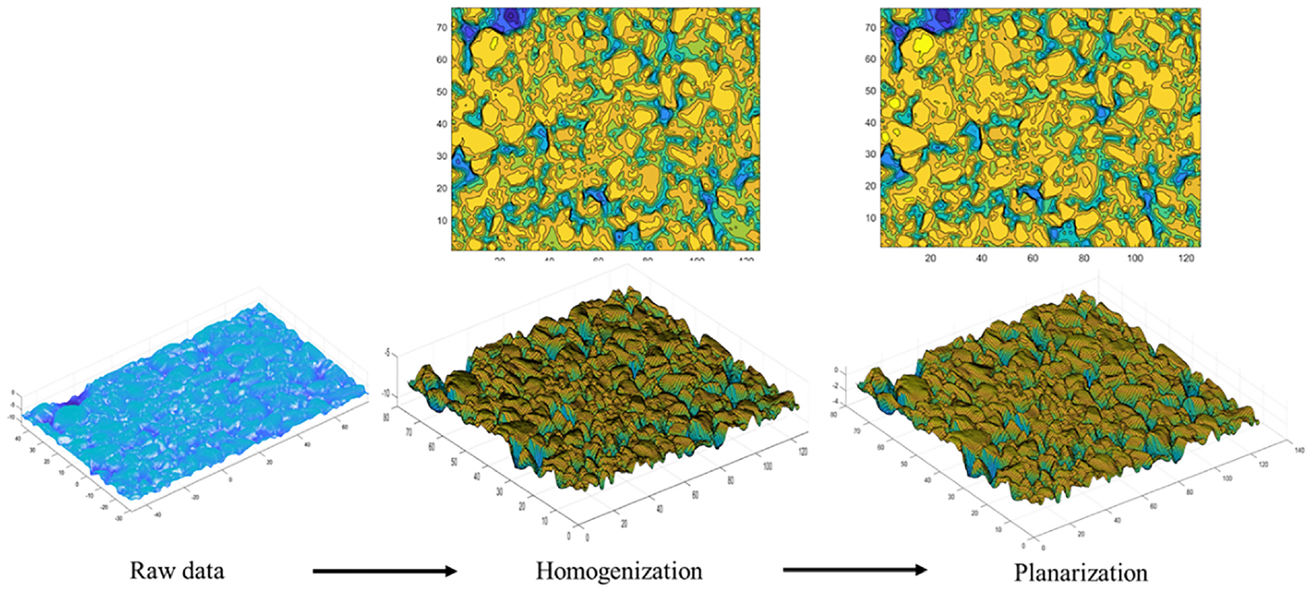
Schematic diagram of data preprocessing.
Data Annotation and Splitting
A reasonable model should balance both computational accuracy and computational efficiency, which are closely related to the size of the input samples. Considering that the maximum nominal particle size in the sample is 20 mm, the input sample size should be larger than 20 mm. On the other hand, a larger sample size would sacrifice computational efficiency and improve the requirement of dataset volume for training. In this study, the physical sample length of 32 mm × 32 mm is chosen as a balance of the contradiction ( 35 ). Considering that the point cloud data are homogenized with 0.5 mm point spacing, the input data matrix has a size of 65 × 65 accordingly.
To take full advantage of texture samples, a fixed 65 × 65 matrix with different angles and positions was randomly built into the samples to augment input samples, as shown in Figure 3. Original samples were split into two pieces to avoid the interference of datasets before data augmentation with a split ratio of 4:1 for the training-validation set and test set, respectively, which eliminates the overlapping of texture data.
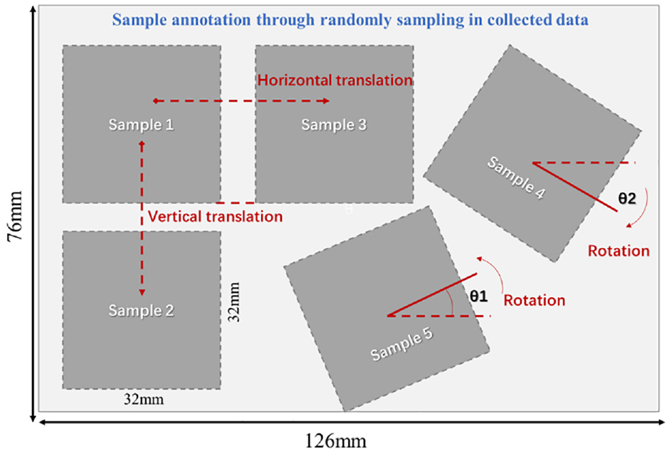
Input sample data annotation.
Methodology
This study investigated two representative machine learning methods to establish pavement classification models, namely the CNN and SVM. The advantage of the CNN is that the whole texture points can be used as the input data without preselecting the texture indicators, which avoids the loss of texture information. Meanwhile, the CNN shows good fault tolerance and powerful feature extraction and expression capabilities, which are qualities required for texture classification ( 36 – 38 ). For the SVM, as a typical traditional machine learning method, it does not make any assumptions about the distribution of the original data, which indicates that the SVM model has low requirements for data distribution. Since the texture distribution is random and irregular, the SVM is also a good choice for classification.
Convolution Neural Network
Architecture of the CNN
The CNN is a feed-forward neural network, which consists of an input layer, convolutional layers, activation layers, pooling layers, a full connection layer, and an output layer. Each neuron output of the network layers is locally connected to its input ( 39 ). A CNN model with 16 layers was built in this study for pavement surface texture classification. Figure 4 shows the CNN architecture.
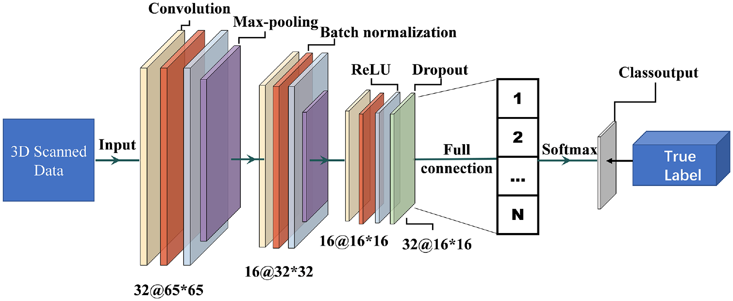
Convolutional neural network architecture.
The input layer serves as the entrance of the network for the preprocessed texture data, as aforementioned in the Data Preprocessing section, while the convolution layer is the key operation for feature extraction by taking the inner product of the input data and filters with defined weights. The nonlinear factors in the network are introduced via the activation layer, which boosts the capability of dealing with complex problems. To decrease the size of model parameters, the pooling layers are designed to further extract the main features. A fully connected layer is set before the output layer to integrate all weighted features into one representative feature, based on which the predicted labels are obtained and output via the output layer. To improve the computational accuracy, the network depth can be increased appropriately, which in turn leads to network overfitting and gradient dispersion issues ( 40 ). The dropout rate ( 41 ) and batch normalization operation ( 42 ) are then put forth. The networks are trained by adjusting the model parameters based on the gradient descent algorithm until the deviation between the predicted and real labels is within the allowance range, which indicates that the model is well-trained.
Considering that texture samples have various maximum nominal particle diameters, convolution kernels of three sizes are designed to capture the texture characteristics within different local receptive fields. It was proved that the model's training accuracy and test accuracy could reach a satisfying result. Table 2 lists the detailed dimensions of each layer and operation. The model was implemented using MATLAB and trained with a computer equipped with an Intel Core i7-8500U CPU, 8.00 GB RAM, and an NVIDIA GeForce MX 150 4 GB GPU.
Dimensions of Layers and Operations
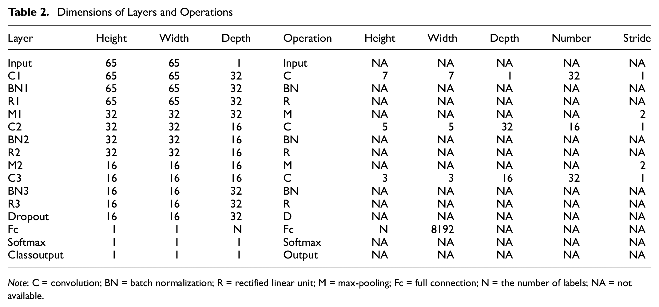
Note: C = convolution; BN = batch normalization; R = rectified linear unit; M = max-pooling; Fc = full connection; N = the number of labels; NA = not available.
Protocols of the CNN Model
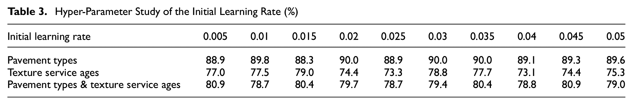
Before using the CNN model, it is necessary to determine the optimal parameters of the model. The hyper-parameter study of the initial learning rate, dropout, and gradient descent method was performed with 20 epochs based on the test accuracy. The batch size was set to 128. Early stopping was applied to select the model weights that obtained the best performance on the validation dataset during training. The validation dataset was not used to update the weights. The selected weights were then used for the following model training stage.
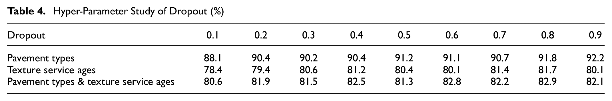
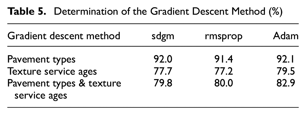
From Tables 3 and 4, it can be seen that the values of the learning rate and dropout settings do not have a significant effect on the accuracy when the learning rate and dropout are set between 0.005–0.05 and 0.1–0.9, respectively. Table 5 shows that the Adam algorithm has the best classification result. Comprehensively, the initial learning rate, dropout, and the gradient descent method are set to the best-performing 0.015, 0.8, and Adam, respectively.
Hyper-Parameter Study of the Initial Learning Rate (%)
Hyper-Parameter Study of Dropout (%)
Determination of the Gradient Descent Method (%)
SVM
The SVM, a binary classification model, implements classification by finding linear separators on the defined feature space. Note that it is challenging to directly classify texture service conditions based on whole texture samples with an excessive number of coordinate points. To reduce the data dimension, texture features that can distinguish samples are preselected manually. Then the extracted feature vectors are input into the SVM for training. Here the wavelet theory was used for feature extraction.
Feature Vector Extraction
Wavelet Theory
Wavelet theory can characterize features both in the time and frequency domains and has the capability of multi-resolution. Generally, wavelet theory has been widely used in signal and image processing. The basic idea of two-dimensional discrete wavelet decomposition is to perform low-pass and high-pass filtering from horizontal and vertical directions. The decomposition process is based on a set of shifted and dilated wavelet functions ψH, ψY, ψD, and scaling functions φ, which form an orthonormal basis for L2 (R2). For a two-dimensional M×N matrix f(x,y), the discrete wavelet transform is performed as follows:
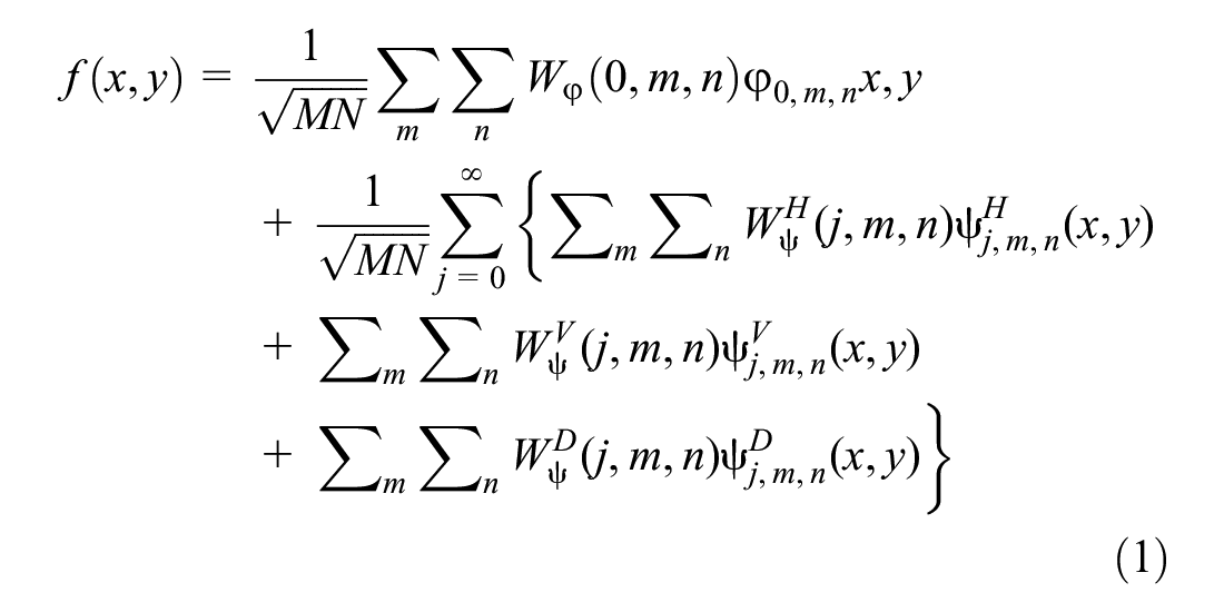
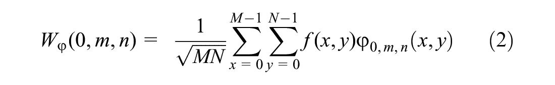
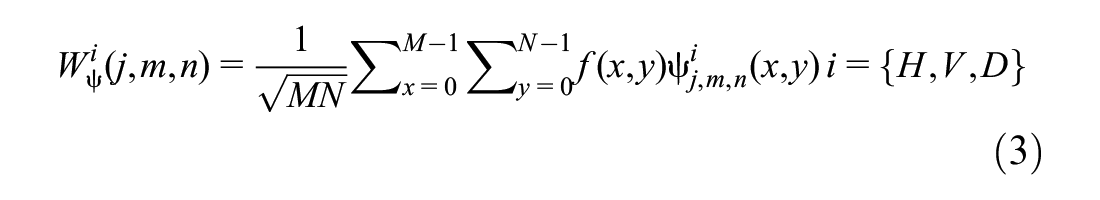


where
Wavelet Decomposition
Daubechies (Db) wavelets are widely used to process signals and images at various scales because of their orthogonality and compact support, which are ideal properties for iterative decomposition. The most common mother wavelet in transportation-related applications is the Db3 mother wavelet. Favorable results have been achieved by using this mother wavelet to analyze the surface texture ( 43 , 44 ), roughness ( 45 ), and vehicle–pavement interaction ( 46 ). Therefore, Db3 was chosen as the mother wavelet in this study to decompose the texture data. Since the minimum interval of texture is 0.5 mm and the upper limit of input texture wavelength is 32 mm, six-layer wavelet decomposition was used. The decomposition diagram is shown in Figure 5.
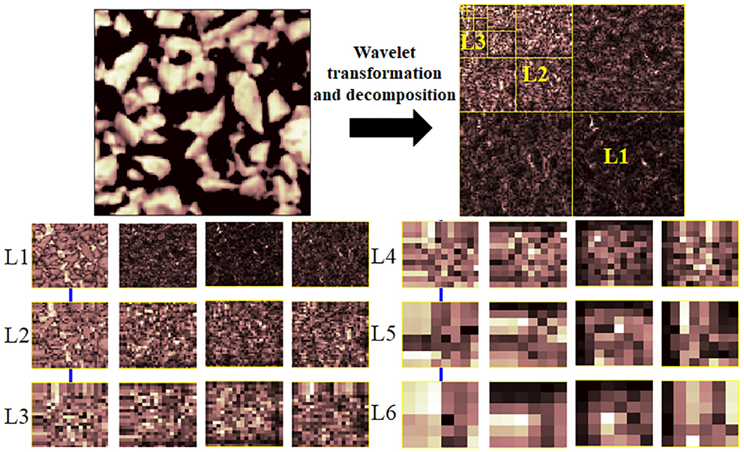
Wavelet decomposition diagram of the pavement surface texture.
Feature Extraction
According to the coefficients decomposed by the wavelet, the feature indexes at each scale can be extracted, and the feature vector can be constructed by transforming the coefficient. Commonly used indicators are the mean (M), entropy (EN), energy (E), and standard deviation (S) ( 47 ). Here they are collectively referred to as EEMSD:

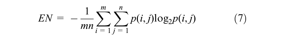
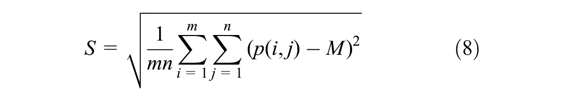

where p(i,j) is the amplitude of the decomposed m×n subband at (i, j).
SVM Classification
Based on the preselected features obtained by wavelet decomposition, the further classification of the service conditions of the pavement surface texture can be achieved by the SVM. The texture classification process used a multi-class SVM (
48
) based on the standard one-versus-one approach to reduce the single multi-class problem into multiple binary classification problems. For each texture sample, the extracted feature vectors
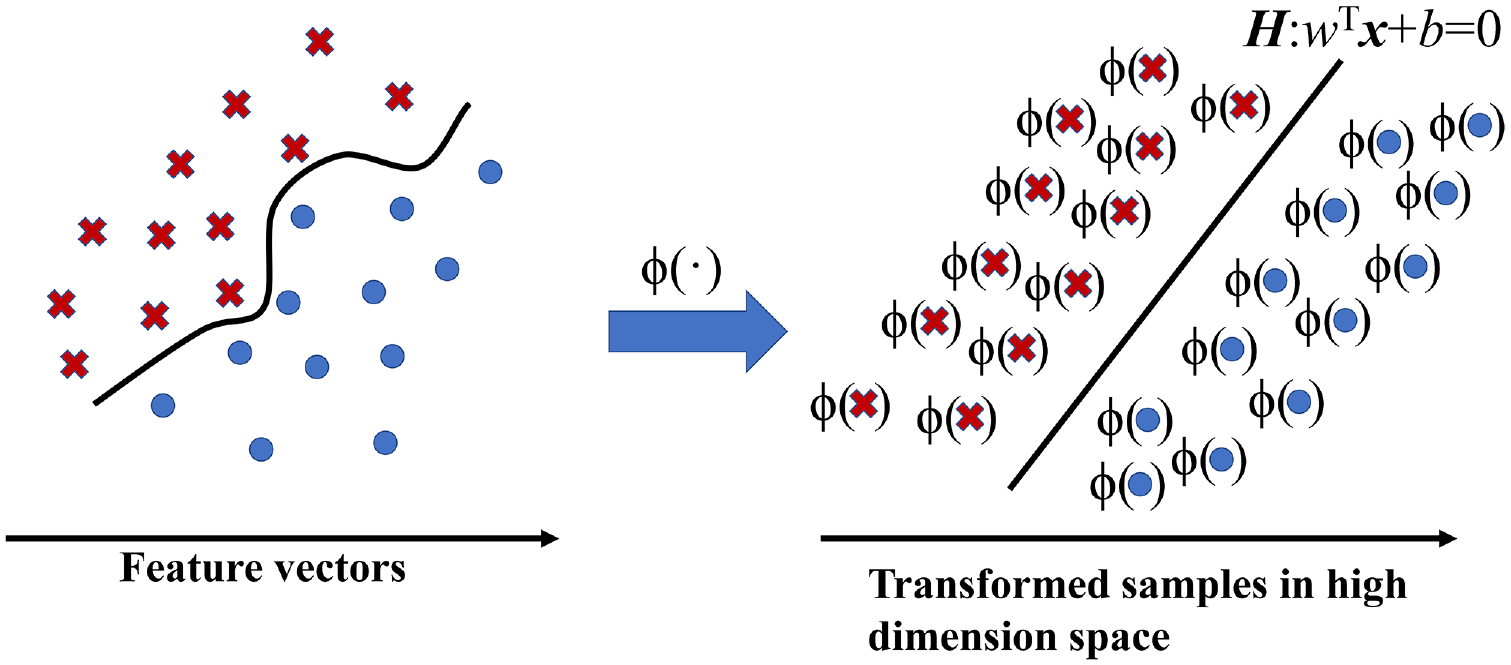
Transformation using kernel functions.
In this study, a quadratic kernel function has been chosen to achieve the best accuracy when compared with linear, cubic, and Gaussian kernel functions. The SVM adopted a cross-validation method when performing classification training in this study.
Experiment Design
Considering the stochastic complexity of the surface texture distribution, 10,000 augmented samples were used for each pavement to fully cover the collected texture information. The large input dataset size also reduces the number of training epochs accordingly. Specifically, 2000 of them were used to test the training results and 7200 samples were subjected to the model training, while the remaining 800 samples were used for the validation. Pavement types and texture service ages were used as classification objects to discuss the classification performance of the CNN and SVM. For further comparative analysis of the impact of increased categories on the classification accuracy, the CNN and SVM were also used to train a universal model for the combined classification objects, including pavement type (AC13, AC13(EAM), AC16, AC20, and CC) and texture service age (1, 1.5, 5, and 8) for AC13. For convenience, the combined classification case is referred to as both pavement type and texture service age.
Metrics
Confusion Matrix
The confusion matrix was used to visualize the classification results with combinations of predicted and actual values. As shown in Figure 7, in a confusion matrix M = (
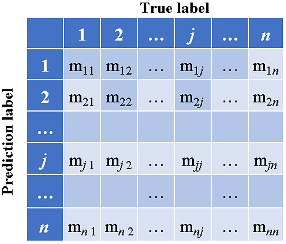
Schematic of the confusion table.
In addition, the precision, recall, and accuracy for the classification of multi-class pavement surface service conditions were calculated:


where Precisionj is the proportion of prediction results where the actual value is also type j, Recallj indicates the proportion of samples with the actual value j that are accurately predicted to be type j, and Accuracy represents the comprehensive classification accuracy of the model.
Receiver Operating Characteristic
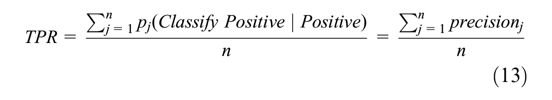
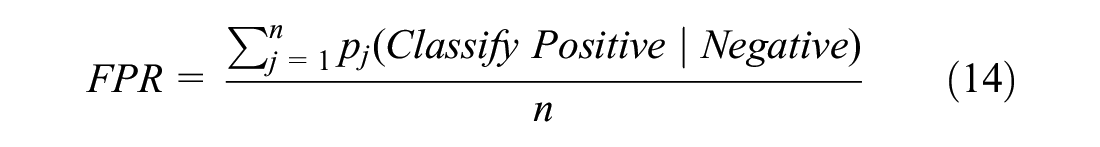
To compare the relative performance of the trained classifier based on the CNN and SVM and validate whether the classifiers perform better than random guessing, receiver operating characteristic (ROC) analysis, which measures the classifier by examining the trade-off between the successful identification of positive samples and the misdetection of negative samples, was introduced in this study ( 49 ). In the ROC space, the true positive rate, TPR, and false positive rate, FPR, of a classifier are plotted on the Y- and X-axes, respectively. Considering that the involved classifications are multi-class tasks and the sample labels are uniformly distributed, the average ROC across all categories in the classification case was calculated to evaluate the model performance generally, as shown in Figure 8. Specifically, let p(P∣I) be the probability that instance I is estimated to be positive on a test set. The TPR and FPR of a classifier are as follows:
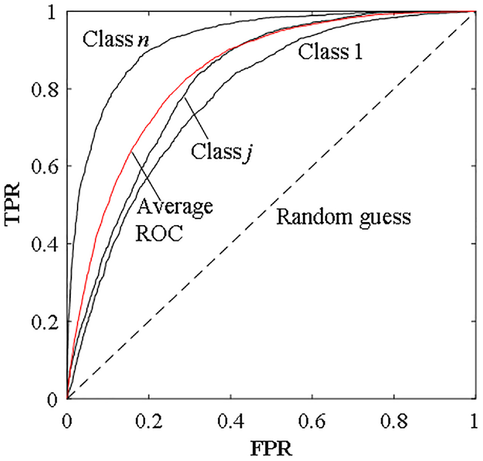
Schematic diagram of the receiver operating characteristic (ROC).
These two statistics vary together as the threshold of the classifier is altered between its extremes, and then the resulting ROC curve is drawn. For orientation, the point (0, 0) in the ROC space corresponds to an extremely conservative classifier, which yields no true positive. Similarly, the point (1, 1) represents a classifier that declares every sample to be positive. Since the point (0, 1) corresponds to the ideal classifier in which both positive and negative samples are issued perfectly, points closer to the upper-left corner of ROC space are generally better classifiers. In contrast, a random classifier produces points that reside along the diagonal line connecting the bottom-left to the upper-right corner of the ROC graph.
Results and Discussion
Classification Model of the Pavement Type
The loss curves for the CNN during the training process are shown in Figure 9. It can be seen that the loss curves for the training and validation dataset are close and show a continuously downward trend. Notably, validation samples are different from training samples yet partially contain textures overlapped with the training samples induced by the sample data annotation method. In this regard, overfitting during the training process is diagnosed as not obvious. Meanwhile, the loss for both training and validation datasets decreases continuously with iterations and shows a slow downward trend after about 25 epochs. Based on the trade-off between computation load and efficiency, the 30 epochs were finally adopted. Table 6 summarizes the precision, recall, and accuracy for different pavement types using the CNN and SVM.
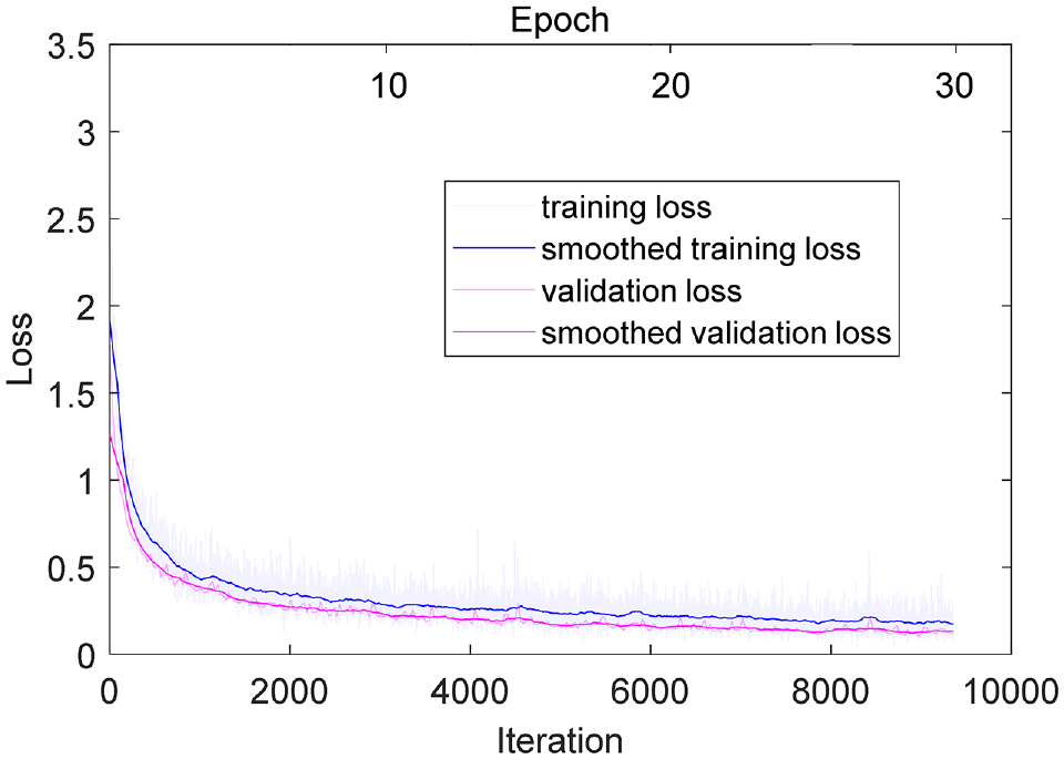
The loss curves during the convolutional neural network training process for classification of pavement types.
Model Merits of Classification of Pavement Types (%)
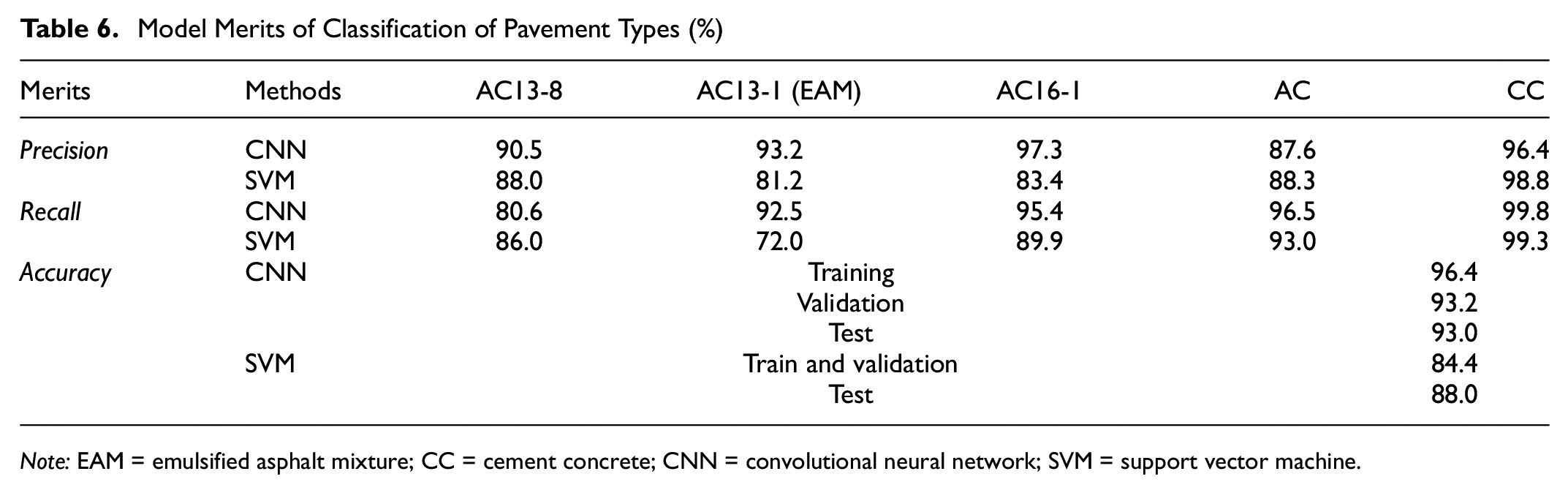
Note: EAM = emulsified asphalt mixture; CC = cement concrete; CNN = convolutional neural network; SVM = support vector machine.
The trained CNN classification model has a satisfying outcome, as it can be seen that the training, validation, and test accuracy all exceed 90%. It demonstrates that the CNN model could extract features effectively from randomly distributed textures. As for the SVM, it shows relatively low accuracy, as it is observed that the accuracy results are limited between 80% and 90%. Concerning the average precision and recall for different pavement types, it can be found that the overall performance of the CNN classification model for different textures follows the sequence of CC > AC16-1 > AC13-1(EAM) > AC20 > AC13-8 (Figure 10).
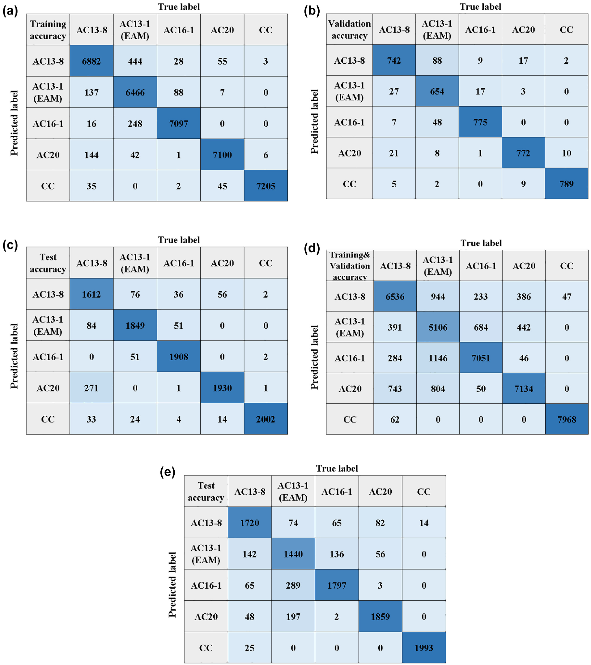
Confusion matrixes of the convolutional neural network (CNN) and support vector machine (SVM) for classification of pavement types: (a) CNN training set, (b) CNN validation set, (c) CNN test set, (d) SVM training and validation set, and (e) SVM test set.
The misclassification of the SVM is distributed among types AC13-8, AC13-1 (EAM), AC16-1, and AC20. It may be attributed to the loss of important data information when manually extracting features after wavelet decomposition. In addition, the differentiation for type CC is still better than others, which may be because type CC has clearly distinguishing features. In conclusion, for those with distinct features, both the CNN and SVM could obtain the desired classification results. However, the CNN outperforms the SVM when it comes to categorizing samples with indistinct features.
Classification Model of the Texture Service Age
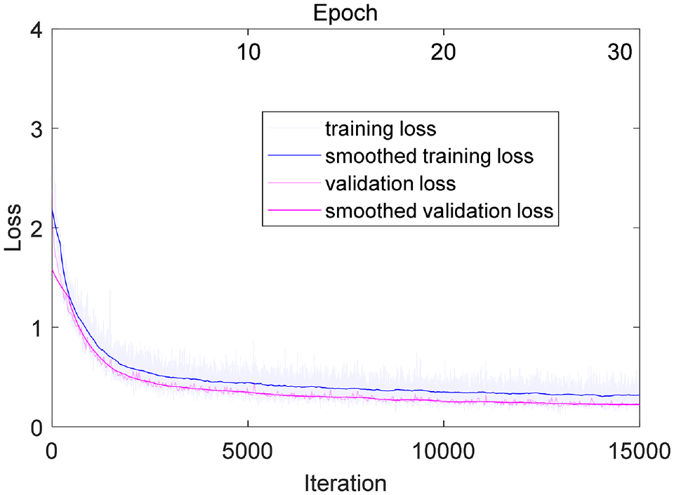
Concerning the adequacy of the texture data source and its diversity of service ages, AC13 was adopted as an example to explore the classification performance of the CNN and SVM for texture service ages with the same aggregate gradation. The loss curves for the CNN during the training process are shown in Figure 11. Table 7 lists the classification results of the CNN and SVM. It can be seen that the SVM fails in classifying the years of service. On the other hand, the CNN could still achieve satisfactory results for service age classification, indicating good capability of dealing with complex random data with no distinct features. Compared to the Classification Model of the Pavement Type section, the accuracy of the CNN model in classifying the texture service ages decreases, which is in line with our general perception. It is because the variability of the same type of pavement caused by the service age is lower than that of aggregate gradation. From Table 7, it can be found that the overall performance of the CNN for classifying the four types of pavements is in the order of AC13-1 > AC13-8 ≈ AC13-1.5 > AC13-5.
Loss curves during the convolutional neural network training process for the classification of service ages.
Model Merits of Classification of Texture Service Age (%)
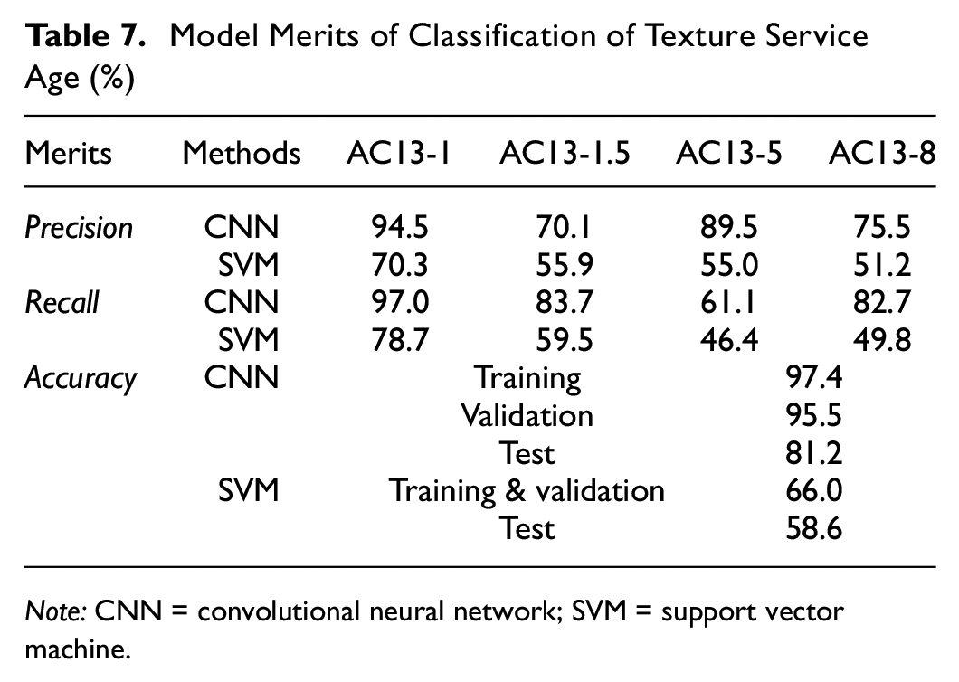
Note: CNN = convolutional neural network; SVM = support vector machine.
By observing the distribution of misclassified samples in Figure 12, it can be found that the main misclassification was that some type AC13-5 samples are misclassified as types AC13-8 and AC13-1.5, which may be because texture samples from different locations had undergone varying degrees of abrasion. Besides, there is a small amount of mutual misclassification between types AC13-1.5 and type AC13-8, as some areas with similar features inevitably exist between the same pavement surface texture. However, most samples could be well classified using the CNN model.
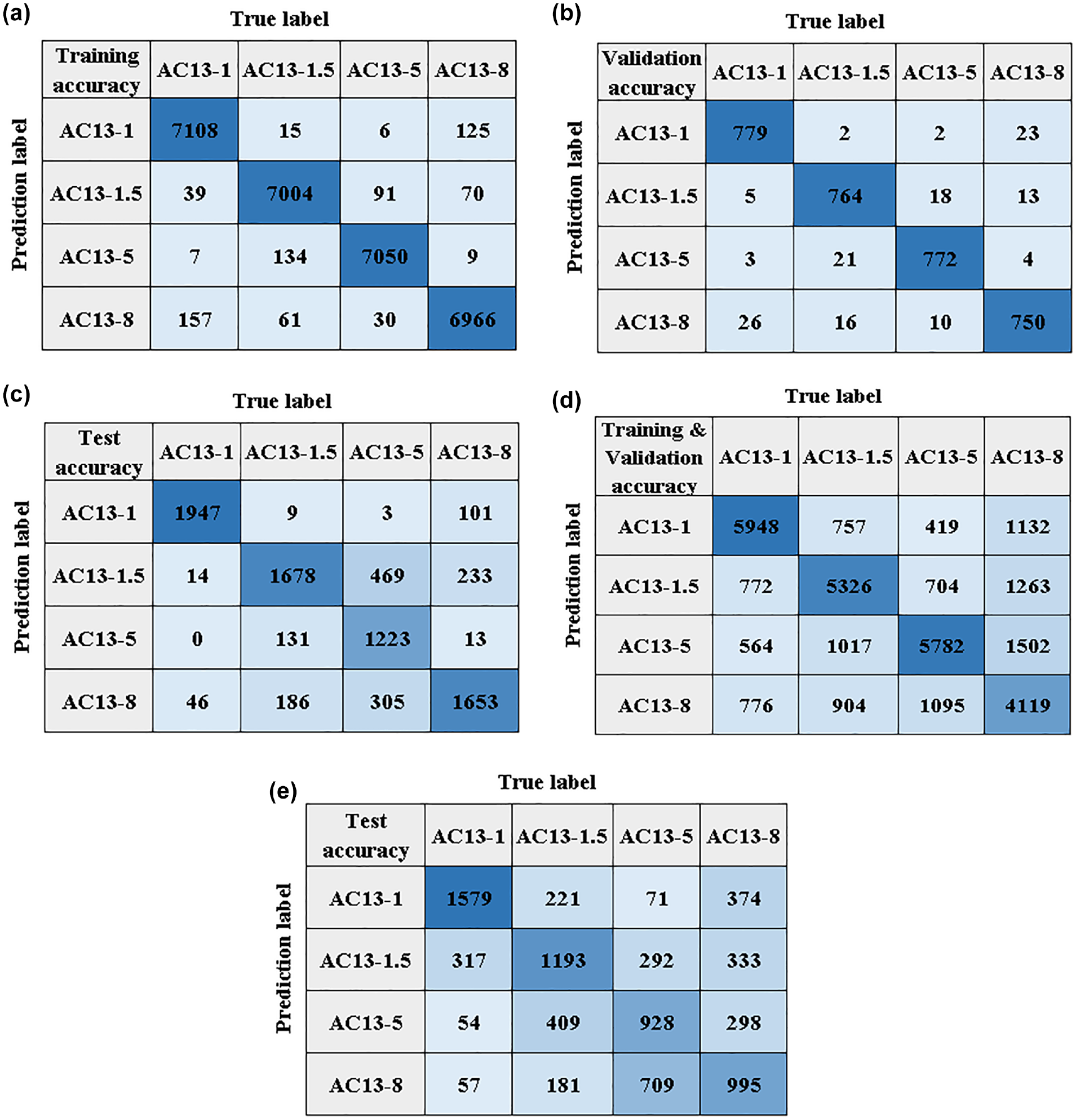
Confusion matrixes of the convolutional neural network (CNN) and support vector machine (SVM) for classification of service ages: (a) CNN training set, (b) CNN validation set, (c) CNN test set, (d) SVM training and validation set, and (e) SVM test set.
Classification Model of Both Pavement Type and Service Age
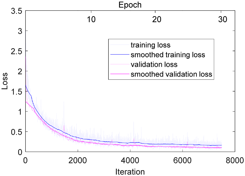
The loss curves for the CNN during the training process are shown in Figure 13. Table 8 lists the classification results of the CNN and SVM on the service state of the eight textures. It can be seen that the classification accuracy of the SVM method for both the training and validation dataset and the test dataset is very low. In contrast, the CNN has a comprehensive accuracy rate of 83.8%. Concerning the average precision and recall for different texture types, the overall performance of the CNN classification model follows the sequence of CC > AC16-1 > AC20 > AC13-1 (EAM) ≈ AC13-1 > AC13-5 > AC13-8 > AC13-1.5.
Loss curves during the convolutional neural network training process for classification of both pavement type and texture service age.
Model Merits of Classification of Both Pavement Type and Texture Service Age (%)
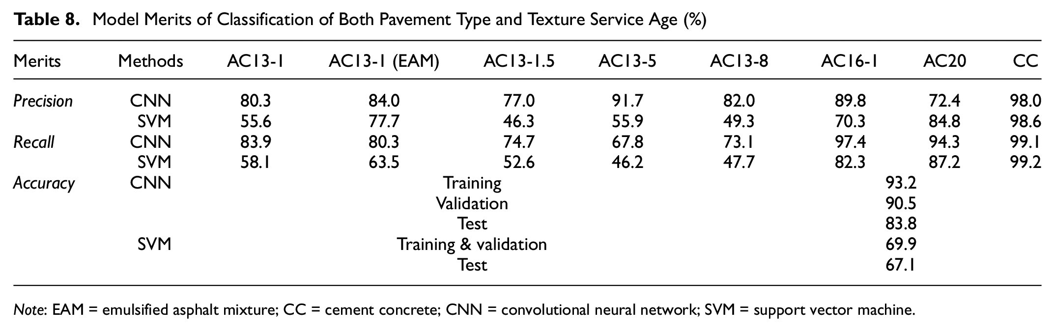
Note: EAM = emulsified asphalt mixture; CC = cement concrete; CNN = convolutional neural network; SVM = support vector machine.
By comparing Tables 6–8, it can be seen that the classification accuracy of types AC13-8, AC13-1 (EAM), AC16-1, AC13-1, AC13-1.5, AC20, and CC, which have apparent features, are all reduced. It can be inferred that when the number of classification categories increases, the feature extraction process takes all of the characteristics contained in each type into account simultaneously, leading to a universal decrease in classification accuracy. Based on this, the necessity of classifying various types of pavement surface textures before analyzing the performance of pavement surface textures is indirectly confirmed. However, it is worth mentioning that the classification results of type AC13-5 have been improved, as shown in Figure 14. This may be because the increase of the texture category promotes the further extraction of effective features from type AC13-5 samples whose features are not evident. Therefore, when classifying texture service conditions with significant differences, reducing classification categories can result in obtaining a better classification performance. On the other hand, when classifying texture service conditions with few differences, increasing the categories of input samples helps to improve the classification accuracy.
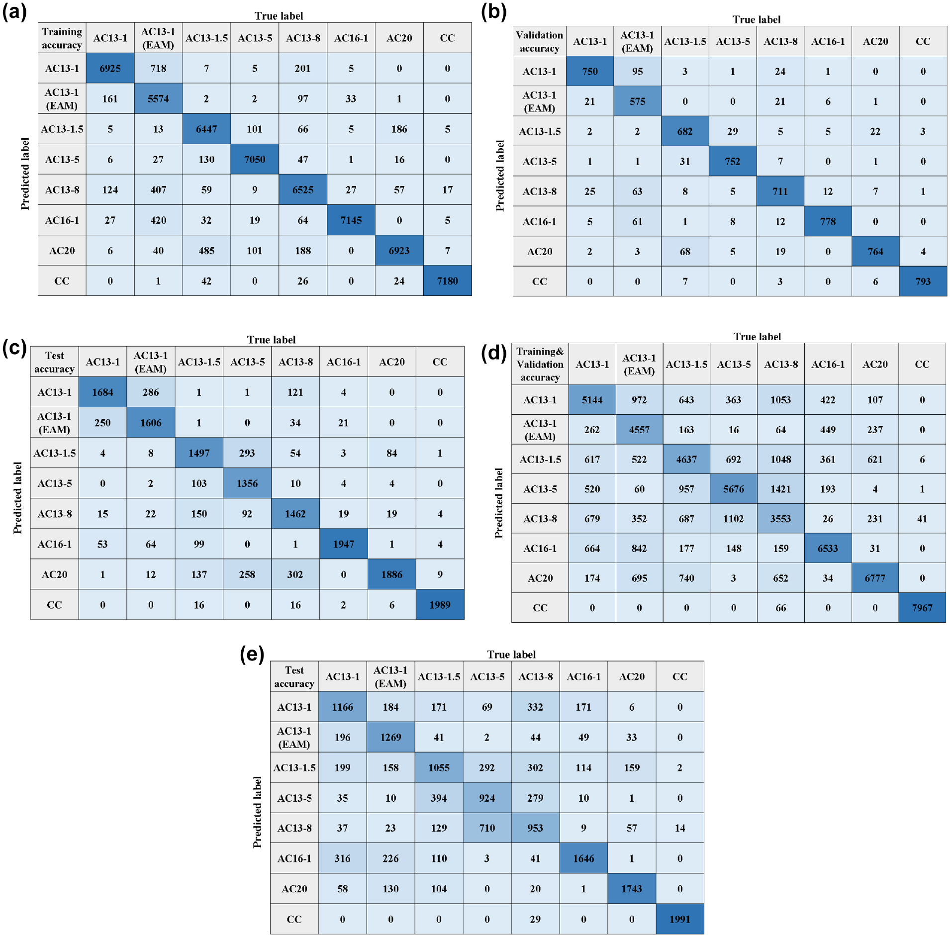
Confusion matrixes of the convolutional neural network (CNN) for classification of both pavement type and texture service age: (a) CNN training set, (b) CNN validation set, (c) CNN test set, (d) support vector machine (SVM) training and validation set, and (e) SVM test set.
Performance Evaluation Between the CNN and SVM Methods
Figure 15 shows the ROC of the CNN and SVM models for the three classification cases based on the test datasets. It can be seen that the designed CNN classifiers are discrete-valued output mapped to a single point in the ROC graph because the involved parameters were trained to find the only one optimal solution in the self-supervised learning process, whereas the SVM based on the standard one-versus-one approach produces numeric-valued outputs forming a piecewise linear curve by varying the threshold that determines whether a new sample belongs to the target class. Obviously, the ROC curves of the SVM are above the random guessing line, which indicates that the classification results of the SVM classifiers are not achieved only by chance. In addition, it should be mentioned that the one-versus-one calculation principle of the SVM caused skewed class distribution issues. The slope of the iso-performance line for best-performing SVM model adoption was then adjusted from 1 to 4 (type), 3 (age), and 7 (type and age), respectively according to the category number ( 50 ). The optimum SVM classifiers are marked in Figure 15. Consistent with the results of the confusion matrix, the SVM and CNN perform best in the type classification case, followed by the classification case of both type and age. The performance of age classification is the worst. Moreover, compared to the SVM classifiers for each case, the ROCs of the CNN classifiers are closer to the upper-left corner in the ROC space, proving a superior performance of the CNN compared with the SVM in the texture type and age identification tasks.
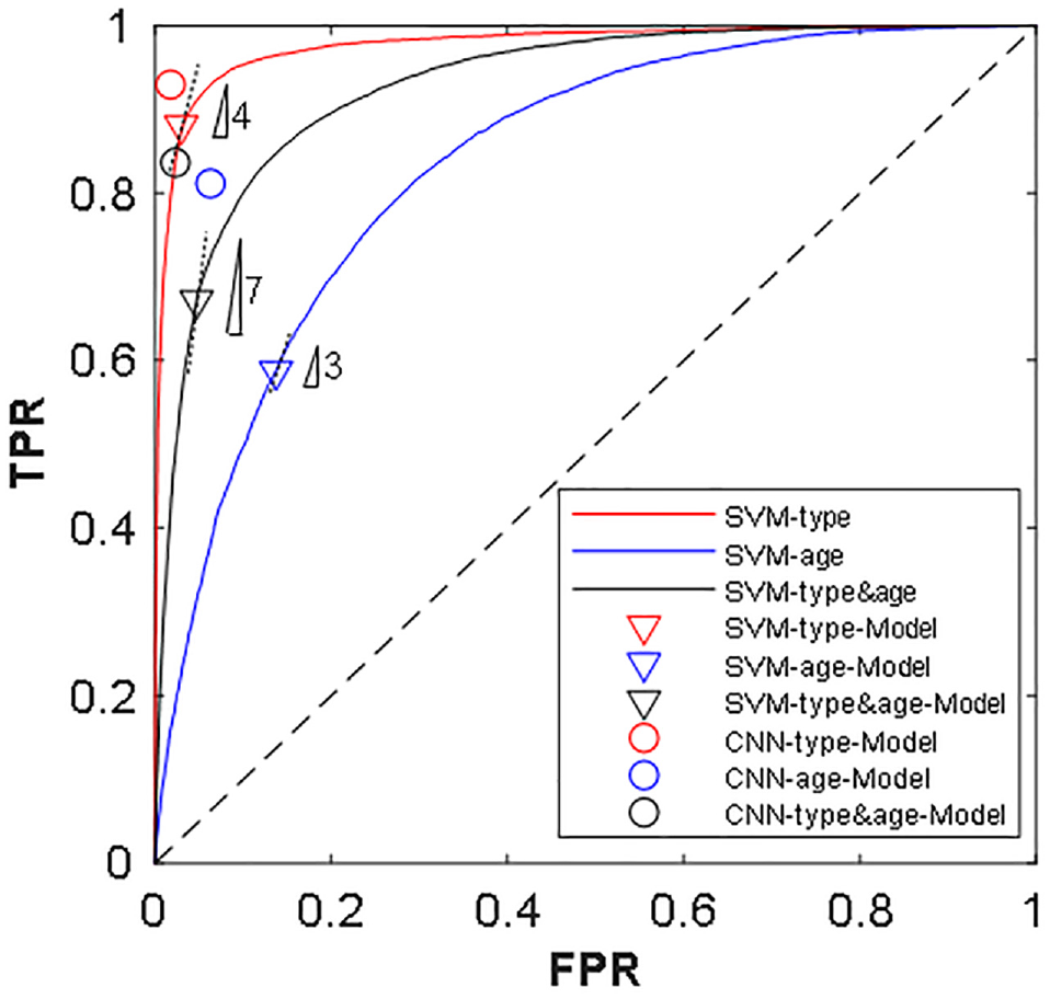
Receiver operating characteristic of the convolutional neural network (CNN) and support vector machine (SVM) models.
Conclusions
The classification of the service condition of pavement surface textures is an essential premise for the evaluation of texture-related pavement performance in pavement management systems. However, there is still a lack of effective methods for classifying the service conditions of common pavement surface textures with respect to pavement types and texture service ages. Considering the unclear recognition of texture features induced by the random irregular distributions, the CNN was adopted to explore an automated service condition classification model based on pavement surface texture. Three classification cases, case 1: pavement type classification, case 2: texture service age classification, and case 3: the classification of texture service conditions involved in the above two cases, were studied consecutively. To illustrate the advantages of the CNN models, the typical machine learning method, namely the SVM, was used simultaneously for the same classification cases. Considering the limitations of this study, the results show promising outcomes.
(1) The proposed CNN model achieves favorable classification accuracies of 93.0%, 81.1%, and 83.8% in the three cases, respectively.
(2) For the classification of pavement types with distinct texture features, both the CNN and SVM achieve good classification results of 93.0% and 88.0%, respectively. However, for the classification of service ages, the CNN shows good classification results of 81.2%, while the SVM fails with an accuracy of 58.6%.
(3) For the classification of pavement types with distinct texture features, such as AC13-8, AC13-1 (EAM), AC16-1, AC13-1, AC13-1.5, AC20, and CC, the increased classification categories tend to act as interference information, thus reducing the classification accuracy. However, for the classification of service ages with indistinct texture features (AC13-5), the increased classification categories could guide a further extraction of texture features, therefore increasing the classification accuracy.
(4) The ROC of both the SVM and CNN are above the random guessing line in the ROC space, proving that the classification results of the classifiers are not achieved only by chance. Compared to the SVM classifiers for each case, the ROCs of the CNN classifiers are closer to the upper-left corner.
Limitations and Future Work
It should be mentioned that the models in this study were trained under a limited variety of texture service conditions. Meanwhile, the label of texture ages is a rough mark without comprehensively considering the actual texture wearing status. Therefore, with respect to the practical application in pavement management systems, the automatic identification models for texture data still deserve further investigation and this study is supposed to serve as a foundational exploration. Based on this initial study, future work may include the following aspects.
(1) The interpretability of the texture feature latent extracted by machine learning methods should be studied further to improve the CNN architectures.
(2) The practical performance of texture samples with a finer or coarser grid should be studied further in the future to achieve a balance between classification accuracy and efficiency.
(3) A standard texture database should be established and expanded by involving factors beyond pavement type and surface age, such as aggregate type, shape, surface texture, and gradation, as well as surface condition and skid resistance measurement methods to further enhance the generality of the CNN models. Once new texture samples are input into the models, the texture condition benchmarked with the standard texture database could be obtained.
(4) Methodologies to embed the well-trained CNN model into the follow-up process of texture performance evaluation and maintenance decision-making still deserves further investigation.
Footnotes
Acknowledgements
We gratefully acknowledge the highway engineering laboratories at Dalian University of Technology.
Author Contributions
The authors confirm their contribution to the paper as follows: study conception and design: J. Lu, B. Pan, Q. Liu; data collection: J. Lu; analysis and interpretation of results: J. Lu; draft manuscript preparation: J. Lu., B. Pan, Q. Liu, P. Liu, M. Oeser. All authors reviewed the results and approved the final version of the manuscript.
Declaration of Conflicting Interests
The author(s) declared no potential conflicts of interest with respect to the research, authorship, and/or publication of this article.
Funding
The author(s) received no financial support for the research, authorship, and/or publication of this article.
Data Accessibility Statement
Some or all data, models, or codes that support the findings of this study are available from the corresponding author on reasonable request.