Use of Machine Learning for Automated Classification of Sand Type

Abstract

This study demonstrates the feasibility of utilizing machine learning (ML) for routine identification of sand particles. Identifying different types of sand is necessary for various geotechnical exploration projects because understanding the specific sand type plays an important role in estimating the physical and mechanical properties of the soil. To accomplish this, dynamic image analysis was employed to generate a substantial volume of sand particle images. Individual size and shape descriptors were automatically extracted from each particle image. The analysis involved use of 40,000 binary particle images representing 20 different sand types, and a corresponding six size and four shape descriptors for each particle (400,000 parameters). Six ML models were trained and tested. The work demonstrates that using size and shape features the models efficiently identified up to 49% of individual sand particles. However, when clusters of particles were considered in conjunction with a voting algorithm, classification accuracy significantly improved to 90%. Among the ML models studied, neural networks performed the best, while decision tree exhibited the lowest accuracy. Finally, the use of size consistently outperformed shape as a classification parameter but combining size and shape parameters yielded superior results across all sands and classifiers. These findings suggest that ML holds much promise for automating sand classification using ordinary images.

Keywords

data and data science machine learning (artificial intelligence)geology and geoenvironmental engineering engineering geology geotechnical engineering soil characteristics soil classification

The identification and categorization of soils not only play a vital role in the fields of geotechnical, geological, and hydrological engineering but also contribute to well-informed decision-making for construction, agriculture, and environmental activities ( 1 , 2 ). Traditionally, the sieve analysis method has been the conventional means of ascertaining the distribution of sand particle sizes within geotechnical engineering. However, this method is labor-intensive and time-consuming, and provides results of limited accuracy, especially for particles smaller than 300 µm ( 3 ). Additionally, the process becomes more intricate when attempting to characterize particle shapes. The classic method for shape classification involves the utilization of the Krumbein-Sloss chart, which relies on visually comparing particles with reference images, making the process both cumbersome and susceptible to subjectivity ( 4 , 5 ).

Supervised machine learning (ML) algorithms employ an automatic inductive approach to recognize patterns within data and establish connections between these patterns and their corresponding labels. Inductive reasoning involves drawing general conclusions from specific observations or examples. In the context of supervised ML, the term “inductive” signifies that these algorithms learn from specific labeled examples provided in the training data. They generalize patterns and relationships from the observed data to make predictions or classifications on new, unseen data. In simpler terms, the inductive approach of supervised ML involves learning from specific instances to make broader generalizations about how new, similar instances should be categorized or predicted. Once these relationships are learned, they can be applied to similar data to assign labels to new data points. This technique has been introduced for the automated identification and classification of mineral and volcanic ash particles and the spatial prediction of shallow landslides ( 6 – 8 ). However, most of these studies focused on large area scene analysis, such as geographic maps or plant leaves, which means it would not be suitable for the classification of sand type ( 9 , 10 ). None of these studies employed images where individual particles are visible. In addition, in some cases these studies employed complex stereo-images ( 11 ).

Dynamic image analysis (DIA) has been utilized for capturing images of individual particles, ranging in quantity from 1,000 to 1,000,000 particles ( 3 ). Recent advancements in image segmentation hold the promise of enabling the identification of individual particles within a standard sand image captured by a camera or a soil probe, such as a vision cone ( 12 ). However, DIA operates by capturing individual images of a moving specimen, creating a substantial collection of separate particle images. This obviates the need for segmenting the region of interest, resulting in a sizable image dataset suitable for statistical analysis and application in computer-vision-based soil classification. Moreover, DIA furnishes engineering descriptors for size and shape that can effectively represent sand characteristics across various scales ( 13 ). Lastly, a pre-trained ML classifier can produce identification results for a new specimen by utilizing the same class of image features used during training.

This research paper delves into the application of ML methods in the realm of sand classification. One of the primary goals of this study is to investigate the precision and efficiency of categorizing sand particles using various ML classifiers, all while utilizing engineering size and shape descriptors. This approach enables the accurate classification of individual sand particles to a satisfactory degree. Prior studies by the authors first involved the use of size and shape descriptors as features in ML, and identified which features are independent of each other ( 13 ). This first step was carried out using six sands. Next, the authors explored using seven different ML algorithms for classification of nine sands ( 14 ). In this work, we employ shape and size descriptors as features and vastly increase the difficulty of the classification task by extending the sands being classified to 20 using the six best-performing classifiers. In prior research, it was established that ML techniques, specifically neural networks (NN), could effectively identify 75% of sand particles by relying on size and shape descriptors across nine distinct sand types ( 14 ). The current study aims to evaluate the effectiveness of ML-based sand classification in tackling a considerably more intricate classification task. To accomplish this, a dataset featuring 20 distinct sand types was compiled and employed to train six distinct ML models. The analysis was conducted using 2,000 binary particle images for each sand type, which were obtained through DIA (i.e., images were black and white with no grayscale). The work demonstrates that ML-based classification of sand can be carried out swiftly, non-destructively, and precisely, at levels consistent with what can be expected from manual classification by a trained engineering geologist.

ML thus has the potential to alleviate the workload of geologists and engineers while enhancing accuracy by automating tasks that would otherwise be impractical because of the extensive time and effort required to process the vast amount of information.

Features Used for Sand Classification

Sand particles can be characterized as numerical values within ML models. These values must correspond to distinctive features that enable differentiation of various objects. Desirable features must be informative, discriminating, and independent, to permit effective analyses in ML models.

Engineering size and shape descriptors have long been used for particle classification ( 15 ). However, their use has been limited by the difficulty and labor-intensive nature involved in acquiring them manually. In recent years, micro-computed tomography, and especially DIA, have made acquiring this information feasible for large datasets.

DIA offers the opportunity of providing many size and shape features that can be used for classification with ML. The method employs a high-frame-rate camera combined with a pulsed laser to image millions of individual particles in a short time ( 3 ). DIA feeds specimens into a hopper that disperses particles to the imaging unit at a constant rate. A vibrating tray is used to help separate the particles (Figure 1). Particles fall through a 50 cm-long shaft into the imaging plane. 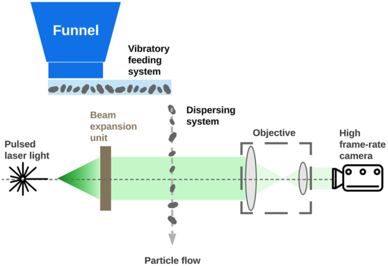As particles travel through the imaging plane, particle shapes are captured at a frame rate of up to 175 frames per second with a 4-megapixel ( $2, 336 \times 1, 728$ ) resolution. A pulsed laser is used for illumination which helps freeze particles and eliminate motion blur, but at the expense of causing the images to become binary (i.e., black and white). Next, the DIA software segments individual particle images. Finally, the system software computes a variety of shape and size descriptors that correspond to each captured image. The resulting particle image resolution is 4 µm/pixel, which limits this type of analysis to particles larger than 200 µm, since 200 µm would represent a particle diameter of 50 pixels, the minimum resolution, in the authors’ opinion, that is necessary for meaningful particle analysis.

Figure 1.

Schematic of dynamic image analysis device.

Commonly used size descriptors include equivalent projected circle (EQPC) diameter (d_e), maximum and minimum Feret diameter (d_Fmax and d_Fmin), maximum inscribed circle and minimum circumscribed circle diameters (d_ins and d_cir) and perimeter equivalent circle diameter (PED). These size descriptors can measure dimensions of irregular particles in multiple manners (Figure 2). Similarly, shape descriptors are able to capture global and intermediate scales of particle morphology. Four independent shape descriptors were identified by Li and Iskander, to represent: 1) proportion of axis (aspect ratio [AR]), 2) convexity (Cx), 3) smoothness of the perimeter (sphericity [S]), and 4) roundness of corners (Wadell roundness [R]) ( 13 ). In general, the values of shape descriptors range from 0.0 to 1.0, corresponding from an infinitely irregular particle to a perfect circle, respectively.

Figure 2.

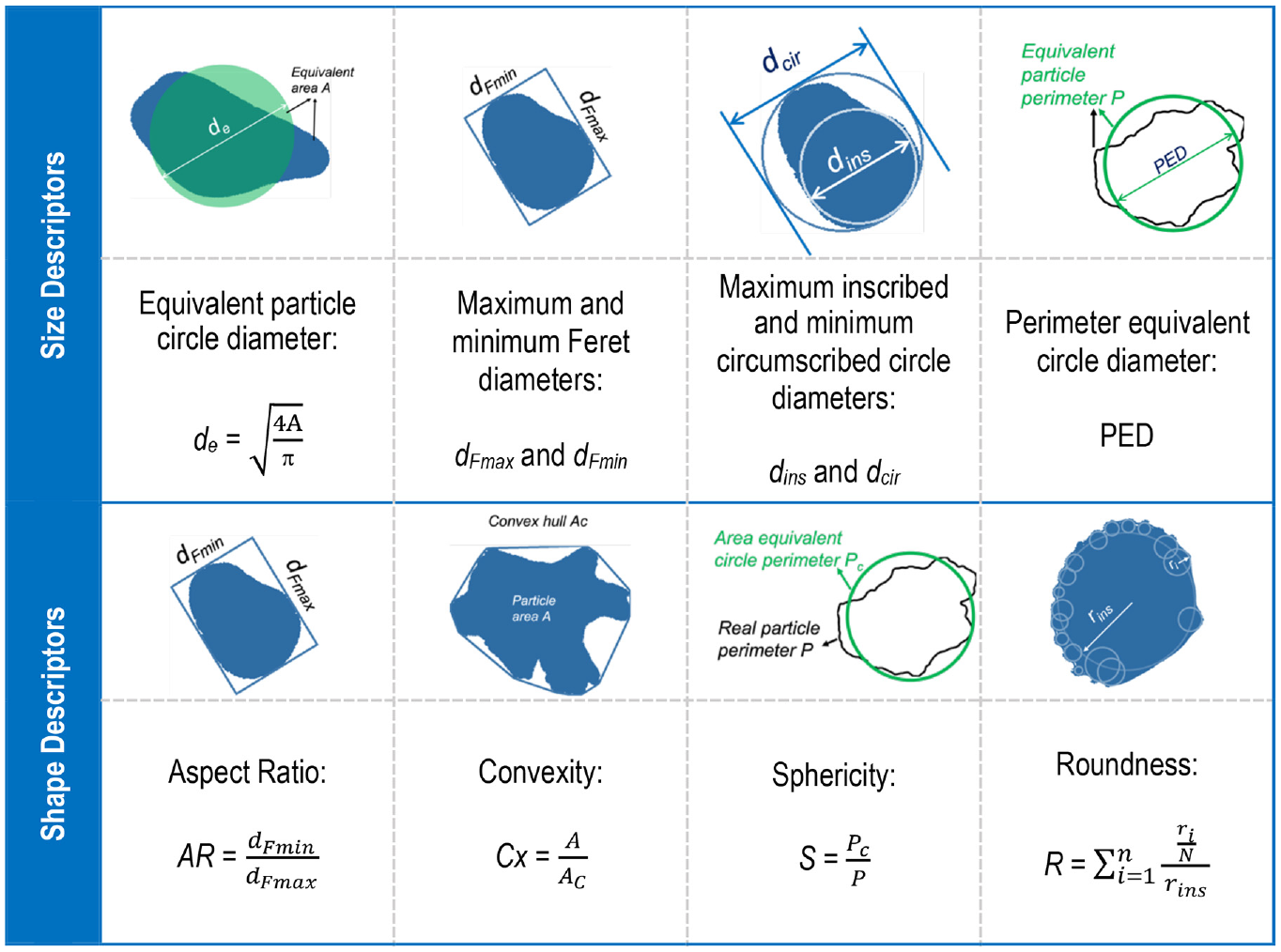
Particle size and shape descriptors.

These four shape and six size parameters were selected because: 1) they were previously shown to be independent of each other, 2) they are sufficient for classification analysis using ML, and 3) prior work has demonstrated that the highest classification accuracy was achieved when all 10 parameters were employed in the ML models ( 14 ).

Sands to Be Classified

Twenty sand specimens were utilized for analysis in this study. These sands were selected to cover a diverse range of sizes and shapes, effectively representing the intricate nature of sands encountered in classification scenarios. Details of the EQPC and Feret sizes, and shape descriptors, are available in Table 1. The information in Table 1 was acquired by the authors using DIA apparatus. These materials can be categorized as shown in Table 1.

Table 1.

Statistics of Shape and Size Descriptors Employed

Label	Metric	AR	Cx	S	R	d_e (µm)	D_Fmax (µm)	D_Fmin (µm)
Browse #1	Mean	0.62	0.87	0.62	0.65	476	673	414
Browse #1	SD	0.13	0.07	0.17	0.17	179	319	160
Cape Cod	Mean	0.72	0.95	0.83	0.65	575	712	508
Cape Cod	SD	0.12	0.03	0.06	0.10	242	294	218
Fiji pink	Mean	0.65	0.93	0.80	0.61	652	875	550
Fiji pink	SD	0.15	0.05	0.08	0.13	222	317	204
FRF	Mean	0.73	0.95	0.85	0.73	300	368	268
FRF	SD	0.10	0.02	0.05	0.09	66	86	61
Hawaii	Mean	0.70	0.92	0.76	0.41	1,459	1,865	1,306
Hawaii	SD	0.12	0.03	0.06	0.17	833	1,067	767
LBI, NJ	Mean	0.74	0.96	0.86	0.74	402	486	357
LBI, NJ	SD	0.10	0.02	0.05	0.09	103	133	94
Ledge Point	Mean	0.67	0.86	0.67	0.65	273	377	234
Ledge Point	SD	0.12	0.07	0.13	0.14	75	121	68
Ottawa #12-20	Mean	0.70	0.96	0.73	0.79	1,173	1,365	1,061
Ottawa #12-20	SD	0.10	0.02	0.12	0.10	217	280	201
Ottawa #20-30	Mean	0.79	0.96	0.78	0.79	824	952	745
Ottawa #20-30	SD	0.09	0.02	0.09	0.09	63	92	75
Ottawa #35-50	Mean	0.75	0.95	0.78	0.76	515	618	454
Ottawa #35-50	SD	0.10	0.03	0.10	0.08	101	137	93
Ottawa #40-70	Mean	0.74	0.94	0.77	0.77	355	429	315
Ottawa #40-70	SD	0.10	0.03	0.10	0.09	109	132	99
Ottawa #50-80	Mean	0.74	0.93	0.77	0.77	277	336	246
Ottawa #50-80	SD	0.10	0.04	0.10	0.09	64	80	59
Ottawa #70-100	Mean	0.76	0.91	0.75	0.73	290	358	262
Ottawa #70-100	SD	0.10	0.05	0.10	0.11	28	42	33
Oolite	Mean	0.70	0.94	0.83	0.73	307	390	268
Oolite	SD	0.13	0.04	0.07	0.11	84	120	76
Peace River	Mean	0.70	0.96	0.50	0.71	2,230	2,786	1,942
Peace River	SD	0.08	0.02	0.11	0.12	346	503	348
Quartz #4	Mean	0.62	0.93	0.38	0.62	1,770	2,458	1,495
Quartz #4	SD	0.09	0.03	0.08	0.14	273	464	307
Quartz #3	Mean	0.69	0.89	0.43	0.61	1,031	1,430	862
Quartz #3	SD	0.10	0.05	0.09	0.15	223	340	223
Quartz #2	Mean	0.70	0.82	0.57	0.63	342	492	283
Quartz #2	SD	0.12	0.08	0.12	0.15	93	148	87
Quartz #1	Mean	0.65	0.86	0.71	0.65	309	419	261
Quartz #1	SD	0.14	0.08	0.12	0.12	58	94	61
Vieques	Mean	0.67	0.95	0.83	0.59	585	756	498
Vieques	SD	0.13	0.02	0.05	0.11	202	278	180

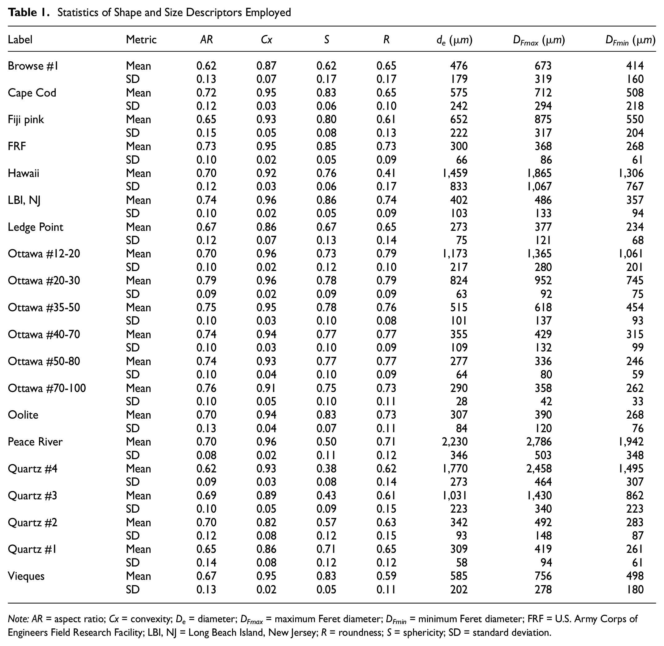
Note: AR = aspect ratio; Cx = convexity; D_e = diameter; D_Fmax = maximum Feret diameter; D_Fmin = minimum Feret diameter; FRF = U.S. Army Corps of Engineers Field Research Facility; LBI, NJ = Long Beach Island, New Jersey; R = roundness; S = sphericity; SD = standard deviation.

Machine-Sorted Sands

The following machine-sorted sediments were purchased from a materials supplier (Figure 3). All machine-sorted sands are poorly graded.

Ottawa #12-20, #20-30, #35-50, #40-70, #50-80 and #70-100 constitute naturally occurring siliceous sands that are mechanically sorted. Despite sharing uniformly rounded particle shapes, these sands are distinguished mainly by their sizes, as denoted by their passing and retaining sieves. Their respective median diameters D₅₀ were 1,276, 832, 565, 477, 317, and 295 µm, respectively.

Quartz #4, #3, #2, and #1 are sands made by mechanically crushing quartzite rock, each possessing a corresponding D₅₀ value of 1,861, 1,172, 411 and 317 µm, respectively. These sands exhibit an angular shape as a consequence of the crushing process.

Figure 3.

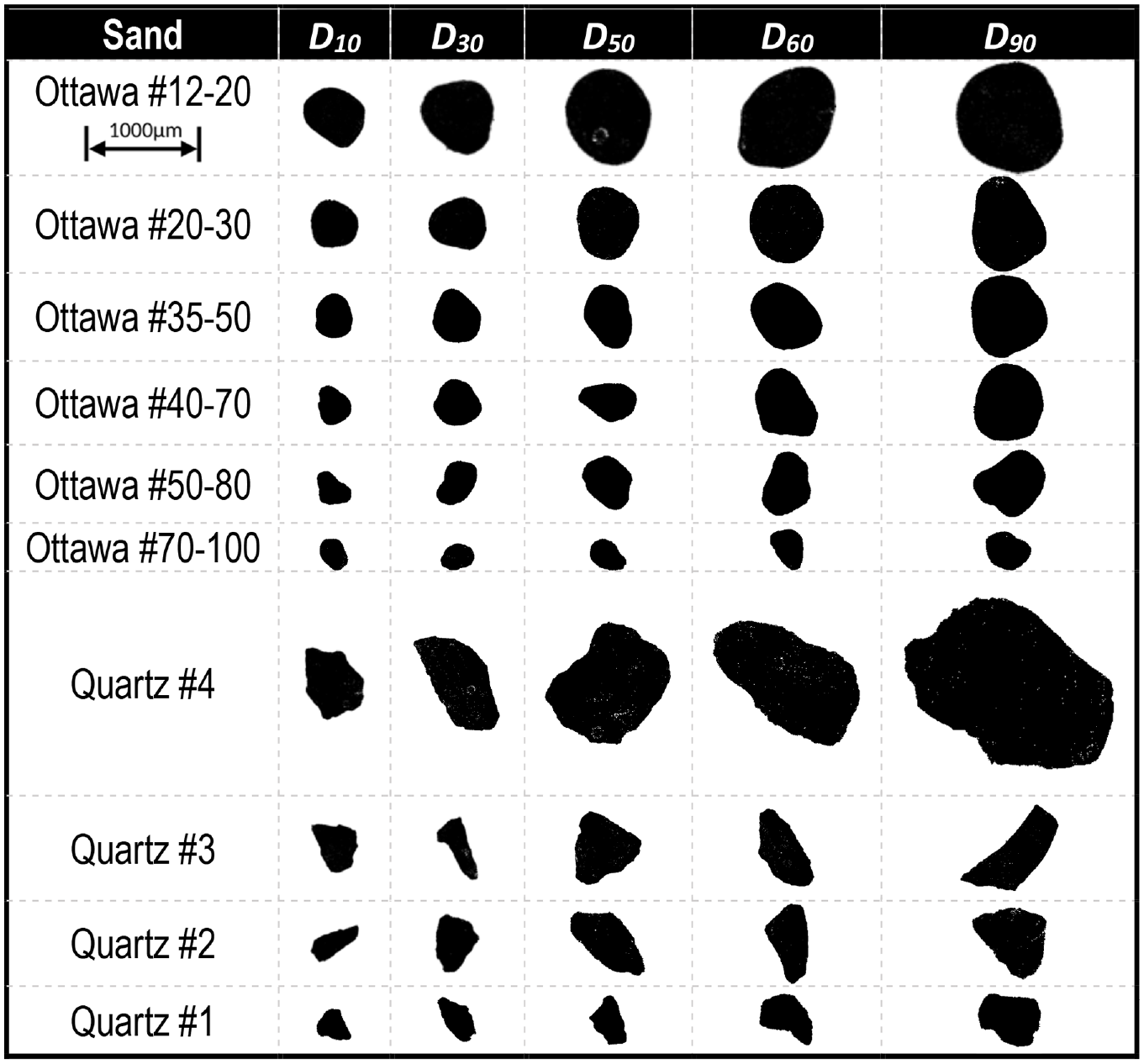
Dynamic image analysis images of 10 machine-sorted sands employed in this study.

Natural Sediments

Natural sand sediments were collected by the authors in an ad hoc process from a variety of beaches, suppliers, and research test sites (Figure 4).

Peace River sand is a feldspathic sediment found in nature which also serves as a decorative sand for aquariums. The supplier claims it originates from a river in Florida. This type of sand is composed of a blend of sub-angular and sub-rounded particles, with a D₅₀ measurement of 2,374 µm.

FRF is a sediment sourced from the U.S. Army Corps of Engineers Field Research Facility in Duck, North Carolina. It has a D₅₀ of 340 µm.

Vieques sand is utilized for research on sediment transport and erosion. It originates from Vieques Island in Puerto Rico. It has a D₅₀ of 821 µm.

LBI, NJ was collected from Ship Bottom beach on Long Beach Island in New Jersey. It has a D₅₀ of 2374 µm.

Oolite, Fiji pink, and Hawaii are naturally sorted calcareous sands, primarily intended for decorative use in aquariums. Each of these sands is rich in live bacteria and has distinct surface characteristics that enhance their extensive surface area, facilitating bacterial growth. The supplier specifies that Oolite originates from the Bahamas and is white in color, Fiji pink is a soft pink sand from an undisclosed location, and Hawaii is sourced from a live Hawaiian reef, featuring black sand. The three sands have D₅₀ measurements of 375 µm, 865 µm, and 2701 µm, respectively.

Cape Cod sand was obtained from a Woods Hole Oceanographic Institute research site 2.5 km southwest of Provincetown harbor. The sand originates from a sandbar that enjoys considerable protection from the open ocean and experiences limited exposure to Cape Cod Bay. This siliceous material has a relatively uniform composition, and a D₅₀ of 818 µm.

Browse #1 and Ledge Point represent intricate calcareous sediments sourced from Western Australia ( 16 ). These sands consist of shell fragments, imparting an irregular shape and the potential for intra-particle voids ( 17 ). While Browse #1 sand originates from a hemipelagic environment in deep water with low energy, Ledge Point sand is a coastal bioclastic sand originating from a high-energy shallow water environment. The materials have D₅₀ measurements of 689 µm and 316 µm, respectively.

Figure 4.

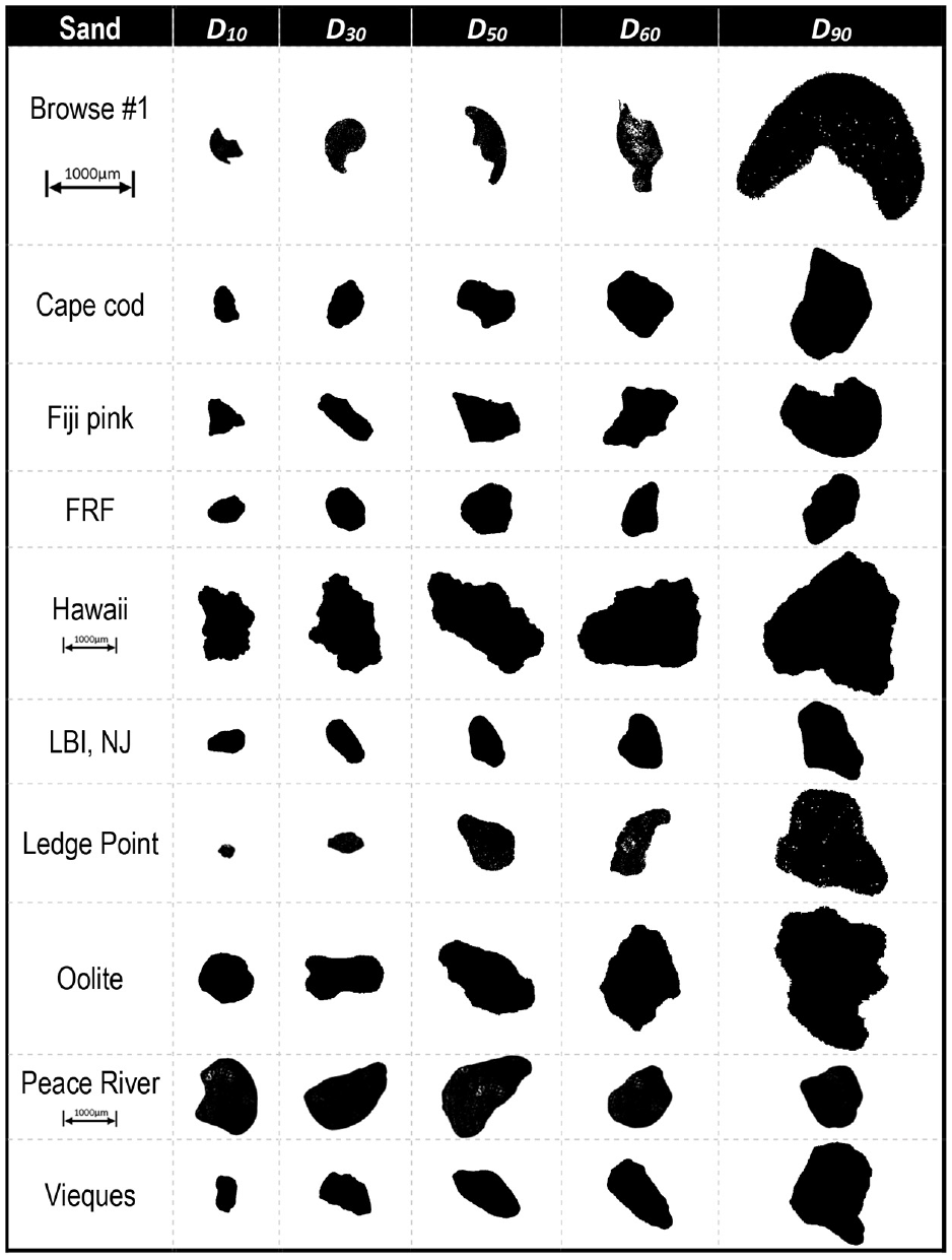
Dynamic image analysis images of 10 natural sands employed in this study.

Statistical Analysis of Dataset

A total of 2,000 particle images were captured by DIA for each type of sand, which resulted in a dataset consisting of 40,000 binary images. A QICPIC (Sympatec, Clausthal-Zellerfeld, Germany) equipped with an M7 camera lens was employed for capturing binary images with a resolution of 4 µm/px. Therefore, sand particles smaller than 200 µm were excluded from consideration since their image resolution was less than 50 pixels wide, which is not sufficient for meaningful analysis.

Representative DIA particle images of the 20 sands are shown in Figures 3 and 4. The cumulative particle size distributions of the 20 tested sands were computed from the EQPC diameter, illustrated in Figure 5. The distributions were represented using volume percentage for each sand. Volume distributions are believed to represent mass distributions obtained from sieve analysis as long as the material possesses a uniform specific gravity throughout the specimen.

Figure 5.

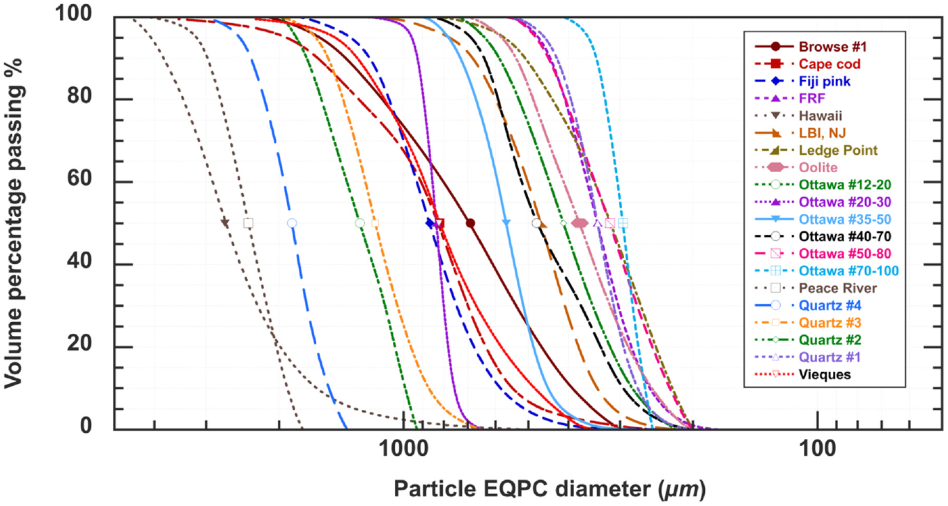
Particle size distribution of 20 classified sands.

All 20 sands are poorly graded, but they each possess a distinct size distribution. With the exceptions of Hawaii and Peace River sands, having D₅₀ values of 2,375 µm and 2,701 µm, respectively, the chosen sands possess median particle sizes with D₅₀ ranging from 316 µm to 1,861 µm. These sizes are categorized as fine-to-medium sands, while Hawaii and Peace River stand as the only coarse sands. Despite variations in particle size among the sands, identifying each sand solely by size would be challenging because of overlapping sizes across the various sands.

The statistical values of six typical size and four shape descriptors are presented in Table 1 for the 20 sands. All values are calculated using the size and shape descriptors obtained from DIA. A wide variety of shapes can be identified using the employed shape descriptors. The employed shape descriptors allow for the identification of a diverse array of particle shapes. The distribution of S and R values spans from 0.3 to 0.8, while AR values tend to fall within the range of 0.62 to 0.79. Notably, Cx displays the smallest standard deviation, with values consistently exceeding 0.82. These Cx values imply the absence of concave features on all sand surfaces, whereas AR values indicate that particles maintain a moderate level of elongation. Nevertheless, subtle distinctions also emerge among particles of similar sand types but varying sizes. For instance, in the case of Ottawa sands, #20-30 exhibits larger shape values compared with #40-70, despite both sands being classified as rounded according to the Krumbein-Sloss chart method ( 4 ). Similarly, calcareous sediments such as Oolite, Fiji pink, Hawaii, Browse #1, and Ledge Point display irregular particle shapes because of significant concavities and convexities on their surfaces. However, the angularity varies across these sands. In summary, it can be concluded that visually classifying the 20 examined natural sands poses a considerable challenge when relying on subjective visual observations, owing to their overlapping shape and size descriptors.

Machine Learning (ML) Classifiers

Several ML models were explored for classification of sands based on their sizes and shapes. All ML analyses were implemented using readily available packages in Python^®, as identified later. The following is a brief description of the ML models adopted in this work. More detailed description of these models is readily available in other papers ( 18 – 20 ). The classification task involves assigning one of 20 labels to each particle of sand, the labels being sand type (Table 1, Figures 3 and 4).

K-Nearest Neighbors (KNN)

K-nearest neighbor (KNN) classification algorithms make predictions about the class of a data point using a majority voting principle ( 21 ). Initially, the model is trained through by splitting the data into training and test sets. Next, the Euclidean distance is computed between the examined data points and the training dataset. In this process, K denotes the quantity of neighboring training points to incorporate into the classification process. The geometric distance dimensions are determined by the number of features present (with dimensions ranging from 4 to 60 in various analyses, encompassing up to six size and four shape attributes). The method presumes that instances within a dataset will generally exist in proximity to other instances that have similar properties. If the instances are tagged with a classification label, then the value of the label of an unclassified instance can be predicted based on the labels of its nearest neighbors. The distances from diverse shape and size parameters to the corresponding values in the particle being classified are thus utilized to classify individual particles. Consequently, the highest combined kernel densities were used for classification. The number of neighboring training points to be included in classification was taken in this study as K = 20, where 20 is the number of data points (i.e., particles) used for computing the nearest neighbor.

Support Vector Machines (SVM)

Support vector machines (SVM) have found extensive use in geotechnical applications for both classification and regression tasks, such as recognizing mineral grains automatically and predicting the axial load capacity of piles ( 22 – 24 ). The core principle behind SVM for classifying different entities involves identifying a hyperplane within the feature space. This hyperplane effectively separates distinct classes from one another. A crucial aspect is that the hyperplane should maximize its distance from the support vectors, which can represent diverse shape and size attributes, for instance. SVM classifiers face limitations when directly applied to classify multiple types of sands within a dataset. The approach involved classifying each individual type of sand against all other sands present. Consequently, this resulted in the creation of 190 binary sand classification models ( $C_{20}^{2}$ ), with each model categorizing the sand into one of two possibilities. To determine the final classification for a given sand type, a consensus was reached by considering the outcomes of all 190 models. For this study, an SVM employing a Gaussian kernel was chosen as the classification method.

Decision Tree

Decision tree is widely used in ML to produce a treelike model of decisions ( 25 ). It creates a tree-like model where each internal node represents a test or condition on an attribute, and each leaf node represents a class label (in classification). The tree structure is designed to help make decisions based on input features and learn patterns from the training data. In this study, shape and size features are employed as decision nodes. To identify the most favorable splits, a cost function is utilized. For instance, when a decision tree commences its splitting process, it evaluates each feature in the training data. The prediction for a specific group is derived by calculating the mean of the responses from the training data inputs within that group. A Gini score was employed to decide the efficacy of a split ( 26 ). Gini score calculates the probability that a feature is misclassified. The model computes the discrepancy between the Gini score before a split and the average Gini score after the dataset split, based on the given attribute values. A good split thus reduces the Gini score. Decision trees are interpretable, easy to visualize, and capable of capturing complex relationships in data. However, they are prone to overfitting, especially if they grow deep and complex trees. To mitigate this, techniques such as pruning (removing unnecessary branches) and using ensemble methods such as random forests are often employed.

Random Forest

Random forest is an ensemble learning technique that leverages the strengths of multiple decision trees to achieve improved predictive performance and generalization ( 27 ). It is particularly effective in handling complex datasets with high dimensionality and noise ( 28 ). The algorithm’s fundamental idea is to create a “forest” of decision trees, each trained on a different subset of the data and employing a subset of the available features. While growing each individual tree, the algorithm only considers a random subset of features for each node split. This feature selection randomness further contributes to the diversity of the trees. Once all the trees are trained, they collectively make predictions for new data points. For classification tasks, each tree “votes” for a class, and the class with the most votes becomes the final prediction. This method is widely used in various ML classifiers and can provide robust and accurate predictions.

Neural Networks (NNs)

NNs also known as Artificial Neural Network (ANN) are a classifier of ML model inspired by the structure and functioning of the human brain ( 29 ). They are designed to recognize patterns and relationships in data, making them particularly powerful for tasks such as image and speech recognition, natural language processing, and more. NNs consist of interconnected layers of nodes, also known as neurons, that process and transform input data to produce desired outputs. The basic building blocks of an NN are neurons. Neurons receive inputs, perform computations, and produce outputs. Neurons are organized into three types of layer. NNs have achieved state-of-the-art results in various fields but require substantial amounts of data and computation power for training. Advances in hardware and artificial intelligence techniques have enabled the development of more complex and efficient NN architectures, contributing to the rapid progress of deep learning research ( 30 , 31 ).

Ensemble Voting

Ensemble voting is a technique that involves combining distinct ML classifiers, each with its own unique concept, and leveraging a majority vote strategy to predict class labels. Ensemble voting is particularly useful when individual models perform well on different subsets of data or when they excel in different aspects of the task. It is a way to harness the power of diversity and collaboration to achieve better overall results. In majority voting, the anticipated class label for a specific sample corresponds to the class label that represents the most frequently occurring (mode) prediction across the individual classifiers. In this study, the five individual classifiers SVM, KNN, random forest, decision tree, and ANN were employed as an ensemble.

Results and Discussion

Five individual ML classifiers and the ensemble voting methods were employed for sand classification. In this study, 20 sands dataset with 40,000 ( $2, 000 \times 20$ ) particles in equal proportion were analyzed. The performance of the trained models, as well as the training and testing time, were compared in Table 2. All analyses were achieved using Python scripts developed by the authors with the aid of the Scikit Learn (SL) ML package, according to the methodology presented by Pedregosa et al. ( 32 ).

Table 2.

Test Accuracy and Efficacy of Different Machine Learning Models

Dataset	Total training time	Testing time	Test accuracy (%)
Dataset	Total training time	Testing time	Individual	Voting
Neural network
Size	13.7 s	0.006 s	46.1	85
Shape	15.7 s	0.009 s	28.9	75
Size and shape	14.8 s	0.006 s	48.8	90
Support vector machine
Size	13.3 s	2.922 s	42.9	NA
Shape	18.8 s	3.317 s	24.8	NA
Size and shape	14.2 s	2.827 s	45.6	75
Decision tree
Size	2.9 s	0.003 s	34.8	NA
Shape	2.9 s	0.003 s	17.6	NA
Size and shape	3.2 s	0.003 s	36.8	90
Random forest
Size	8.6 s	0.101 s	41.7	NA
Shape	6.6 s	0.146 s	22.9	NA
Size and shape	11.2 s	0.104 s	45.1	90
K-nearest neighbors
Size	2.6 s	0.041 s	39.6	NA
Shape	2.6 s	0.035 s	21.2	NA
Size and shape	2.7 s	0.049 s	40.9	75
Ensemble voting
Size	53.3 s	3.17 s	43.6	NA
Shape	61.7 s	3.54 s	25.1	NA
Size and shape	62.9 s	3.06 s	46.4	85

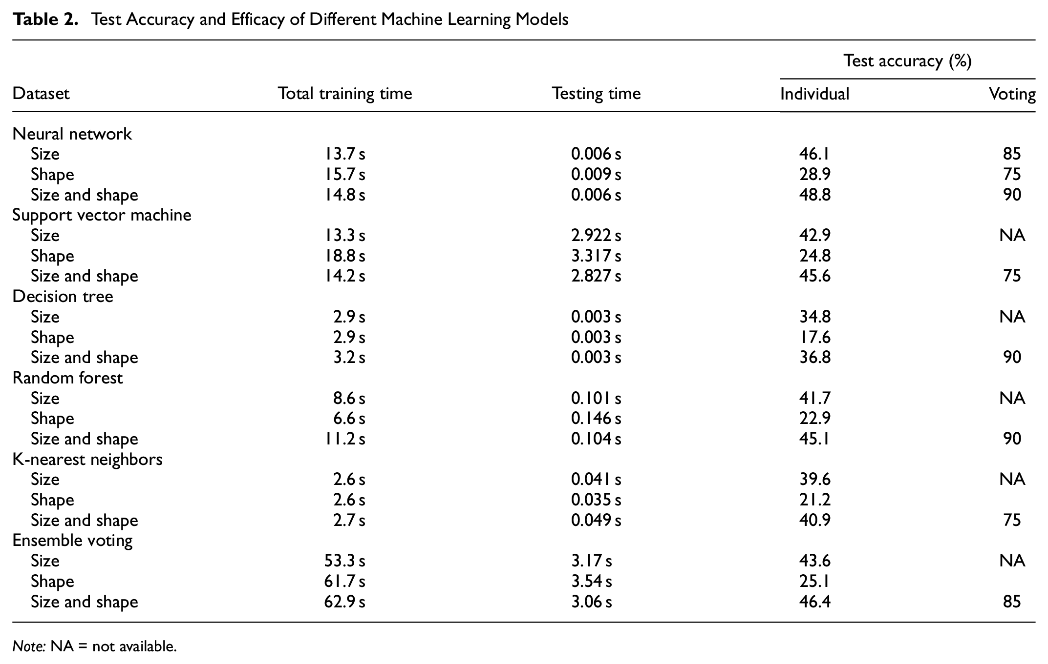
Note: NA = not available.

Feature scaling in ML is one of the fundamental techniques used for data pre-processing. It improves the performance and robustness of ML algorithms, such as KNN and SVM, by making uniform the Euclidean distance of size and shape features under consideration ( 33 ). Therefore, normalization and standardization were applied in the present study, as follows:

Normalization: the values of all size descriptors were normalized between 0 and 1. The smallest value of each size feature for all nine sands combined was assigned a value of zero, and the largest a value of 1. Values in between were linearly scaled.

Standardization (also known a Z-score) was implemented for both size and shape features by centering each data around the mean with a unit standard deviation, as $X^{'} = \frac{X - μ}{σ},$ where $μ$ and $σ$ are mean and standard deviation of feature values, respectively. The mean and standard deviation were computed for the entire specimen of 40,000 particles.

The performance of each classifier for sand particle classification was evaluated using mean accuracy, as shown in Table 2. Classification accuracy is defined as the ratio of the correctly predicted number of individual particles to the total number of sand particles. A 10-fold cross-validation was employed, by randomly splitting the dataset into 10 subsets, so that the test accuracy was performed using one subset ( $200 \times 20 sands = 4, 000$ data points) at each time and repeated 10 times. In each test the training dataset is $1, 800 \times 20 sands = 36, 000$ sand particles, which is 90% of the total dataset. This evaluation method ensures less overfitting and reduces the data points selection bias for fitting models ( 34 ).

In general, sand classification using size descriptors alone tends to yield better accuracy compared with using shape descriptors alone, across various ML classifiers. The average classification accuracy was 41.5% versus 23.4%. The reason is that the selected sands have a larger size variability compared with shape variability. The highest classification accuracy of 46.1% was achieved by employing an NN classifier using size-related features. On the other hand, when relying solely on shape features, the mean accuracy remains lower, falling within the range of 17.6% to 28.9%. When both size and shape features are combined in the ML models, the classification accuracy improves to 36.8%–48.8% using all classifiers. The greatest classification accuracy was observed using NNs with 48.8% of individual particles correctly classified. Engineering shape descriptors alone cannot differentiate the 20 examined sand particles well within the ML models. However, it is essential to combine size and shape descriptors together to reach the maximum accuracy. Finally, decision tree exhibited the lowest accuracy of 34.8%, 17.6%, and 36.8% using size, shape, combined size and shape together, respectively. Thus, the decision tree model is not suggested for solving individual sand classification problem.

Surprisingly, the application of ensemble methods did not significantly enhance classification accuracy compared with individual classifiers. For instance, the ensemble voting approach produced a slightly lower outcome than the individual NN classifier, yielding an overall accuracy of 43.6%, 25.1%, and 46.4% compared with 46.1%, 28.9%, and 48.8% using size, shape, size and shape together, respectively (Table 2).

Training time and testing time are also summarized in Table 2. All analyses were efficiently carried out on a personal MacBook Pro computer with an Apple M2 chip with 16 GB memory. The efficiency of the analyses can be attributed to the analyses employing numerical values representing shape and size features, rather than particle images. All algorithms were implemented using Python sklearn packages and were completed within a few seconds to 1 min. There is not a significant difference between using the number of features for classifying sands, but the ensemble voting method takes the longest computation time because of the necessity of iterating through each individual classifier. However, the maximum required time for training was 63 s.

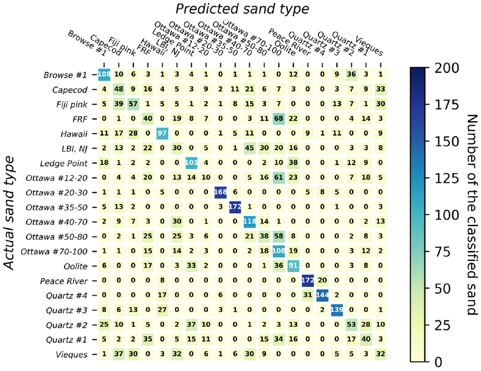
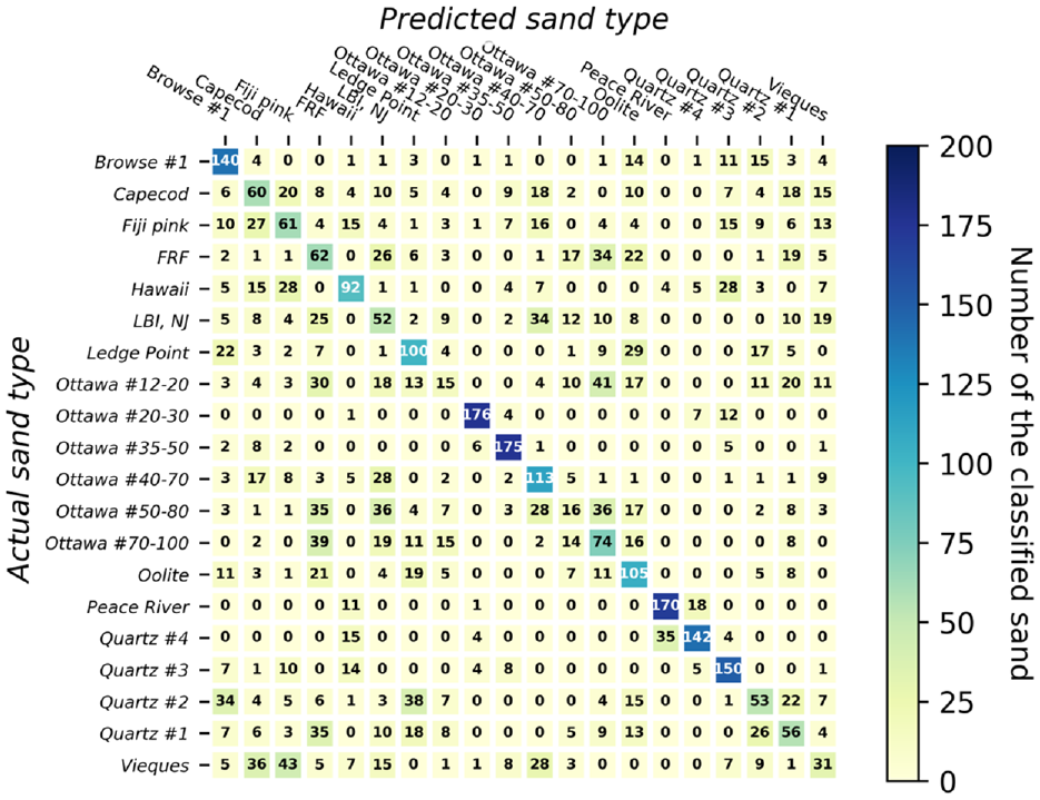
A confusion matrix, often referred to as an error map, serves as a visual representation that illustrates the performance of an ML algorithm. The matrix depicts the number of accurately classified particles corresponding to each specific type of sand within a dataset of 20 types of sand. Each row of the matrix corresponds to the actual sand type of instance, while each column corresponds to the predicted sand type. 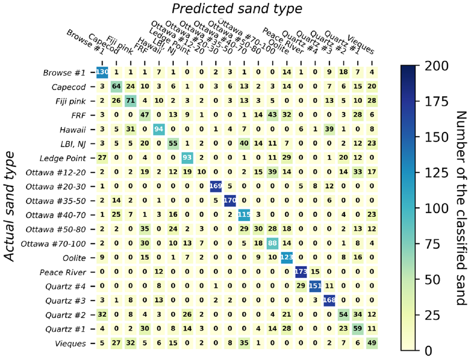In this study, the matrix comprises a grid with dimensions of $20 \times 20$ . Eight confusion matrices are presented in Figures 6 –13 corresponding to: 1) the test accuracy using each ML classifier with both size and shape features (Figures 6 –11), and 2) the test accuracy using NNs with size and shape features being the sole input (Figures 12 and 13).

Figure 6.

Predicted classification accuracy for 4,000 individual sand particles using neural networks employing size and shape descriptor data of each particle.

Figure 7.

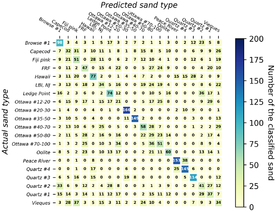
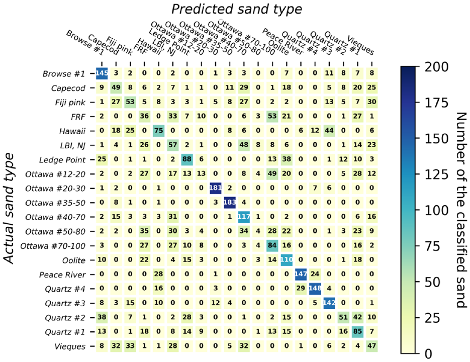
Predicted classification accuracy for 4,000 individual sand particles using support vector machine employing size and shape descriptor data of each particle.

Figure 8.

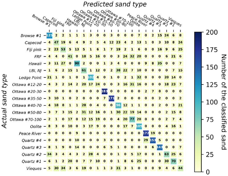
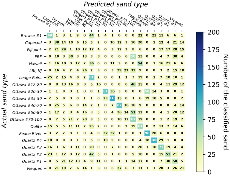
Predicted classification accuracy for 4,000 individual sand particles using decision tree algorithm employing size and shape descriptor data of each particle.

Figure 9.

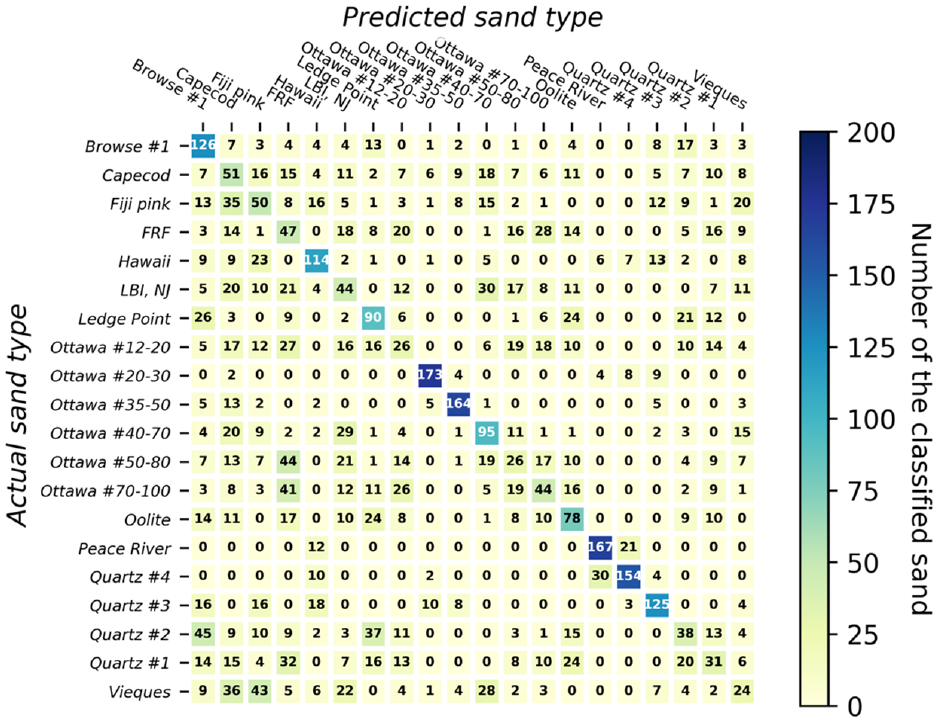
Predicted classification accuracy for 4,000 individual sand particles using the random forest algorithm employing size and shape descriptor data of each particle.

Figure 10.

Predicted classification accuracy for 4,000 individual sand particles using the K-nearest neighbor algorithm employing size and shape descriptor data of each particle.

Figure 11.

Predicted classification accuracy for 4,000 individual sand particles using the ensemble voting algorithm employing size and shape descriptor data of each particle.

Figure 12.

Predicted classification accuracy for 4,000 individual sand particles using neural networks employing size descriptor data of each particle only.

Figure 13.

Predicted classification accuracy for 4,000 individual sand particles using neural networks employing shape descriptor data of each particle only.

In Figures 6 –13, the numbers within each cell represent the number of classified particles falling into each respective category. The numbers on the diagonal of each matrix indicate the particles that were correctly identified for each sand type. Given that there were 200 particles of each sand type in the testing dataset, a perfect prediction would result in 200 particles along each diagonal. Values outside the diagonal indicate incorrectly classified sands, along with their corresponding misclassifications. For instance, the first row of the confusion matrix shown in Figure 6 indicates that, for Browse #1 sand, 130 (65%) out of 200 particles were correctly classified. However, 9%, 7%, 4.5%, 3.5%, and 2% were misclassified as Quartz #2, Oolite, Quartz #3, Quartz #1, and Vieques, respectively. Importantly, this does not imply a mixture of these sands within the specimen; it solely highlights the misidentification and the incorrect labels assigned.

An important observation is that, in nearly all cases, the majority of particles within each row can be accurately classified, as illustrated in Figures 6 –13 and Table 2. In particular, NN, decision tree, and random forest can classify 90% of 20 sand clusters using both size and shape. This performance is much better than classifying individual particles, as the accuracy rates for classifying individual particles were only 48.8%, 36.8%, and 45.1% for NN, decision tree, and random forest, respectively. On the other hand, as far as SVM, KNN, and ensemble voting are concerned, even though their accuracies are 75%, 75%, and 80%, respectively, their classification accuracy for sand clusters remains significantly better than classifying individual sands (which achieved accuracy of 45.6%, 40.9%, and 46.4%, respectively). Consequently, the probability of correctly classifying a sand cluster utilizing any of the six ML classifiers with both size and shape attributes is approximately 90%, according to the conducted tests.

When employing both size and shape features, NN demonstrated the highest classification accuracy compared with other classifiers. Additionally, utilizing a voting approach separately for size and shape features significantly improved the classification accuracy for individual sands (for size from 46.1% to 85%, and for shape from 28.9% to 75%). This demonstrates that ML has a remarkable ability to automatically classify sand clusters.

Some of the sands were identified with a very high accuracy by all models and some of them were not. For instance, Ottawa #20-30 and #35-50 and Peace River were consistently identified with the highest accuracies for all ML models, with an accuracy around 80%, while most of the natural soils and Ottawa #12-20 and Quartz #1 and #2 were not captured well. This is not related to the spread of the size and shape parameters. The relative standard deviation (standard deviation normalized by mean) of all parameters shown in Table 2 is presented in Table 3. The relative standard deviation of d_e and d_Fmax of the Vieques, for instance, is 35%–37%, while Peace River sand is around 16%–18% for the same parameters. One would expect the classification accuracy to improve with the decrease in the relative standard deviation, but that is not the case. A comparison between Vieques and Peace River (best- and worst-performing natural samples) suggests that the classification accuracy is not related to the relative standard deviation. Indeed, correlation between the relative standard deviation of the size or shape parameters with the best NN classifier suggests no correlation with R²<5% (not shown). Thus, ML algorithms are identifying relationships that are not evident through conventional statistical analyses.

Table 3.

Relative Standard Deviation (SD) of Shape and Size Descriptors Employed

Sand	Relative SD (%)							Average (%)			NN accuracy
	AR	Cx	S	R	d_e	d_Fmax	d_Fmin	Size and shape	Size	Shape	Individual	Cluster
Browse #1	21	8	27	26	38	47	39	29	41	24	65	True
Cape Cod	17	3	7	15	42	41	43	24	42	17	32	True
Fiji pink	23	5	10	21	34	36	37	24	36	19	36	True
FRF	14	2	6	12	22	23	23	15	23	11	24	True
Hawaii	17	3	8	41	57	57	59	35	58	25	47	True
LBI, NJ	14	2	6	12	26	27	26	16	26	12	28	True
Ledge Point	18	8	19	22	27	32	29	22	30	19	47	True
Ottawa #12-20	14	2	16	13	18	21	19	15	19	13	5	False
Ottawa #20-30	11	2	12	11	8	10	10	9	9	9	85	True
Ottawa #35-50	13	3	13	11	20	22	20	15	21	12	85	True
Ottawa #40-70	14	3	13	12	31	31	31	19	31	14	58	True
Ottawa #50-80	14	4	13	12	23	24	24	16	24	13	15	False
Ottawa #70-100	13	5	13	15	10	12	13	12	11	11	44	True
Oolite	19	4	8	15	27	31	28	19	29	15	62	True
Peace River	11	2	22	17	16	18	18	15	17	14	87	True
Quartz #4	15	3	21	23	15	19	21	17	18	15	76	True
Quartz #3	14	6	21	25	22	24	26	20	24	17	84	True
Quartz #2	17	10	21	24	27	30	31	23	29	20	27	True
Quartz #1	22	9	17	18	19	22	23	19	22	17	30	True
Vieques	19	2	6	19	35	37	36	22	36	16	25	True

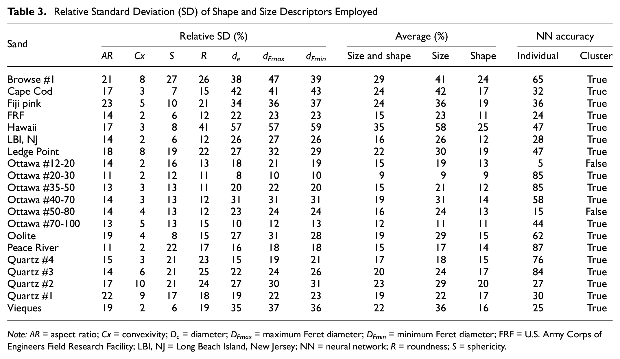
Note: AR = aspect ratio; Cx = convexivity; D_e = diameter; D_Fmax = maximum Feret diameter; D_Fmin = minimum Feret diameter; FRF = U.S. Army Corps of Engineers Field Research Facility; LBI, NJ = Long Beach Island, New Jersey; NN = neural network; R = roundness; S = sphericity.

It is possible to employ a voting algorithm where, when presented with a cluster of sand particles and their individual classifications, the predominant class within the cluster can be confidently identified as the sand type for that particular cluster. By comparing the highest count of sand particles classified within each row to the count of particles classified along the diagonal of the same row, comparing the greatest number of sand particles classified in each row with the number of particles classified along the diagonal of the same row is a metric for correct classification of a group of particles.

The problem at hand is an image classification problem which lends itself to analysis using convolution neural networks (CNN) ( 30 ). However, CNN is relatively time-consuming, and the proposed ML approach is much faster, from a numerical standpoint. The proposed ML models rely on engineering size and shape descriptors provided directly by the DIA software, eliminating the need for original images that CNNs requires. CNNs often demand extensive computational resources, taking approximately 2 h for training 50 epochs on a high-performance computing cluster. In contrast, our proposed ML models proved highly efficient as far as training time is concerned, requiring only a few minutes on a personal computer. Finally, our past research suggests that the classification accuracy of the majority of sand particles achieved with ML models is only slightly lower (10% lower) than CNN, demonstrating the effectiveness of ML for scaling up the work.

Conclusions

The feasibility of employing sand particle size and shape descriptors along with ML algorithms for sand classification has been demonstrated. Engineering size and shape descriptors were employed as features for sand particle classification using individual and ensemble ML models. The classification results show that the size and shape features are efficient and robust to identify up to 49% of individual sand particles, using parameters batch extracted from binary images. However, classification accuracy improved to 90% when clusters of particles were employed along with a voting algorithm. The next section provides a concise overview of the specific findings.

Among the ML models explored, NN provided the best performance for classifying 46.1%, 28.9%, and 48.8% of sand particles using size, shape, and size and shape descriptors, respectively.

For all the classifiers considered, size outperformed shape as a parameter for classification. However, use of combined size and shape parameters produced superior results for all sands and all classifiers.

Decision tree was the least accurate ML classifier and its use for soil classification is not warranted at this time.

A voting algorithm yielded a classification accuracy of 75%–90% for the 20 sands considered. It is noteworthy that engineering geologists commonly employ sand clusters in classification practice, and it is indeed unlikely that anyone would classify a particle of sand visually using a single particle. Thus, the performance of the voting regime is consistent with the accuracy attained by manual classification.

This work provides a basic and necessary step toward automatic machine classification of soils. In the future, the training dataset can be expanded from 20 to potentially hundreds of types of sand and enable quick soil classification on-site, during site investigation activities, using a smartphone equipped with a high-resolution camera. Indeed, reliable and speedy methods for segmentation of particles from images are also required, but research on these methods is ongoing (12).

These results suggest that ML promises to become commonly employed for classification of sand from ordinary images. Once appropriate segmentation algorithms are developed, and large libraries of sand particles are assembled, individual particles can be classified with approximately 40%–50% accuracy, and a voting algorithm can be used to classify the material based on the classification of the majority of individual particles. This method allows for automatic sand/particle classification which may eventually assist engineers on-site to quickly determine geotechnical properties of soil formations that would presently be analyzed in laboratories.

Footnotes

Author Contributions

The authors confirm contribution to the paper as follows: study conception and design: M. Iskander, L. Li; data collection: L. Li; analysis and interpretation of results: L. Li, M. Iskander; draft manuscript preparation: L. Li. All authors reviewed the results and approved the final version of the manuscript.

Declaration of Conflicting Interests

The author(s) declared no potential conflicts of interest with respect to the research, authorship, and/or publication of this article.

Funding

The author(s) received no financial support for the research, authorship, and/or publication of this article.

ORCID iDs

Linzhu Li

Magued Iskander

References

Cracknell

M. J.

Reading

A. M.

Geological Mapping Using Remote Sensing Data: A Comparison of Five Machine Learning Algorithms, Their Response to Variations in the Spatial Distribution of Training Data and the Use of Explicit Spatial Information. Computers & Geosciences, Vol. 63, 2014, pp. 22–33.

Sudarsan

Adamchuk

Biswas

Characterizing Soil Particle Sizes Using Wavelet Analysis of Microscope Images. Computers and Electronics in Agriculture, Vol. 148, 2018, pp. 217–225.

Iskander

Evaluation of Dynamic Image Analysis for Characterizing Granular Soils. Geotechnical Testing Journal, Vol. 43, No. 5, 2020, pp. 1149–1173.

Krumbein

W. C.

Sloss

L. L.

Stratigraphy and Sedimentation. Soil Science, Vol. 71, No. 5, 1951, p. 401.

Kim

Suh

H. S.

Yun

T. S.

Reliability and Applicability of the Krumbein-Sloss Chart for Estimating Geomechanical Properties in Sands. Engineering Geology, Vol. 248, 2019, pp. 117–123.

Liu

Gilbert

Cepeda

J. M.

Lysdahl

A. O. K.

Piciullo

Hefre

Lacasse

Modelling of Shallow Landslides with Machine Learning Algorithms. Geoscience Frontier, Vol. 12, No. 1, 2021, pp. 385–393.

McCoy

J. T.

Auret

Machine Learning Applications in Minerals Processing: A Review. Minerals Engineering, Vol. 132, 2019, pp. 95–109.

Shoji

Noguchi

Otsuki

Hino

Classification of Volcanic Ash Particles Using a Convolutional Neural Network and Probability. Scientific Reports, Vol. 8, No. 1, 2018, pp. 1–12.

Beucher

Rasmussen

C. B.

Moeslund

T. B.

Greve

M. H.

Interpretation of Convolutional Neural Networks for Acid Sulfate Soil Classification. Frontiers in Environmental Science, Vol. 9, 2022, p. 809995. https://doi.org/10.3389/fenvs.2021.809995.

10.

Kamilaris

Prenafeta-Boldú

F. X.

Deep Learning in Agriculture: A Survey. Computers and Electronics in Agriculture, Vol. 147, 2018, pp. 70–90. https://doi.org/10.1016/j.compag.2018.02.016.

11.

Azizi

Gilandeh

Y. A.

Mesri-Gundoshmian

Saleh-Bigdeli

A. A.

Moghaddam

H. A.

Classification of Soil Aggregates: A Novel Approach Based on Deep Learning. Soil and Tillage Research, Vol. 199, 2020, p. 104586. https://doi.org/10.1016/j.still.2020.104586.

12.

Hryciew

R. D.

Ghalib

A. M.

Raschke

S. A.

In-Situ Soil Characterization Using Vision Cone Penetrometer (VisCPT). In Geotechnical Site Characterization ( Robertson

P. K.

Mayne

P. W.

, eds.), Balkema, Rotterdam, The Netherlands, 1998, pp. 1081–1086.

13.

Iskander

Evaluation of Roundness Parameters in Use for Sand. Journal of Geotechnical and Geoenvironmental Engineering, Vol. 147, No. 9, 2021, p.04021081.

14.

Iskander

Use of Machine Learning for Classification of Sand Particles. Acta Geotechnica, Vol. 17, No. 10, 2022, pp. 1–21. https://doi.org/10.10071034/s11440-021-01443-y.

15.

Wadell

Sphericity and Roundness of Rock Particles. The Journal of Geology, Vol. 41, 1933, pp. 310–331.

16.

Beemer

R. D.

Bandini-Maeder

Shaw

Cassidy

M. J.

Volumetric Particle Size Distribution and Variable Granular Density Soils. Geotechnical Testing Journal, Vol. 43, No. 2, 2020, pp. 517–533.

17.

Beemer

R. D.

Iskander

Granulometry of Two Marine Calcareous Sands. Journal of Geotechnical and Geoenvironmental Engineering, Vol. 147, No. 3, 2021, p. 04020171.

18.

Mohri

Rostamizadeh

Talwalkar

Foundations of Machine Learning. MIT Press, Cambridge, 2018.

19.

Kodsy

Ozturk

Iskander

Forecasting of Pile Plugging Using Machine Learning. Acta Geotechnica, Vol. 18, 2023, pp. 3697–3714.

20.

Ozturk

Kodsy

Bazi

Iskander

M. G.

Efficacy of Several Design Methods for Predicting the Axial Compressive Capacity of Piles. Transportation Research Record: Journal of the Transportation Research Board, 2023. 2677: 1–17.

21.

Guo

Wang

Bell

Greer

KNN Model-Based Approach in Classification. In OTM Confederated International Conferences on the Move to Meaningful Internet Systems ( Meersman

Tari

Schmidt

D.C.

, eds.), Springer, Berlin, 2003, pp. 986–996.

22.

Carey

Boucher

Mahadevan

Bartholomew

Dyar

M. D.

Machine Learning Tools for Mineral Recognition and Classification from Raman Spectroscopy. Journal of Raman Spectroscopy, Vol. 46, No. 10, 2015, pp. 894–903.

23.

Machairas

N. P.

Iskander

M. G.

An Investigation of Pile Design Utilizing Advanced Data Analytics. Proc., IFCEE 2018, American Society of Civil Engineers, Reston, VA, 2018, pp. 132–141.

24.

Maitre

Bouchard

Be ÃÅdard

L. P.

Mineral Grains Recognition Using Computer Vision and Machine Learning. Computational Geosciences, Vol. 130, 2019, pp. 84–93.

25.

Friedl

M. A.

Brodley Decision

C. E.

Tree Classification of Land Cover from Remotely Sensed Data. Remote Sensing of Environment,Vol. 61, No. 3, 1997, pp. 399–409.

26.

Myles

A. J.

Feudale

R. N.

Liu

Woody

N. A.

Brown

S. D.

An Introduction to Decision Tree Modeling. Journal of Chemometrics: A Journal of the Chemometrics Society, Vol. 18, No. 6, 2004, pp. 275–285.

27.

Belgiu

Drăguţ

Random Forest in Remote Sensing: A Review of Applications and Future Directions. ISPRS Journal of Photogrammetry and Remote Sensing, Vol. 114, 2016, pp. 24–31.

28.

Rigatti

S. J.

Random Forest. Journal of Insurance Medicine, Vol. 47, No. 1, 2017, pp. 31–39.

29.

Shahin

M. A.

Jaksa

M. B.

Maier

H. R.

Artificial Neural Network Applications in Geotechnical Engineering. Australian Geomechanics, Vol. 36, No. 1, 2001, pp. 49–62.

30.

Iskander

Classification of Sands Using Deep Learning. Journal of Geotechnical and Geoenvironmental Engineering, Vol. 149, No. 11, 2023, p. 04023103.

31.

Machairas

Iskander

Application of Dynamic Image Analysis to Sand Particle Classification Using Deep Learning. Proc., Geo-Congress 2020: Modeling, Geomaterials, and Site Characterization, American Society of Civil Engineers, Reston, VA, 2020, pp. 612–621.

32.

Pedregosa

Varoquaux

Gramfort

Michel

Thirion

Grisel

Vanderplas

Scikit-Learn: Machine Learning in Python. Journal of Machine Learning Research, Vol. 12, 2011, pp. 2825–2830.

33.

Zheng

Casari

Feature Engineering for Machine Learning: Principles and Techniques for Data Scientists. O’Reilly Media, Inc., Newton, MA, 2018.

34.

Fushiki

Estimation of Prediction Error by Using K-Fold Cross-Validation. Statistics and Computing, Vol. 21, 2011, pp. 137–146.