Effects of Driver Gender,Driving Experience,and Visibility on Car-Following Behavior

Abstract

Weather visibility interference has a significant impact on driver car-following behavior. To investigate drivers’ car-following behavior and emergency avoidance behaviors under different visibility disturbances, scenarios are constructed under different foggy concentration environments based on driving simulation, and the drivers’ response behaviors are collected in the stable car-following state and emergency rear-end scenarios. Exploring the differential effects of gender and driving experience on driving behavior for fog concentrations based on multifactorial analysis of variance. A quantitative model of car-following risk is constructed based on factor analysis, and a linear mixed model is used to explore the comprehensive effects of fog concentration, speed, and the following distance at the braking time on drivers’ braking reaction time by fully considering the differences in individual behaviors. The results show that driving behavior is significantly affected by visual visibility, driver’s gender, and driving experience. With the decrease of visibility, following driving speed decreases, the following distance is shortened, the headway decreases, and the standard deviation of lane lateral offset distance increases. The rear-end collision risk of an experienced driver is higher than that of a novice driver, and the rear-end collision risk of the female is higher than that of male. The risk of collision is higher when traveling in light fog. In emergency rear-end collision scenarios, as visibility decreases, braking reaction time increases, and the risk of collision conflict increases at the moment of driver braking. The braking reaction time of the driver decreases with the increase of the speed and increases with the increase of the distance when the front vehicle is braking. The results of this study provide theoretical support and technical reference for effectively improving driving safety in a bad-visibility environment.

Keywords

pedestrians bicycles human factors human factors of vehicles driver behavior

In the traffic system composed of humans, vehicles, and road environment, environmental factors play a vital role in traffic safety. Compared with sunny weather, driving in bad weather conditions has an important impact on driving behavior, which increases the risk of crashes. This has been widely discussed ( 1 – 4 ).

The impact of bad weather conditions on different traffic environments varies ( 5 ). With the continuous development of the economy and the increasing number of automobiles, the car-following state is most frequently in the urban road environment. The operating status of the leading vehicle (LV) has a significant effect on the behavior of the rear driver ( 6 , 7 ). When the distance between the two vehicles is small, if the LV emergency brakes, the rear driver cannot take measures timely and effectively to avoid collision, easily causing rear-end crashes ( 8 ). Studies have shown that distracted driving, risky driving behaviors, and environmental visibility of the rear-end driver during the driving process all contribute to rear-end collisions, and are more likely to lead to multi-vehicle rear-end crashes ( 9 – 11 ). Therefore, it is necessary to explore the characteristics of car-following behavior to avoid rear-end collisions. At the same time, the study of car-following behavior can also provide an effective theoretical basis for vehicle forward collision avoidance, traffic simulation, capacity estimation, and the construction of intelligent transportation systems ( 12 ).

During vehicle driving, drivers obtain most of the information through visual perception ( 13 ). Foggy days—a kind of unfavorable weather that has a great negative impact on drivers’ visual perception—are the most dangerous for driving and most likely to cause drivers’ to panic ( 14 ). In addition to the impact of visual distraction, bad visual distance conditions are also one of the important causes of traffic accidents. In low-visibility foggy conditions, the drivers’ visual distance will be greatly reduced with the rise of fog concentrations ( 15 ). Further, when driving in foggy conditions, the drivers’ surrounding environment, traffic markings, and front vehicles are difficult to distinguish; at the same time, fog will scatter light and absorb light, resulting in reduced object brightness and more unfavorable observation, making it easy for drivers to make decision mistakes (16 –18). Driving in foggy conditions will also increase the psychological workload of drivers, resulting in abnormal driving behaviors, which may interfere with adjacent lanes, reduce road traffic capacity, and have a certain impact on the stability of the entire road traffic system ( 19 ).

When driving in a foggy environment, the driver’s attention is focused on the nearby area, resulting in a more concentrated visual search area ( 20 ). As driving time increases, drivers are prone to distraction, fatigue, and other adverse driving states. Studies have shown that the possibility of rear-end collision increases with the reduction of visibility ( 21 , 22 ). Crashes in low-visibility environments are more likely to lead to serious consequences than those occurring when visibility is good ( 23 , 24 ). Although foggy weather causes traffic to decrease, it causes an increase in the number of injury crashes ( 25 ). Therefore, it is necessary to pay attention to the safety of car-following behavior in a low-visibility environment ( 26 ).

Fog will have an important impact on drivers’ behavior. When visibility is lower than a certain threshold, drivers will significantly reduce their driving speed ( 27 , 28 ). However, because drivers tend to reduce the following distance, there is not enough distance to slow down, increasing the risk of rear-end collision ( 29 ). Based on cellular automata, Liu et al. established a microscopic model of car-following and lane-changing traffic flow under fog conditions and found that the speed fluctuated greatly in medium fog, the speed dispersion in dense fog was large, and the number of lane-changes decreased with the fog concentration increase ( 30 ). Based on simulated driving tests, Gao et al. found that the driver’s change of speed and distance difference in low visibility weather is different from that on sunny days ( 31 ). Kang et al. explored the effect of visibility on car-following behavior based on driving simulation tests and found that it is more difficult for the driver to respond to the change of LV speed than to the change of headway ( 32 ). Huang et al. found that the following distance increased with decreasing fog density and increasing speed limit, by designing a simulation test of the car-following behavior under different fog concentrations ( 33 ). Based on historical crash data, there is a correlation between low-visibility environments and vehicle crash rates ( 34 ).

Cognitive behavior theory suggests that human behavior is based on certain information generated through brain decision-making ( 35 ). In the driving process, because of the visibility decrease in foggy environments, the distance at which drivers can perceive danger is much shorter than in normal conditions ( 36 ). Driving in low visibility conditions is dangerous for drivers of all ability levels, but not all drivers are equally affected ( 37 ). Some drivers will reduce their speed in low-visibility conditions so that they can obtain a longer reaction time to react to the danger, while young and inexperienced drivers will choose to hardly reduce their speed ( 38 , 39 ). In addition, age differences will lead to different behaviors, and elderly drivers may face greater collision risk under high fog density and moderate speed ( 40 ). This is mainly because drivers’ behavior is influenced by their characteristics such as gender, age, and driving experience ( 41 ). In related research, driving simulation technology is widely used. It has the advantages of realistic effect, energy-saving, safety, and economy, and is not limited by time, climate, and site ( 42 ). In addition, many scholars have verified that this method has a high consistency with the results of real vehicle tests ( 43 ).

Although many studies have been conducted on the influence of foggy conditions on driving behavior and traffic safety, the inherent law of the relationship between urban road car-following behavior and visual characteristics needs to be further explored. The interaction effect of driving speed and visibility environment on car-following behavior has not been studied. To explore the effects of road visibility, driver characteristics, and driving speed on car-following behavior, this study of car-following behavior on urban roads under a foggy environment will construct virtual test scenarios from the perspective of driver visual cognition, with the idea that a foggy environment affects driver vision, and then influences driving behavior. Based on the scenario, the behavioral characteristics of drivers driving under different visibility interference are explored, providing theoretical support for the safe driving of drivers under foggy environments.

The rest of this paper is structured as follows. The next section describes the experimental design process of the driving simulator research. The results are analyzed and discussed in the section after that, and the final section provides concluding remarks and suggestions for future works.

Methodology

Apparatus

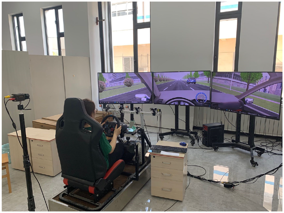
This study uses the driving simulator system as shown in Figure 1. The driving simulator system consists of hardware and software. The hardware of the driving simulator system includes: 1) a triple-screen display, consisting of three LED liquid crystal displays, which can be combined to provide a 135° driving field of view—each screen is 55 in., with a resolution of 1920 × 1080 and a 60 Hz refresh rate, and it is used to present a virtual driving scene; 2) the driving system, consisting of the driver’s seat, steering wheel, and pedals—used to simulate the actual driving environment, through which the system can realize the driver’s manipulation and control of the vehicle in the simulation scene; and 3) audio—embedded in the triple-screen display—used to play the ambient sound, vehicle engine sound, and so forth when driving the vehicle.

Figure 1.

Apparatus.

In this study, the virtual driving scenario was constructed using the UC-Win/Road 14.0 driving simulation system software. This is a three-dimensional traffic scene design software launched by the Japanese company FORUM8. The software can define and edit the road as necessary. Also, on the traffic network environment, road participants’ driving trajectory, and form of design definition, the software has a wealth of built-in vehicles, road facilities, and road participant models, available to the software user for the construction of the driving environment. The log plug-in of the software can record the coordinate position, driving direction, speed, acceleration, and lateral offset distance of the subject vehicle and its surrounding vehicles at a data collection frequency of 25 Hz, and save the output as a CSV-format file, which is convenient for data recording and post-processing analysis.

Procedure

Based on the UC-Win/Road driving simulation software, the concentration of fog was set to realize the simulated driving scenarios under different visibilities. During the experiment, the driver maneuvered the vehicle on a two-way six-lane urban road. The rear car and the front car are ordinary cars, and the visibility is set to three driving environments, as shown in Figure 2: light fog (visibility of 250 m), dense fog (visibility of 50 m), and sunny (no fog). The speed of the LV is set to 60 km/h, 40 km/h, and 20 km/h, and the road shape is set to straight and curved, which constitutes a total of six driving scenarios. The driving route is shown in Figure 3.

Figure 2.

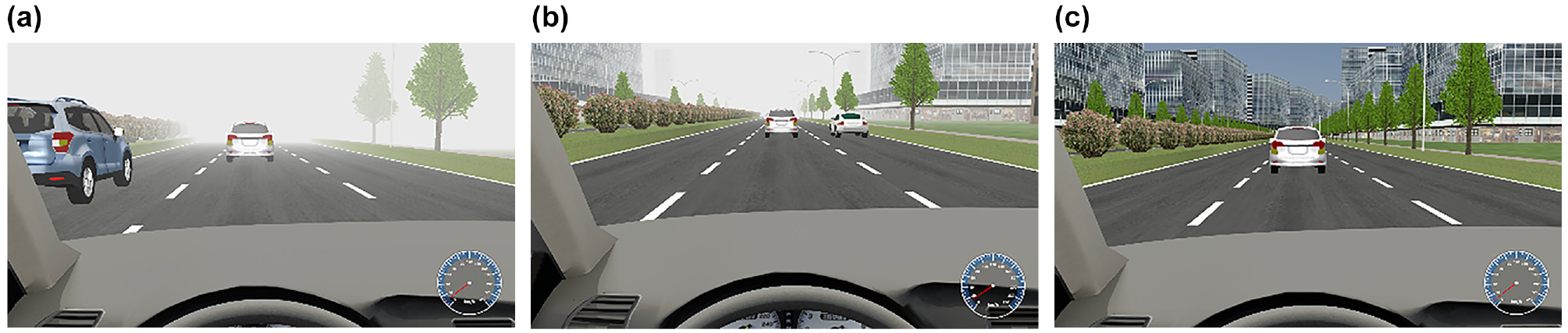
Foggy driving simulation scenarios: (a) Dense fog, (b) Light fog, and (c) No fog.

Figure 3.

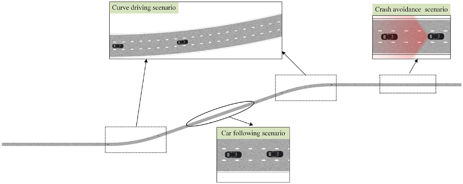
Schematic diagram of simulated driving routes.

The LV deceleration trigger point is set on the driving road, to trigger the braking and deceleration behavior of the LV. To approximate the actual traffic driving scenario, 500 passenger car units per hour (pcph) traffic flow was set up in the opposite lane of the experimental road, and 150 pcph traffic flow was set up in the adjacent lane in the same driving direction. The subjects were given practice through simulated driving to adapt to the driving environment and driving operation in foggy environments. During the experiment, the drivers were required to keep following the vehicle in the middle lane under the premise of obeying the traffic rules.

To calibrate the relationship between fog concentration and different visibilities in driving scenarios, the calibration process of 50 m visibility was taken as an example. Eight drivers with normal vision were selected, and a sedan was placed directly in front of them on the test road. The distance between the driver and the car is set to 50 m, and the fog concentration is set at a point where the driver can just see the outline of the front vehicle, and the fog concentration parameter value of this state is recorded. Finally, the average value of fog concentration parameters obtained by eight drivers was taken as the fog concentration value of 50 m visibility in the formal test process, and the visibility of other fog concentrations could be calibrated similarly.

Participants

Driver recruitment information was published through the website of Chang’an University, and test drivers who met certain conditions were recruited in Xi’an, China. All drivers were required to obtain a legal driver’s license, have a good mental state when participating in the experiment, have no physiological diseases, have normal vision or normal after correction, and have no drinking, drug-taking, staying up late, and other behaviors within 48 h before the experiment. The experimental settings and design were performed following relevant guidelines and regulations published by the Chinese Psychological Society (https://www.cpsbeijing.org/). This study involves the visual characteristics of drivers. Considering the influence of age on the visual characteristics of drivers, the age difference of the tested driver group should not be too large ( 44 ). A power analysis was performed for sample size estimation using G*Power 3.1. For repeated measures analysis of variance (ANOVA) (within factors) with four groups and three conditions, a required sample size of 33 was estimated, given the effect size of 0.3, an alpha of 0.05, and a power of 0.8. Considering the purpose, duration, and cost of the experiment, a total of 34 subjects were randomly recruited, including 23 males and 11 females, aged between 19 and 28 years old. Drivers with less than 3 years of driving experience are classified as novice drivers, and those with more than 3 years are classified as experienced drivers, so there are 17 novice drivers and 17 experienced drivers ( 45 – 47 ).

Design and Procedure

Before the start of the experiment, the researchers introduced the basic requirements of the experiment and the road scene to the subjects and told the drivers to drive according to their habits. During the experiment, the drivers should control the vehicle and keep following the LV. Under the premise of safety, the drivers were required to keep a relatively close following distance with the front car, as far as possible. The driver is not allowed to change lanes or overtake vehicles throughout the experiment. The experimental process is as follows:

1) Debugging the equipment of the driving simulation test platform before the experiment to ensure operation. The subjects were orally asked whether they satisfied the basic requirements of driving required by the experiment.

2) The subjects completed the statistical table of demographic factors, including name, gender, age, and driving experience. Then guide the subject to the driving simulator equipment, to adjust the seat to a comfortable position, explain the experimental precautions and equipment operation methods, guide the subject to carry out about 6 min of adaptive exercises in the practice scene, to master the steering wheel, pedal, and other vehicle control operation methods. Generally, experienced drivers take less time than novice drivers to become familiar with simulated driving operations.

3) After the subject is familiar with the driving operation, the experiment will be terminated if the driver is in discomfort. Ensure that the driver participating in the formal test is comfortable with the simulated driving environment.

4) After the end of the adaptive exercise, the driver takes a short rest to enter the formal test.

At the end of each scenario, the experimenter exported and saved the driving behavior data, and the subjects could choose whether they needed to take a break to prevent fatigue. The relevant instructions used for the subjects during the experiment were required to be consistent. There were three sub-experiments in the formal experiment, and the driving order of each scenario was randomly selected.

Results and Discussion

Based on different research purposes, there are differences in the criteria for determining the car-following state. Lochrane et al. used following time greater than 20 s and following distance less than 80 m as the criteria for determining car following ( 48 ). The criteria for Hammit’s selection were a following time of more than 20 s and a following distance of less than 60 m ( 49 ). Based on previous studies, combined with the actual situation of the experiment, the criterion for determining the car following in this study is that the driver’s stable following time is more than 20 s and the LV is maintained within the visible range.

To more comprehensively describe the driving behavior characteristics in car-following scenarios, based on the test data obtained from the experiments, the effects of different visibilities on the characteristics of drivers’ following behaviors were investigated from the indicators of speed, standard deviation (SD) of speed, following distance, headway, and the SD of the vehicle’s lateral offset distance.

By analyzing the correlation between the following distance and visibility, it was found that some drivers adopted positive strategies in foggy conditions to keep the front vehicle within sight, while some drivers adopted negative attitudes under the influence of fog and speed of the front vehicle, which caused the front vehicle to drive out of the vision field. Statistical analysis found that in the dense fog environment when the front vehicle is traveling at 60 km/h, 26.47% of the drivers adopt a following distance greater than the visibility of 50 m, that is, the front vehicle disappears from the driver’s field of vision. In the dense fog environment when the front vehicle is traveling at 40 km/h, 11.76% of the drivers adopt a following distance greater than the visibility of 50 m. When the front vehicle is traveling at 20 km/h, all the drivers adopt a following distance less than the visibility of 50 m. This shows that there are obvious differences in drivers’ behavior in low-visibility environments. However, overall, as visibility decreases, drivers tend to reduce the following distance to keep the front car in visual range as much as possible. Studies have shown that, if the front vehicle disappears from the rear driver’s view, it can easily create a sense of danger for the following driver ( 50 ). Since this study focuses on the status of the car following, only the leading vehicles that remained within the driver’s visibility were analyzed further.

Characteristics of Car-Following State

Following Distance

The following distance reflects the driver’s ability to control the distance, and their safety awareness. A three-way ANOVA was used to investigate the effects of driving experience, gender, and visibility on the following distance, and the interaction of the three factors and the interaction of the two factors of three had no significant effect on the following distance (all p > 0.05). However, the main effect of visibility was significant (F = 10.512, p < 0.01). With the visibility decrease, the following distance decreased significantly. The main effect of driving experience was also significant (F = 8.40, p = 0.004 < 0.01), with novice drivers having a significantly greater following distance than experienced drivers, with a mean difference of 11.248 m. However, the main effect of gender was not significant (F = 0.072, p = 0.789 > 0.05); female drivers had a greater following distance than males, with a mean difference of 1.04 m.

Headway

Headway can reflect the driver’s radical degree, but also directly reflects the driving habits ( 51 ). The distribution of headway in different foggy environments is shown in Figure 4. It can be seen that the effect of foggy concentration on headway is obvious, and drivers will choose a smaller headway when following a vehicle in lower visibility conditions. This is because fog reduces the visual stimulation of the surroundings, which leads to the driver’s misjudgment of the LV speed, and the tendency to reduce headway because of the expectation of keeping the front vehicle in the visible range. In a no-fog environment, as the speed of the front vehicle decreases, the driver tends to take a smaller headway. This is because the driver’s sense of crisis when following the vehicle decreases, so they take a smaller headway when the speed is lower. In a foggy environment, when the front vehicle speed is 40 km/h, the average value of the headway is less than the headway taken when the front vehicle speed is 20 km/h. Especially in a dense-fog environment, the driver takes a smaller headway to keep the visibility of the front vehicle, which is prone to cause a rear-end collision because of insufficient safety distance.

Figure 4.

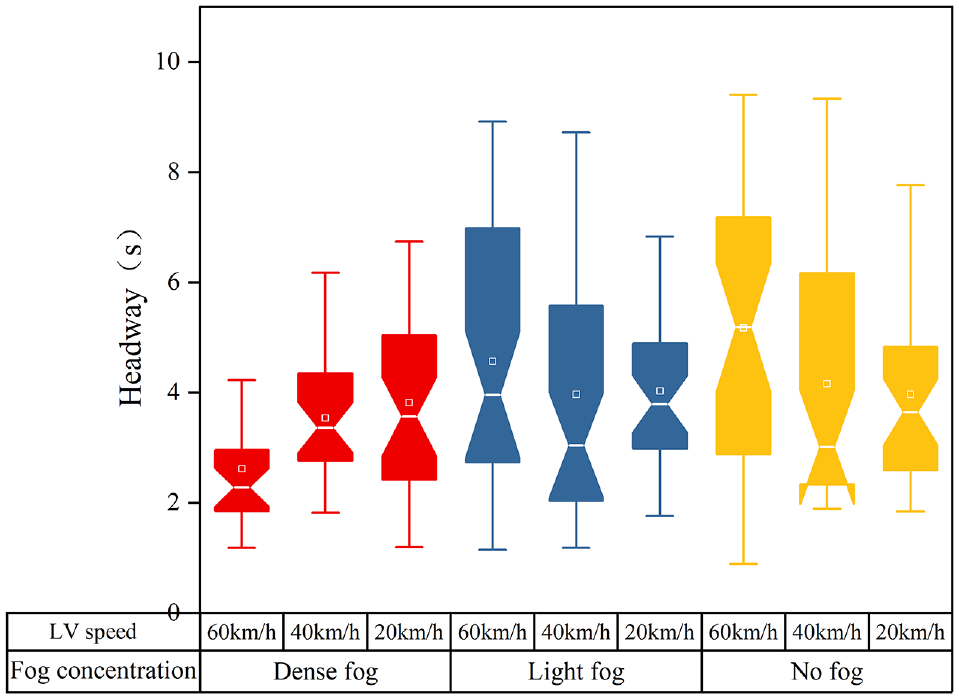
Headway under different fog conditions.

The three-way ANOVA results for visibility, gender, and driving experience showed a significant main effect of visibility (F = 5.752, p = 0.004 < 0.05) and, as the fog concentration increased, the driver’s visibility decreased, and the headway was significantly lower (M = 4.473 s for no fog, M = 4.115 s for light fog, M = 3.393 s for dense fog). The main effect of driving experience was also significant (F = 15.558, p < 0.01), with novice drivers having greater headway than experienced drivers, with a mean difference of 0.967 s.

Speed and Standard Deviation (SD) of Speed

Under the interaction of different fog concentrations and the front vehicle speed, the speed and the SD of the speed are shown in Figure 5. Comparative analysis reveals that speed is the highest when driving in a no-fog environment and, with the reduction of visibility, the driver tends to reduce speed; the SD of speed is the largest in the light-fog environment. A three-way ANOVA was used to investigate the effects of the three factors of driving experience, gender, and visibility on the SD of speed, and it was found that there was no significant effect of the three-factor interaction, the two-factor interaction, and the main effect of each factor on the SD of speed (all p > 0.05).

Figure 5.

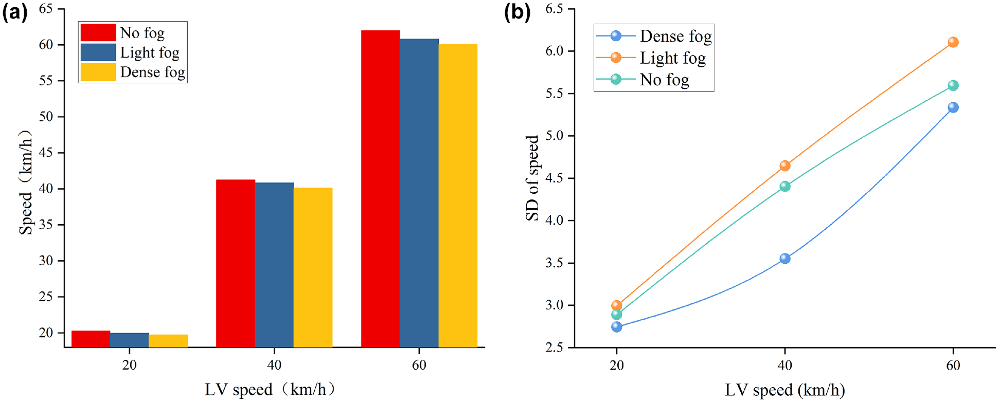
Characteristic analysis of (a) following speed and (b) SD of speed under different visibilities in foggy environment.

Standard Deviation (SD) of Following Distance

The SD of the following distance can reflect the fluctuation degree of the following distance in the driving process. As can be seen from Figure 6, under the condition of the same LV speed, the SD of the following distance decreases with the increase of the fog concentration, and the higher the following speed, the higher the SD of the following distance. Combined with the analysis of speed and the following distance, the analysis shows that the speed was high in the no-fog environment; the following distance and its SD were large. The speed was low when driving in a dense-fog environment; the following distance and its SD were small.

Figure 6.

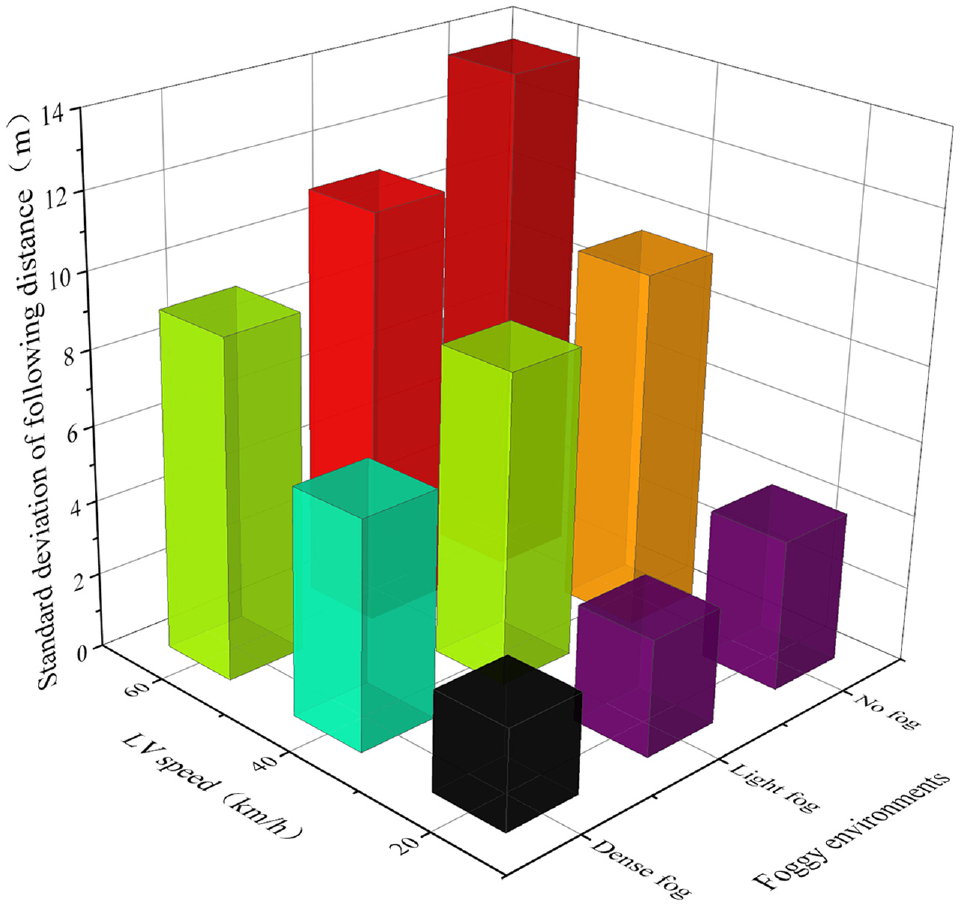
Standard deviation of the following distance.

A three-way ANOVA for driving experience, gender, and visibility showed that none of the three-factor interactions and the interaction between the two of three factors had a significant effect on the SD of the following distance (all p > 0.05). The main effect analysis showed that gender was also not significant (F = 0.250 p = 0.618 > 0.05). However, the main effect of driving experience was significant (F = 6.894, p = 0.009 < 0.05), with the SD of following distance being significantly greater among novice drivers than experienced drivers, with a mean difference of approximately 1.937 m. The main effect of visibility was also significant (F = 5.476, p = 0.005 < 0.05), with larger SD for following distances in the no-fog and light-fog environments (M = 8.745 m for no fog and M = 7.434 m for light fog), and smaller SD for following distances in the dense-fog environment, with a mean value of 5.718 m.

Standard Deviation (SD) of the Vehicle’s Lateral Offset Distance

The SD of the vehicle’s lateral offset distance under the influence of different visibilities is shown in Figure 7. With the reduction of visibility, it is more difficult for the driver to keep the vehicle running laterally and stably. This is mainly because the visibility of drivers is reduced in foggy environments, the road traffic information available is reduced, and the actual operating speed is often higher than the driver’s expected, resulting in the wrong estimation of the unknown driving conditions, which can easily cause the driver to maneuver the vehicle away from the center of the lane ( 52 ). As the LV speed decreases, the SD of the vehicle’s lateral offset distance decreases, which is mainly because of the reduction of the LV operating speed and the following speed down. The pressure of the driving operation is reduced, and the lateral movement state can be better controlled, to keep it along the lane center.

Figure 7.

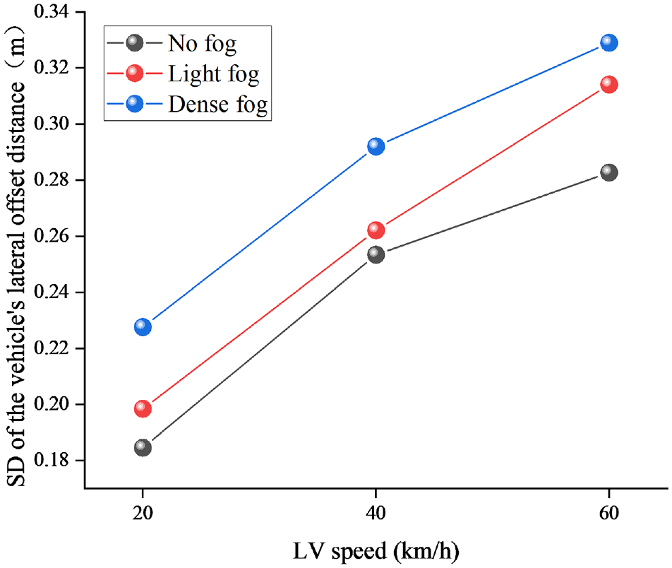
Standard deviation (SD) of the vehicle’s lateral offset distance.

According to the three-way ANOVA of visibility, driving experience, and gender, the interaction between the three factors and the interaction between the two of three factors had no significant effect on the SD of vehicle lateral offset distance (all p > 0.05). The main effect of driver gender was also not significant (F = 0.001, p = 0.972 > 0.05). However, the main effect of visibility was significant (F = 2.076, p = 0.127 < 0.05), with the SD of vehicle lateral offset distance increasing significantly as the visibility decreased. The main effect of driving experience was also significant (F = 8.815, p = 0.003 < 0.05); novices’ SD of vehicle lateral offset distance was significantly greater than that of experienced drivers.

Quantitative Analysis of Driver-Following-Behavior Risk in Different Visibility Levels

Factor Analysis Method

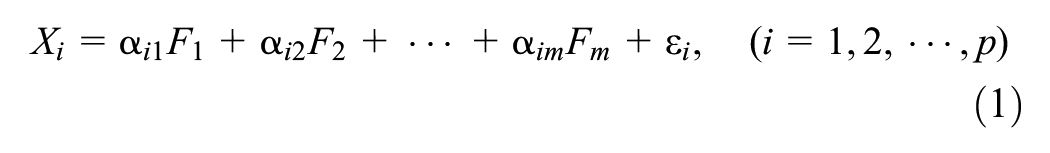
Factor analysis uses the idea of dimensionality reduction, explores the correlation coefficient matrix between variables, and divides variables with high correlation into a group, and each group of variables can be represented by a data basic structure. New variables representing the basic structure of each data group are called principal factors; thus, the number of variables is reduced. Principal factors only include most of the information of many original variables, and some information cannot be explained by principal factors, that is, special factors of the corresponding original variables. Let the random vector x = (x₁, x₂, …, x_p). The general form of the factor model is shown in Equation 1:

X_{i} = α_{i 1} F_{1} + α_{i 2} F_{2} + \dots + α_{im} F_{m} + ε_{i}, (i = 1, 2, \dots, p)

(1)

where

F ₁, F₂…F_m = a principal factor,

ε_i = a special factor, representing influencing factors other than the principal factor, m≤p.

The matrix form of the factor model is shown in Equation 2:

X = AF + ε

(2)

where

X = [\begin{matrix} X_{1} \\ X_{2} \\ ⋮ \\ X_{P} \end{matrix}], A = [\begin{matrix} α_{11} & α_{12} & \dots & α_{1 m} \\ α_{21} & α_{22} & \dots & α_{2 m} \\ \dots & \dots & \dots & \dots \\ α_{p 1} & α_{p 2} & \dots & α_{pm} \end{matrix}], F = [\begin{matrix} F_{1} \\ F_{2} \\ ⋮ \\ F_{P} \end{matrix}], ε = [\begin{matrix} ε_{1} \\ ε_{2} \\ ⋮ \\ ε_{P} \end{matrix}]

(3)

The matrix A is a factor load matrix, and the load of the ith variable on j factors is expressed by the coefficient α_ij, which reflects the importance of the ith variable X_i to the jth principal factor F_j.

There are many commonly used estimation methods for factor load matrices. Based on the previous application, the principal component analysis method is used to estimate the factor load matrix. Let λ₁≥λ₂≥…≥λ_p be the eigenvalue of the sample correlation coefficient matrix R, and let η₁,η₂,…,η_p be the corresponding standard orthogonalized eigenvector, then the principal component factor analysis load matrix A of the sample correlation coefficient matrix R is Equation 4:

A = (\sqrt{λ_{1}} η_{1}, \sqrt{λ_{2}} η_{2}, \dots, \sqrt{λ_{m}} η_{m})

(4)

The common degree of variables represents the degree of information contained in each variable explained by a common factor. The value ranges from 0 to 1. The more information of the variable explained by a principal factor, the greater its value.

By rotating the factor load matrix, the relationship between the original index variable and the principal factors can be better highlighted, so that the load of the principal factors on some original index variables is significantly larger, which is conducive to the interpretation of the actual meaning of the principal factors.

In the research, the importance of principal factors can be evaluated according to the variance contribution rate of each principal factor. In the factor load matrix A, the sum of squares of each column element α_j is denoted by $g_{j}^{2}$ , which is:

g_{j}^{2} = \sum_{j = 1}^{k} α_{ij}^{2} (i = 1, 2, \dots, p)

(5)

The factor score is obtained by calculating the relationship between the original variable and the factor. This score can be used to evaluate the score of each case on the principal factor, reflecting the information of the original variable. The factor score has two functions: one is to replace the original variable for analysis and the second is to conduct comprehensive scoring. The comprehensive score is mainly calculated based on the proportion of variance contribution rate corresponding to each common factor.

Quantitative Analysis of Driver-Following-Behavior Risk

Vehicle speed, headway, and following distance and its SD are all longitudinal behavioral indicators describing the process of driving, and the SD of vehicle lateral offset distance is an indicator describing the transverse behavior. It is found through the statistical analysis of each indicator that the trend of the indicator changes with the visibility has a relative consistency. To simplify the characterization parameters of the following behavior and further comparative analysis of the differential changes under the influence of visibility, a quantitative model of the following risk was constructed using factor analysis ( 53 ).

Firstly, the Z-score normalization method is used to eliminate the differences between different dimensions of the indicators. According to the risk trend of driving behavior reflected by the characteristics of the indicators, it can be seen that the smaller the index value of the following distance and the headway, the greater the collision risk of the following behavior. The smaller the indicator values of speed, SD of the vehicle’s lateral offset distance, and SD of following distance, the smaller the riskiness. To facilitate the comparative analysis, the index values of the following distance and headway are taken as the inverse, that is, the changing trend of all the index values is unified with the riskiness of the car following, and the smaller the values of all the indexes are, the smaller the car-following behavior riskiness.

The results of Spearman’s correlation analysis are shown in Table 1, and it can be seen that there is a strong correlation between the indicators; the results of the Kaiser-Meyer-Olkin (KMO) test and Bartlett test of sphericity show that the KMO test is 0.557, and the statistic P-value of the Bartlett test of sphericity is less than the significance level of 0.05, which applies to the factor analysis method.

Table 1.

Spearman’s Correlation Analysis

	Speed	SD of following distance	Headway	Following distance	SD of vehicle lateral offset distance
Speed	1.000	0.610^*	−0.017	−0.686^*	0.313^*
SD of following distance	0.610^*	1.000	−0.455^*	−0.741^*	0.389^*
Headway	−0.017	−0.455^*	1.000	0.579^*	−0.226^*
Following distance	−0.686^*	−0.741^*	0.579^*	1.000	−0.384^*
SD of vehicle lateral offset distance	0.313^*	0.389^*	−0.226^*	−0.384^*	1.000

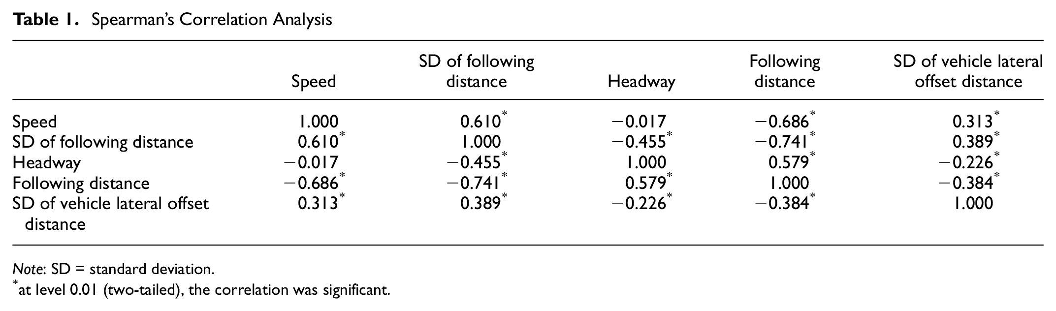
Note: SD = standard deviation.

at level 0.01 (two-tailed), the correlation was significant.

With the increase in the number of principal components, the cumulative contribution rate of principal components increases, but the increase rate tends to be slow. The initial eigenvalue of the first principal component factor F₁ is 2.636, and the contribution rate is 47.316%. The initial eigenvalue of the second principal component factor F₂ is 1.067, and the contribution rate is 26.750%. As shown in Table 2, the first two factors with eigenvalues greater than 1 were selected as the main factors, and the cumulative contribution rate of the two factors was 74.066%, which can reflect the overall information of the original variables more comprehensively.

Table 2.

Total Variance Interpretation

Composition	Initial eigenvalue			Extract the sum of squares of the load			Rotating load sum of squares
Composition	Total	Percentage of variance	Cumulative %	Total	Percentage of variance	Cumulative %	Total	Percentage of variance	Cumulative %
1	2.636	52.726	52.726	2.636	52.726	52.726	2.366	47.316	47.316
2	1.067	21.340	74.066	1.067	21.340	74.066	1.337	26.750	74.066
3	0.783	15.661	89.727	NA	NA	NA	NA	NA	NA
4	0.367	7.347	97.073	NA	NA	NA	NA	NA	NA
5	0.146	2.927	100.000	NA	NA	NA	NA	NA	NA

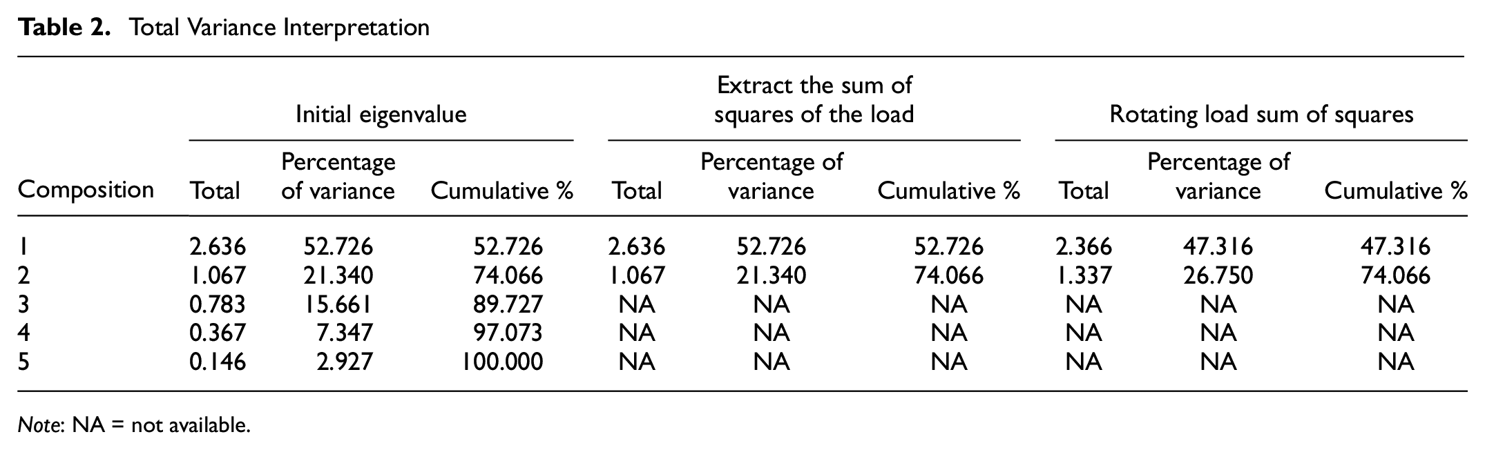
Note: NA = not available.

To further analyze the original variable information explained by the principal factor, the principal factor is rotated, as shown in Table 3. After rotation, it is found that factor 1 is related to the vehicle speed, the SD of vehicle lateral offset distance, and the following distance and its SD. Therefore, factor 1 is called the longitudinal running stability factor. Factor 2 is related to the headway, and is called the risk factor.

Table 3.

Factor Loading Matrix

Indicator	Principal factor
Indicator	F₁	F₂
Speed	0.924	0.209
SD of following distance	0.739	−0.406
Headway	−0.099	0.976
Following distance	−0.803	0.403
SD of vehicle lateral offset distance	0.558	−0.118

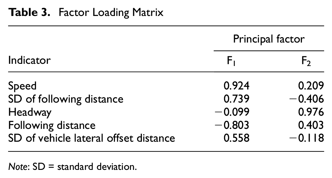
Note: SD = standard deviation.

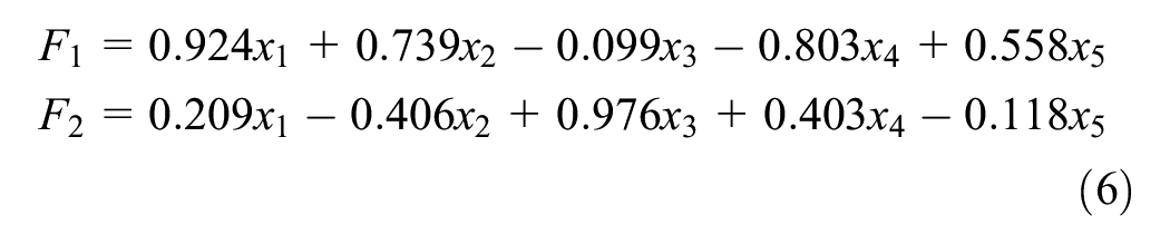
From the matrix of component score coefficients, the expressions of F₁ and F₂ as shown in Equation 6 are obtained:

\begin{matrix} F_{1} = 0.924 x_{1} + 0.739 x_{2} - 0.099 x_{3} - 0.803 x_{4} + 0.558 x_{5} \\ F_{2} = 0.209 x_{1} - 0.406 x_{2} + 0.976 x_{3} + 0.403 x_{4} - 0.118 x_{5} \end{matrix}

(6)

where

x₁ = speed,

x₂ = SD of following distance,

x₃ = headway,

x₄ = following distance, and

x₅ = SD of vehicle lateral offset distance.

The quantitative model of driver-following risk is obtained by taking the corresponding variance contribution rates of each factor as weights and unitizing the weights based on the sum of the variance contribution rates, as shown in Equation 7:

M = \frac{1}{74.066} (47.316 \times F_{1} + 26.750 \times F_{2})

(7)

To facilitate comparison, the max-min method was used to standardize the index values based on the results of factor analysis. According to the driver characteristics, the risk curve under different visibilities is drawn. According to the point plot of different genders’ risk under the influence of visibility, as shown in Figure 8a, it can be seen that, in foggy conditions, the following risk of female drivers is greater than that of male drivers; that is, female show a higher risk tendency of collision than males.

Figure 8.

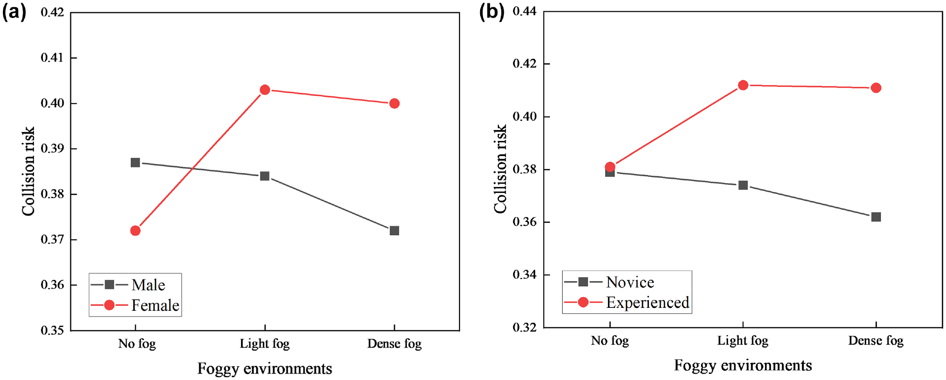
The influence of (a) driver gender and (b) driving experience on the following risk under different visibilities.

The dot-line diagram of differently experienced drivers following risk under the influence of visibility shown in Figure 8b. It can be seen that the following risk of experienced drivers is greater than that of novice drivers as visibility decreases, indicating that experienced drivers tend to keep the LV in the visual range and maintain a closer following distance, even if this increases the collision risk. However, novices drive more cautiously, and the drivers’ sense of crisis increases significantly with the reduction of visibility and they tend to keep a lower risk ( 50 ).

The results are shown in Figure 9 that the driver’s risk is the highest when driving in a light-fog environment, which is because, as visibility decreases, the driver is more cautious in driving and focuses more on controlling the vehicle to run smoothly. However, in light-fog environments, the driving psychology is more relaxed, but visibility is reduced by the foggy weather, which leads to a higher collision risk.

Figure 9.

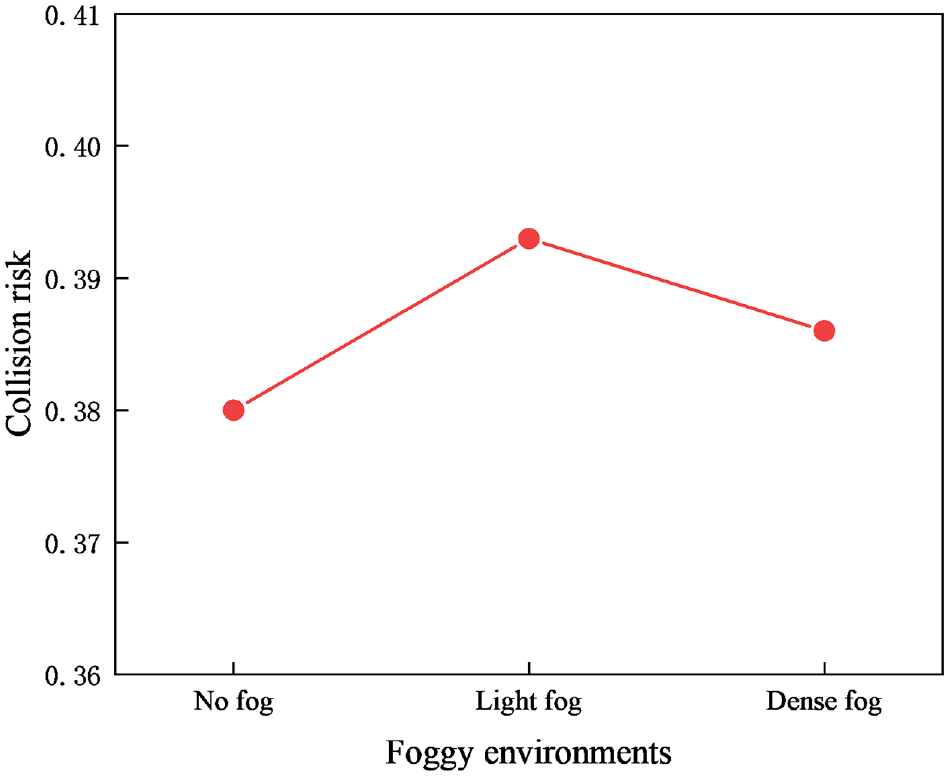
Car-following risk under different visibilities.

In summary, visibility has a significant effect on drivers’ behaviors; as visibility decreases, drivers’ following behaviors become more cautious, and the stability of vehicle longitudinal operation increases, but the visibility decrease leads to a higher risk of rear-end collision and a decrease in the control of the vehicle’s lateral movement. Drivers’ following risk is greatest in light-fog environments.

Behavioral Characterization of Drivers’ Avoidance Responses in Different Visibility Environments

Drivers’ Avoidance Responses

Braking Response Time

In this study, the braking reaction time is taken as the time interval between the appearance of the LV braking light and the driver’s braking response. A three-way ANOVA was used to explore the effects of driver gender, driving experience, and visibility on braking reaction time, and the results showed that none of the three-factor interactions, nor the interaction between the two of three factors, had a significant effect on braking reaction time (all p > 0.05). However, the main effect of visibility was significant (p = 0.001 < 0.01) and, as the fog concentration increased, the drivers’ braking reaction time increased, which is consistent with the results of previous studies ( 54 ). This is because of the increase in braking reaction time as a result of the driver’s vision being interfered with fog, insensitivity to the surrounding driving environment, and reduced ability to perceive LV speed changes.

The main effect of driving experience was also significant (p = 0.016 < 0.01), and the braking reaction time of novice drivers was significantly greater than that of experienced drivers, with a mean difference of 0.382 s, which was consistent with previous studies ( 55 ). Whereas the gender main effect was not significant (p = 0.322 > 0.05), the mean braking reaction time of male drivers was 0.156 s faster than that of females, which is similar to previous studies ( 56 ). This may be because the height of female drivers is generally shorter than that of men. When they are driving, their vision field is smaller because they sit lower, which affects their reaction time in judging the LV running state. In addition, if it is the case that female drivers are more nervous when driving on foggy days, this may interfere with their cognitive ability to LV brake state, resulting in prolonged braking reaction time.

Following Distance

Multivariate ANOVA was used to explore the effects of gender, driving experience, and visibility on following distance. The results showed that the interaction between three factors and the two of three factors had no significant effects on the following distance (all p > 0.05). The main effect of gender was not significant (F = 1.811, p = 0.180 > 0.05), but the following distance of males was greater than that of female drivers, and the mean difference was 2.645 m. This may be because males are more cautious when driving in foggy conditions and maintain a larger following distance. Once the LV brakes, the male driver has a shorter reaction time and can brake more quickly to prevent collisions.

The main effect of driving experience was significant (F = 7.685, p = 0.006 < 0.01), and the following distance of the novice drivers was significantly greater than that of the experienced drivers, with an average difference of 5.448 m. That is, novice drivers braked at a greater relative distance from the LV. Novice drivers may be more cautious, to ensure safety, and keep a large following distance with the front car when driving. The main effect of visibility was significant (F = 5.056, p = 0.077 < 0.01) and, with the decrease of visibility, the mean following distance decreased.

Speed

Under the collision and conflict scenario caused by the LV braking, the instantaneous speed of the rear vehicle at the braking time was collected. The results of multivariate ANOVA showed that the interaction of visibility, gender, and driving experience, the interaction between the two of three factors, and the single of three factor main effect had no significant influence on the speed (all p > 0.05).

Headway

Headway combines the following distance and speed, which can reflect the safety when following a vehicle in a more comprehensive way. The headway was analyzed when the LV braked and the rear driver reacted to the braking during the car-following process with different visibilities, and a three-way ANOVA was used to investigate the effects of gender, driving experience, and visibility on the headway, which showed that the interaction of the three factors and the interaction of the two of three factors did not have a significant effect on the headway (all p > 0.05). The main effect analysis showed that gender also had no significant effect on headway (F = 2.524, p = 0.114 > 0.05). However, visibility had a significant effect on headway (F = 3.366, p = 0.037 > 0.05) and, as the fog concentration increased, the headway decreased. Firstly, the decrease in visibility reduced the visual stimulus of the surrounding environment to the driver, which can easily lead to the driver’s wrong judgment of the LV speed, thus increasing the tendency to shorten the following distance. Secondly, the driver tends to keep the LV in sight and, thus, the traveling speed is closer to the LV speed. These two factors lead to a tendency for drivers to maintain a smaller headway when traveling in low-visibility conditions. The main effect of driving experience was also significant (F = 5.921, p = 0.016 < 0.05), with novices having significantly greater headway than experienced drivers, with a mean difference of 0.448 s.

Maximum Brake Depth

Under different foggy environments and driving conditions, the maximum braking depth taken by the rear vehicle driver was analyzed when the LV decelerated leading to a collision conflict. In this study, the braking depth is taken to be the normalized braking depth, that is, the ratio of the braking force generated by the brake pedal to the maximum braking force, with a range of values of [0,1]. A value of 0 denotes no braking input, and 1 denotes full braking.

The effects of driving experience, gender, and visibility and their interaction on drivers’ maximum braking depth were further explored using the multifactor ANOVA method, which showed that the interaction of the three factors did not have a significant effect on maximum braking depth (p = 0.931 > 0.05). Further analysis of the interaction between the two of three factors revealed that the interaction of driving experience and gender had a significant effect on maximum braking depth (p = 0.014 < 0.05).

Firstly, the effect of driving experience on maximum braking depth was considered under different genders, and the results of a main effects test for driving experience showed that the maximum braking depth of male experienced drivers was greater than that of male novice drivers, with a mean difference of 0.072. Maximum brake depth was significantly greater for female experienced drivers than for female novice drivers, with a mean difference of 0.225. This is because, compared with the novice, experienced drivers have more driving experience. The collision risk of avoidance operation behavior in the brain to establish a power stereotype, when aware of the risk of collision conflict, tends to lead to a greater depth of braking as soon as possible to reduce speed, to avoid rear-end collision.

Further analyzing the effect of gender on maximum braking depth among differently experienced drivers, a main effects test for gender showed that maximum braking depth was greater for male novice drivers than for female novice drivers, with a mean difference of 0.009, but not significantly different (p > 0.05). Among experienced drivers, female drivers had significantly greater maximum braking depth than males (p < 0.05), with a mean difference of 0.145, which may be because females tend to take more aggressive braking measures in collision conflict scenarios.

There was a significant main effect of visibility (p = 0.005 < 0.01) with an increase in fog concentration; the maximum braking depth increased (no fog M = 0.403, light fog M = 0.485, dense fog M = 0.525). The main effect of driving experience was also significant (p < 0.01), and the maximum braking depth of novice drivers was significantly smaller than that of experienced drivers, with a mean difference of 0.149. The main effect of gender was also significant (p = 0.029 < 0.05), with the maximum braking depth of male drivers being significantly smaller than that of females, with a mean difference of 0.068.

Vehicle Collision Conflict Risk

In the analysis of vehicle collision risk, time to collision (TTC) is often used as a measure of the emergency degree of collision risk. The smaller the TTC value, the higher the collision risk and the greater the collision possibility. The higher the TTC value, the lower the collision risk and the lower the collision possibility.

A multifactorial ANOVA was used to explore the effects of driving experience, gender, and visibility on TTC values, and it was found that there was no significant effect of the three-factor interaction and the interaction between the two of three factors on the TTC values (all p > 0.05). There was a significant main effect of visibility (F = 6.312, p = 0.002 < 0.05), and the mean TTC values decreased significantly with increasing fog concentration (no fog TTC = 7.097 s, light fog TTC = 6.506 s, and dense fog TTC = 5.754 s), suggesting that drivers have a greater likelihood of collision when they are following a vehicle in a lower-visibility environment. However, the main effect of driving experience was not significant (F = 2.188, p = 0.596 > 0.05), whereas the novice TTC mean (6.223 s) was smaller than that of experienced drivers (6.681 s), which may be because experienced drivers can maintain a safer follow-through traveling condition, thus avoiding collisions. The gender main effect was also not significant (F = 0.928, p = 0.337 > 0.05). The mean TTC for male drivers (6.303 s) was smaller than that of females (6.601 s), indicating that male drivers take relatively more risk with regard to collision risk at the moment of braking. However, the mean TTC value of male drivers at the moment of braking was still greater than 5.5 s. According to research, the risk of collision is lower for TTC values ≥5.5 s ( 57 ). Therefore, females are more cautious in maneuvering their vehicles to follow during driving compared with male drivers.

A Comprehensive Analysis of Driver Braking Response Characteristics in Different Visibility Levels

The combined effects of visibility, speed, and following distance at the moment of LV braking on the driver’s braking reaction time were further investigated. The drivers experienced three driving scenarios with different visibilities, and each scenario experienced two collision conflict situations caused by LV braking, at the same time, taking into account that there may be a stronger correlation between the variables. Therefore, with the help of a linear mixed model, the driver is regarded as a random effect, and the differences in individual behaviors are fully considered to explore the comprehensive effects of fog concentration, speed, and the following distance at the LV braking time on the drivers’ braking reaction time ( 58 ).

The linear mixed model is an extension of the simple linear model; whereas the traditional general linear model independent variables are fixed effects, the linear mixed model introduces random effects on this basis, incorporating some non-independent properties of the sample into the model, allowing for both fixed and random effects, and is particularly suitable for situations where the data are not independent. Its basic form is shown in Equation 8:

Y_{ij} = β + α_{j} + \sum_{h = 1}^{p} β_{h} X_{hij} + ε_{ij}

(8)

where

Y_ij = the measured value of driver j in the i response variable,

X_hij = the ith value of the hth independent variable at the location of driver j,

β = the intercept,

β_h = the regression coefficient of the hth independent variable,

α_j = the individual difference of driver j, which follows a normal distribution of mean 0 and variance G, and

ε_ij = the random error of the ith value of driver j, subject to a normal distribution with mean 0 and variance R.

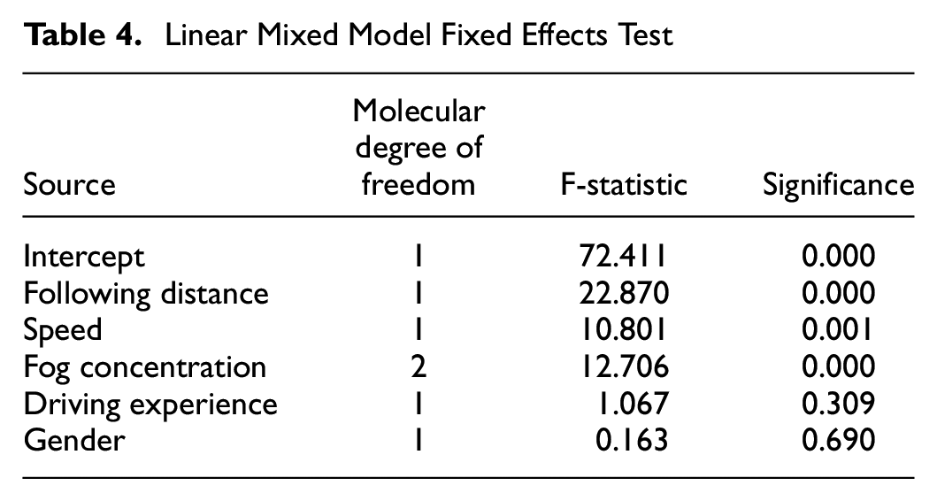
A driver braking reaction time prediction model was constructed with driving experience, gender, fog concentration, vehicle speed, and following distance, where the vehicle speed is the instantaneous speed of the vehicle maneuvered by the driver at the moment of LV braking, and following distance is the distance between LV and following vehicle at the moment of LV braking. The fixed effect test results of the linear mixed model are shown in Table 4. At the confidence level of p = 0.05, following distance, vehicle speed, and fog concentration all have significant effects on the braking reaction time (all p < 0.05). Driver gender (p = 0.690 > 0.05) and driving experience (p = 0.447 > 0.05) had no significant effects on braking reaction time.

Table 4.

Linear Mixed Model Fixed Effects Test

Source	Molecular degree of freedom	F-statistic	Significance
Intercept	1	72.411	0.000
Following distance	1	22.870	0.000
Speed	1	10.801	0.001
Fog concentration	2	12.706	0.000
Driving experience	1	1.067	0.309
Gender	1	0.163	0.690

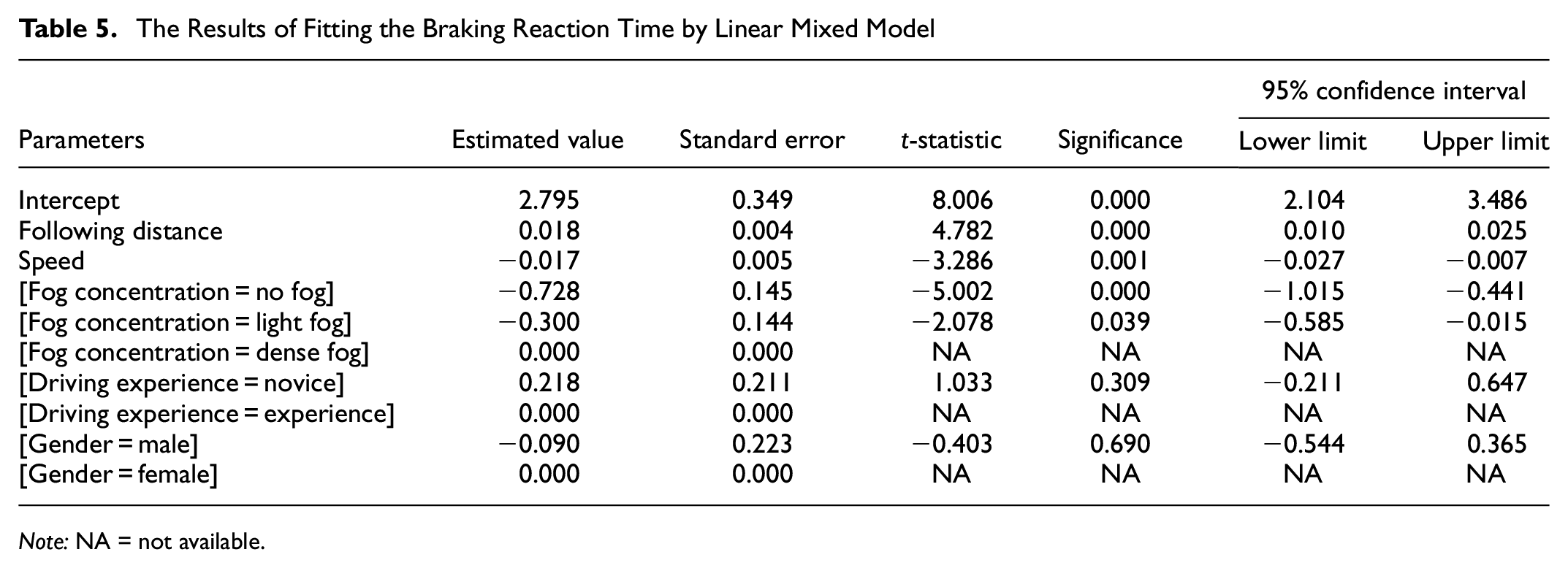
The linear mixed model regression results are shown in Table 5, and show that the effect of a dense fog environment on braking reaction time is positive compared with no-fog (p < 0.01) and light-fog (p = 0.039 < 0.05) environments under car-following conditions. With the increase of fog concentration, the drivers’ braking reaction time increased, that is, the decrease of visibility increased the drivers’ braking reaction time. At the same time, the drivers’ braking reaction time decreases with the increase of driving speed and increases with the following distance increase when the LV brakes.

Table 5.

The Results of Fitting the Braking Reaction Time by Linear Mixed Model

Parameters	Estimated value	Standard error	t-statistic	Significance	95% confidence interval
Parameters	Estimated value	Standard error	t-statistic	Significance	Lower limit	Upper limit
Intercept	2.795	0.349	8.006	0.000	2.104	3.486
Following distance	0.018	0.004	4.782	0.000	0.010	0.025
Speed	−0.017	0.005	−3.286	0.001	−0.027	−0.007
[Fog concentration = no fog]	−0.728	0.145	−5.002	0.000	−1.015	−0.441
[Fog concentration = light fog]	−0.300	0.144	−2.078	0.039	−0.585	−0.015
[Fog concentration = dense fog]	0.000	0.000	NA	NA	NA	NA
[Driving experience = novice]	0.218	0.211	1.033	0.309	−0.211	0.647
[Driving experience = experience]	0.000	0.000	NA	NA	NA	NA
[Gender = male]	−0.090	0.223	−0.403	0.690	−0.544	0.365
[Gender = female]	0.000	0.000	NA	NA	NA	NA

Note: NA = not available.

Limitation

In future studies, the number of participants in the test can be increased, the characteristics of driving behavior can be further analyzed, and the mechanism of drivers’ following behavior change under the influence of visibility can be more deeply explored by combining the analysis of drivers’ physiological and psychological characteristics. There was a gender imbalance among the drivers recruited for this study. An equal number of drivers of different genders could be recruited for further studies. In this study, the sequence of scene tests was randomly selected. However, the random sequence has the risk of uneven distribution of scenes across participants, which may lead to learning effects and bias in the results; this can be solved by using Latin Square designs.

Conclusions

In this study, the driving simulator method was used to construct the scenarios of car following and emergency braking of the LV. The effects of driving environments with different visibilities, driver gender, and driving age on car-following behavior were explored. The main findings are as follows:

1) This study further confirms that, when driving in a foggy environment, the driver’s behavior changes significantly. Some drivers adopt a conservative following strategy; to ensure driving safety, they actively reduce the speed and give up following the LV, allowing it to drive out of sight ( 59 ).

2) In the car-following environment, drivers tend to maintain a smaller following distance and headway with the reduction of visibility. By keeping the LV within the view field, the SD of the following distance decreases with the reduction of visibility. In the lateral motion state of the vehicle, the SD of vehicle lateral offset distance increases with the decrease of visibility, and decreases with the decrease of following speed. These results show that drivers are more careful to maintain a stable operation speed under a dense-fog environment; the SD of the vehicle speed is minimum and the SD of the following distance is reduced. The quantitative model analysis of vehicle-following risk based on factor analysis shows that the rear-end collision risk of experienced drivers is higher than that of novice drivers, and the risk of female drivers is higher than that of male drivers. Driving in fog increases risk, but driving in light fog results in higher risk.

3) In the scenario of rear-end collision risk caused by LV emergency braking in a foggy environment, the drivers’ braking reaction time increases with the increase of fog concentration and is significantly affected by driving experience. The braking reaction time of novice drivers is greater than that of experienced drivers, and there is no significant difference in gender. The speed, following distance, and headway of emergency braking time change according to the same law as the stable car-following state; the maximum braking depth increases with the decrease of visibility. Reduced visibility increases the risk of rear-end collision. As the visibility decreases, the braking reaction time increases, and the driver’s collision risk at the braking time increases. The braking reaction time of the driver decreases with the increase of the driving speed and increases with the increase of the following distance when the LV brakes.

4) The results of this study are of great significance to the formulation of traffic management and control measures under the influence of visibility, provide a reference for the targeted training of driving behavior in adverse weather, and provide a research method and a systematic experimental analysis method for the influence of other intervening factors on driving behavior.

Footnotes

Author Contributions

The authors confirm contribution to the paper as follows: study conception and design: T. Wei, T. Zhu; data collection: T. Wei; analysis and interpretation of results: T. Wei, H. Bai, L. Zhao, X. Wang; draft manuscript preparation: T. Wei, H. Bai. All authors reviewed the results and approved the final version of the manuscript.

Declaration of Conflicting Interests

The author(s) declared no potential conflicts of interest with respect to the research, authorship, and/or publication of this article.

Funding

The author(s) disclosed receipt of the following financial support for the research, authorship, and/or publication of this article: This work was supported by the Scientific Research Foundation of Shandong Jiaotong University (Grant No. Z202314), Shandong Jiaotong University Talent Introduction Research Start-up Fund (Grant No. BS2023035), the Inovative Team Project of Ji'nan Government (Grant No. 202333036), National Key R&D Program of China (Grant No. 2019YFE0108000), Research on the new architecture and key technologies of hybrid enhanced intelligent “traffic brain” (Grant No. 2021TSGC1011), Research on the new architecture and key technologies of hybrid enhanced artificial intelligence “traffic brain”(Grant No. 202160101683), and data-driven integrated guidance and collaborative control of urban expressway traffic (Grant No. 202250101842).

Ethical Approval

This study was approved by the Ethics Committee of Chang’an University, Xi’an, China.

ORCID iD

Tianzheng Wei

Data Accessibility Statement

Data will be made available from the corresponding author on request.

References

Keay

Simmonds

The Association of Rainfall and Other Weather Variables with Road Traffic Volume in Melbourne, Australia. Accident Analysis & Prevention, Vol. 37, No. 1, 2005, pp. 109–124.

Cools

Moons

Wets

Assessing the Impact of Weather on Traffic Intensity. Weather, Climate, and Society, Vol. 2, No. 1, 2010, pp. 60–68.

Theofilatos

Yannis

A Review of the Effect of Traffic and Weather Characteristics on Road Safety. Accident Analysis & Prevention, Vol. 72, 2014, pp. 244–256.

Cheng

Wang

Liu

Bai

Investigating the Severity of Expressway Crash Based on the Random Parameter Logit Model Accounting for Unobserved Heterogeneity. Advances in Mechanical Engineering, Vol. 13, No. 12, 2021, p. 16878140211067278.

Kenk

M. A.

Hassaballah

DAWN: Vehicle Detection in Adverse Weather Nature Dataset. arXiv preprint arXiv:200805402, 2020.

Awal

Mushfiq

M. M.

Al Islam

A. A.

Fault Tolerance Analysis of Car-Following Models for Autonomous Vehicles. IEEE Transactions on Intelligent Transportation Systems, Vol. 23, No. 11, 2022, pp. 20036–20045.

Yadav

Redhu

Driver’s Attention Effect in Car-Following Model with Passing Under V2V Environment. Nonlinear Dynamics, Vol. 111, No. 14, 2023, pp. 1–17.

Zhou

Longitudinal Car-Following Control Strategy Integrating Predictive Collision Risk. Applied Mathematical Modelling, Vol. 121, 2023, pp. 1–20.

Yang

H. H.

Peng

Development of an Errorable Car-Following Driver Model. Vehicle System Dynamics Vol. 48, No. 6, 2010, pp. 751–773.

10.

Naing

Cai

Nan

Tiantian

Liang

Dynamic Data-Driven Microscopic Traffic Simulation using Jointly Trained Physics-guided Long Short-Term Memory. ACM Transactions on Modeling and Computer Simulation, Vol. 32, No. 4, 2022, pp. 1–27.

11.

Kim

Lovell

D. J.

Kim

Empirical Results of Effects of Various Causal Factors on Car-Following Behavior. Transportation Research Record: Journal of the Transportation Research Board, 2010. 2188: 174–186.

12.

Zhang

Jin

P. J.

McQuade

S. T.

Piccoli

A Review on Longitudinal Car-Following Model. arXiv preprint arXiv:230407143, 2023.

13.

A. W.

Chan

A. H.

The Effects of Driver Factors and Sign Design Features on the Comprehensibility of Traffic Signs. Journal of Safety Research, Vol. 39, No. 3, 2008, pp. 321–328.

14.

Musk

L. F.

Climate as a Factor in the Planning and Design of New Roads and Motorways. In Highway Meteorology (A. H. Perry and L. J. Symons, eds.), CRC Press, London, 1991, pp. 1–26.

15.

Liu

Zhao

Wang

Research on Driving Obstacle Detection Technology in Foggy Weather Based on GCANet and Feature Fusion Training. Sensors, Vol. 23, No. 5, 2023, p. 2822.

16.

Abdel-Aty

Cai

Lee

Park

Developing an Algorithm to Assess the Rear-End Collision Risk Under Fog Conditions Using Real-Time Data. Transportation Research Part C: Emerging Technologies, Vol. 87, 2018, pp. 11–25.

17.

Reinolsmann

Alhajyaseen

Brijs

Pirdavani

Hussain

Brijs

Sandstorm Animations on Rural Expressways: The Impact of Variable Message Sign Strategies on Driver Behavior in Low Visibility Conditions. Transportation Research Part F: Traffic Psychology and Behaviour, Vol. 78, 2021, pp. 308–325.

18.

Rittger

Schmidt

Maag

Kiesel

Driving Behaviour at Traffic Light Intersections. Cognition, Technology & Work, Vol. 17, 2015, pp. 593–605.

19.

Hoogendoorn

R. G.

Tamminga

Hoogendoorn

S. P.

Daamen

, eds. Longitudinal Driving Behavior Under Adverse Weather Conditions: Adaptation Effects, Model Performance and Freeway Capacity in Case of Fog. In: 13th International IEEE Conference on Intelligent Transportation Systems, IEEE, Funchal, Portugal, 2010, pp. 450–455.

20.

Xuguang

Jianping

Research on the Fixation Transition Behavior of Drivers on Expressway in Foggy Environment. Safety Science, Vol. 119, 2019, pp. 70–75.

21.

Peng

Abdel-Aty

Shi

Assessing the Impact of Reduced Visibility on Traffic Crash Risk Using Microscopic Data and Surrogate Safety Measures. Transportation Research Part C: Emerging Technologies, Vol. 74, 2017, pp. 295–305.

22.

Abdel-Aty

Wang

Rahman

M. S.

Combined Connected Vehicles and Variable Speed Limit Strategies to Reduce Rear-End Crash Risk Under Fog Conditions. Journal of Intelligent Transportation Systems, Vol. 24, No. 5, 2020, pp. 494–513.

23.

Wang

Liang

Evans

Fatal Crashes Involving Large Numbers of Vehicles and Weather. Journal of Safety Research, Vol. 63, 2017, pp. 1–7.

24.

Chen

K.- P.

Hsiung

P.- A.

Vehicle Collision Prediction Under Reduced Visibility Conditions. Sensors Vol. 18, No. 9, 2018, p. 3026.

25.

Moore

R. L., and L.

Cooper. Fog and Road Traffic. Transport and Road Research Laboratory TRRL Report LR 446, TRRL, Crowthorne. 1972.

26.

Abdel-Aty

Ekram

A. -A.

Huang

Choi

A Study on Crashes Related to Visibility Obstruction Due to Fog and Smoke. Accident Analysis & Prevention, Vol. 43, No. 5, 2011, pp. 1730–1737.

27.

Brooks

J. O.

Crisler

M. C.

Klein

Goodenough

Beeco

R. W.

Guirl

Tyler

P. J.

, et al. Speed Choice and Driving Performance in Simulated Foggy Conditions. Accident Analysis & Prevention, Vol. 43, No. 3, 2011, pp. 698–705.

28.

Van Der Horst

Hogema

Time-to-Collision and Collision Avoidance Systems, Proc., 6th Int. Co-Operation on Theories and Concepts in Traffic Safety (ICTCT) Workshop, FACTUM and ICTCT, Vienna, Austria, 1994, pp. 59–66.

29.

Shi

Tan

Effect Analysis of Intermittent Release Measures in Heavy Fog Weather with an Improved CA Model. Discrete Dynamics in Nature and Society, 2013, p. 812562.

30.

Liu

Yang

Zhen

Modeling and Simulation of Car Following in Fog Based on Cellular Automata. Journal of System Simulation, Vol. 33, No. 10, 2021, pp. 2399–2410.

31.

Gao

Shi

Effect of Low-Visibility in Haze Weather Condition on Longitudinal Driving Behavior in Different Car Following Stages. Journal of Jilin University (Engineering), Vol. 47, No. 6, 2017, pp. 1716–1727.

32.

Kang

J. J.

Andersen

G. J.

Effects of Reduced Visibility from Fog on Car-Following Performance. Transportation Research Record: Journal of the Transportation Research Board, 2008. 2069: 9–15.

33.

Huang

Yan

Duan

Rakotonirainy

Gao

Improving Car-Following Model to Capture Unobserved Driver Heterogeneity and Following Distance Features in Fog Condition. Transportmetrica A: Transport Science, Vol. 20, No. 1, 2022, pp. 1–24.

34.

Abdel-Aty

Lee

Crash Risk Analysis During Fog Conditions Using Real-Time Traffic Data. Accident Analysis & Prevention, Vol. 114, 2018, pp. 4–11.

35.

MacGill

Reframing Cognitive Behaviour Theory from a Systems Perspective. Systemic Practice and Action Research, Vol. 31, No. 5, 2018, pp. 495–507.

36.

Mueller

A. S.

Trick

L. M.

Driving in Fog: The Effects of Driving Experience and Visibility on Speed Compensation and Hazard Avoidance. Accident Analysis & Prevention, Vol. 48, 2012, pp. 72–79.

37.

Lee

Guldmann

J.-M.

von Rabenau

Impact of Driver’s Age and Gender, Built Environment, and Road Conditions on Crash Severity: A Logit Modeling Approach. International Journal of Environmental Research and Public Health, Vol. 20, No. 3, 2023, p. 2338.

38.

Al-Ghamdi

A. S.

Experimental Evaluation of Fog Warning System. Accident Analysis & Prevention, Vol. 39, No. 6, 2007, pp. 1065–1072.

39.

Trick

L. M.

Lochner

Toxopeus

Wilson

, eds. Manipulating Drive Characteristics to Study the Effects of Mental Load on Older and Younger Drivers. Driving Assessment Conference, University of Iowa, Canada, 2009.

40.

Kang

J. J.

Andersen

G. J.

Age-Related Declines in Car Following Performance Under Simulated Fog Conditions. Accident Analysis & Prevention, Vol. 42, No. 3, 2010, pp. 818–826.

41.

Pavlou

Christodoulou

Yannis

The Impact of Weather Conditions and Driver Characteristics on Road Safety on Rural Roads. Transportation Research Procedia, Vol. 72, 2023, pp. 4081–4088.

42.

Johnson

M. J.

Chahal

Stinchcombe

Mullen

Weaver

Bédard

Physiological Responses to Simulated and On-Road Driving. International Journal of Psychophysiology, Vol. 81, No. 3, 2011, pp. 203–208.

43.

Underwood

Crundall

Chapman

Driving Simulator Validation with Hazard Perception. Transportation Research Part F: Traffic Psychology and Behaviour, Vol. 14, No. 6, 2011, pp. 435–446.

44.

Lizama

L. E. C.

Arvin

Verschueren

S. M.

Van Dieën

J. H.

Assessing Age-Related Balance Deterioration: Visual or Mechanical Tasks?

Clinical Biomechanics, Vol. 65, 2019, pp. 116–122.

45.

Zhao

Wan

Research on Influence of Emotion on Novice Drivers’ Visual Characteristics. China Safety Science Journal, Vol. 32, No. 12022, p. 34.

46.

Horswill

M. S.

Taylor

Newnam

Wetton

Hill

Even Highly Experienced Drivers Benefit from a Brief Hazard Perception Training Intervention. Accident Analysis & Prevention, Vol. 52, 2013, pp. 100–110.

47.

Smith

S. S.

Horswill

M. S.

Chambers

Wetton

Hazard Perception in Novice and Experienced Drivers: The Effects of Sleepiness. Accident Analysis & Prevention, Vol. 41, No. 4, 2009, pp. 729–733.

48.

Lochrane

T. W.

Al-Deek

Dailey

D. J.

Krause

Modeling Driver Behavior in Work and Nonwork Zones: Multidimensional Psychophysical Car-Following Framework. Transportation Research Record: Journal of the Transportation Research Board, 2015. 2490: 116–126.

49.

Hammit

B. E.

Ghasemzadeh

Ahmed

M. M.

Young

R. K.

Evaluation of Weather-Related Freeway Car-Following Behavior Using the SHRP 2 Naturalistic Driving Study, Transportation Research Board 97th Annual Meeting, Washington, D.C., 2018.

50.

Saffarian

Happee

Winter

J. d.

Why Do Drivers Maintain Short Headways in Fog? A Driving-Simulator Study Evaluating Feeling of Risk and Lateral Control During Automated and Manual Car Following. Ergonomics, Vol. 55, No, 9, 2012, pp. 971–985.

51.

Nengchao

Jinjin

Weifeng

Yugang

Classification of Driving Style Using Simplified Features of Headway Under the Connected Vehicles Environment. Journal of Transport Information and Safety, Vol. 40, No. 1, 2022, pp. 116–125.

52.

Snowden

R. J.

Stimpson

Ruddle

R. A.

Speed Perception Fogs Up as Visibility Drops. Nature, Vol. 392, No. 6675, 1998, p. 450.

53.

Brandenburg

Oehl

Hartwig

Driving Anger Expression in Germany—Validation of the Driving Anger Expression Inventory for German Drivers. Traffic Injury Prevention, Vol. 20, No. 1, 2019, pp. 52–57.

54.

Gao

Sun

Sze

Song

Shi

Impacts of Reduced Visibility Under Hazy Weather Condition on Collision Risk and Car-Following Behavior: Implications for Traffic Control and Management. International Journal of Sustainable Transportation, Vol. 14, No. 8, 2020, pp. 635–642.

55.

Chen

Cao

Logan

D. B.

Investigation into the Effect of an Intersection Crash Warning System on Driving Performance in a Simulator. Traffic Injury Prevention, Vol. 15, No. 5, 2011, pp. 529–537.

56.

Dickerson

A. E.

Reistetter

T. A.

Burhans

Apple

Typical Brake Reaction Times Across the Life Span. Occupational Therapy in Health Care, Vol. 30, No. 2, 2016, pp. 115–123.

57.

Jin

Van Arem

Yang

van der Mascha

Martijn

Safety Lane Change Model of Vehicle Assistant Driving on Highway. Journal of Jilin University (Engineering and Technology Edition), Vol. 39, No. 3, 2009, pp. 582–586.

58.

Möls

Constraints on Random Effects and Mixed Linear Model Predictions. Acta Applicandae Mathematica, Vol. 79, 2003, pp. 17–23.

59.

Broughton

K. L.

Switzer

Scott

Car Following Decisions Under Three Visibility Conditions and Two Speeds Tested with a Driving Simulator. Accident Analysis & Prevention, Vol. 39, No. 1, 2007, pp. 106–116.