
Abstract
Map matching is the process of matching global positioning system (GPS) trajectory data with map data. Its purpose is to determine the actual route of the moving object. Because of factors such as positioning devices and the environment, the GPS trajectory data obtained may not be accurate. In location-based services, map matching can be used to address the accuracy and reliability issues of GPS location data. There are currently many map-matching algorithms, for example, spatio-temporal-based (STD) matching algorithm, improved interactive voting-based map-matching (IIVMM) algorithm, and turning-point-based (TPB) offline map-matching algorithm, but existing algorithms have some shortcomings, such as low matching accuracy on complex roads or low sampling rates, and routing calculation time bottlenecks. Therefore, this paper proposes a fast matching algorithm based on constrained value pruning that is suitable for complex roads. The algorithm considers the multi-directional features within the road and uses secondary calculations to determine candidate points, improving the accuracy of candidate point selection. Additionally, two pruning strategies based on constrained values are introduced to reduce the majority of the routing calculation process and improve the matching efficiency. Finally, comparative experiments are conducted on a real trajectory dataset. The results show that, compared with STD, IIVMM, and TPB algorithms, the algorithm accuracy is improved by about 2% to 4%, and the running time is reduced by about 30%.
Map matching is the process of matching global positioning system (GPS) trajectory data with map data to determine the actual position and movement trajectory of vehicles or pedestrians on the road network. Because of the effects of multipath, environmental noise, and low-power design on the mobile receiver module, GPS positioning technology has a low trajectory sampling rate and large positioning error, and cannot be used directly. Map matching can project the initial positioning point onto the actual road, complete the missing trajectory, and minimize the deviation of the moving target from the road.
With the rapid development of mobile internet and the Internet of Things, vehicles equipped with positioning modules generate massive trajectory data. Researchers are committed to quickly and effectively obtaining traffic information from these data and further applying them to many location-based services (LBS), such as map services, traffic management, and route searching. LBS services and map matching are closely related because LBS relies on location data to provide services, while map matching is the process of matching location data with map data to determine their accurate position. Map matching is a necessary preprocessing step for trajectory data and has strong practical application value for LBS.
Given a road network
A sample of candidate point set of global positioning system point
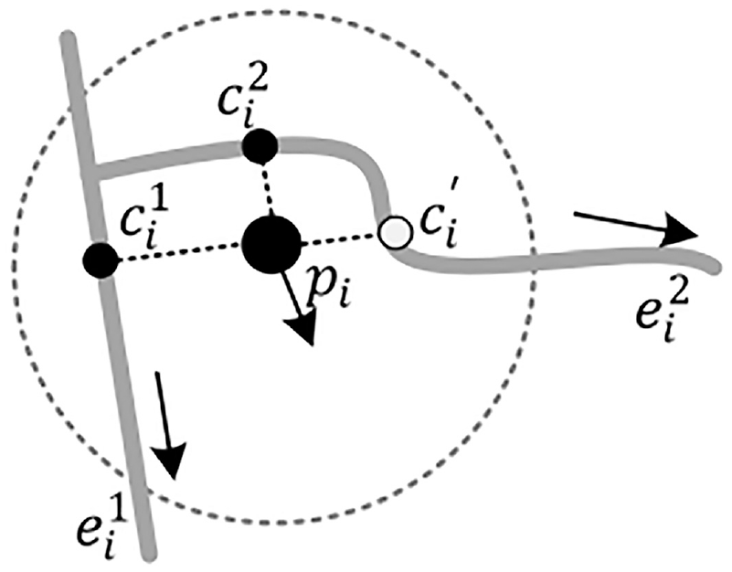
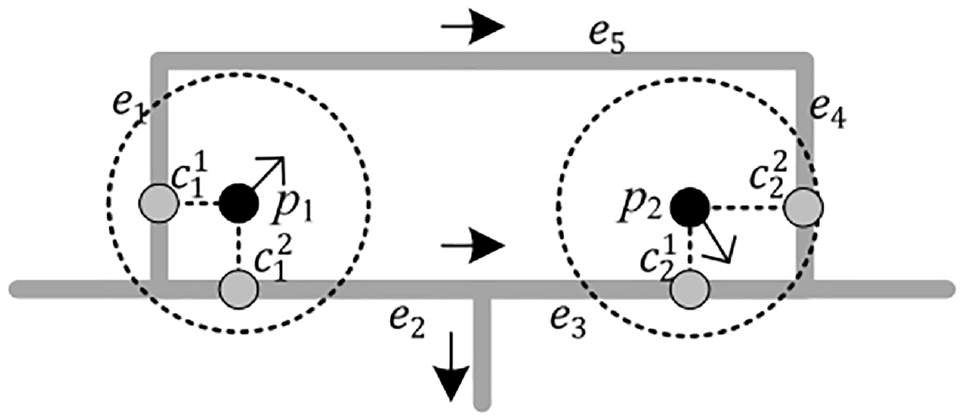
In addition, complex road networks and computational time pose challenges common to the development of all novel algorithms. Complex roads generate an abundance of potential matching points, which can potentially result in incorrect path matches—an issue that will be elaborated on in subsequent sections. Furthermore, the dataset utilized in this paper comprises taxi trajectories. Typically, taxi trajectory data are gathered from the intricate urban road systems, where complexity is inherent. Existing HMM-based matching algorithms incorporate a variety of feature factors for calculation, which improves the matching accuracy. However, there are still some shortcomings in such algorithms. First, the internal direction change of the road section is not considered in the candidate set selection stage, resulting in the calculated observation probability not being accurate: as in Figure 1, the projection point
To alleviate the limitations brought by the above problems, this paper is dedicated to improving the accuracy and computational efficiency of the map-matching algorithm from two aspects that have been neglected by related studies. In summary, the main contributions of this paper are as follows:
1) For map matching under complex roads, the algorithm in this paper considers the distance and direction factors in the candidate point extraction stage and uses the road midpoint information to determine the candidate points by secondary computation, thus improving the matching accuracy.
2) For the problem of excessive computation time cost, a fast matching strategy based on limited value pruning is proposed, and an improved Dijkstra (IDijkstra) routefinding algorithm is proposed, which reduces the unnecessary routing computation process and greatly improves the efficiency of matching.
In conclusion, extensive experiments were conducted on real data sets by combining contribution points 1 and 2, and the experimental results show that the matching accuracy of Pruning Features Map Matching (PFMM) for GPS trajectories can reach 92.6%. Comparing the algorithm of this paper with three existing methods, the performance of the proposed PFMM algorithm outperforms the three existing algorithms at both high and low sampling frequencies, the running time is reduced by more than 30% compared with the three existing algorithms, and the matching efficiency is greatly improved.
Related Work
Map matching is the process of corresponding trajectory data to road networks. The concept was first proposed by Tanaka et al. and has evolved from simple search methods to complex and accurate route matching ( 3 ). Map-matching algorithms can be classified into local matching algorithms and global matching algorithms based on the range of track inputs. Local matching algorithms use only some of the current trajectory points to calculate the partial solution, which gives a faster computation speed and is suitable for processing real-time and streaming trajectory data to provide support for some real-time services, such as vehicle navigation and driving route prediction. Local matching algorithms are more suitable for processing high sampling rate trajectory data, and the effectiveness of the algorithm will be reduced for low sampling rate trajectory data. Global matching algorithms, on the other hand, process the stored complete trajectory data and find the best matching route in the road network, which can satisfy some trajectory-based services, such as travel route recommendation, cab abnormal trajectory detection, and so forth. Since the conversion and storage of raw data will be burdensome and that there is equipment battery limitation, which usually reduces the sampling rate of trajectory data, how to perform map matching based on low sampling GPS trajectories is an important problem, which has been better solved in recent years’ map-matching algorithm research.
Simple Map-Matching Algorithms
Early simple map-matching algorithms could return vertices or edges that were close in geometry or topology and trajectory distance, generating matching results. Geometry-based map-matching algorithms include point-to-point matching, point-to-line matching, and line-to-line matching (4–6). These methods are relatively simple to implement, but the algorithmic computation is large, and they are greatly affected by trajectory noise and sparsity. Topology-based map-matching mainly relies on the topology of the road network and considers vehicle historical data and road topology to determine the vehicle’s position (7–9). The weighted topology matching method in Quddus et al. considers different types of data such as position, speed, direction, and travel time to improve matching accuracy ( 9 ). However, it is still susceptible to GPS trajectory noise and sparse roads, and is not suitable for complex road networks.
The key to a simple map-matching algorithm is how to measure distance similarity. The most commonly used distance function is the Frechet distance, which is suitable for measuring curve similarity with spatial temporal sequence, but is sensitive to trajectory outliers ( 5 ). The longest common subsequence (LCSS) is an alternative method to Frechet distance which considers the similar parts between trajectories as a measure of similarity and skips trajectory points that exceed a threshold value because of matching distance. These features make it robust to noise. Cui et al. proposed an improved LCSS, known as the Longest common subsequence with heading penalty (LCSS-HP) method, which incorporates direction label information for trajectory segments and allows candidate road segments to be matched with multiple consecutive GPS points, further improving accuracy ( 10 ).
Advanced Map-Matching Algorithms
Advanced map-matching algorithms refer to those that use Kalman filtering, fuzzy logic, Bayesian inference, conditional random fields (CRF), HMM, and neural networks, among others (1, 2, 11–29). Advanced map-matching algorithms often consider more comprehensive information, resulting in higher accuracy.
CRF is the interaction between observations, using characteristic functions to more freely express the relationship between states. The map-matching algorithm in reference, which applies to low sampling trajectories, applies GPS point candidate points and paths to a CRF model, and finds the best matching candidate points through a forward-backward recursive algorithm. The map-matching algorithm proposed by Hunter et al. combines the observation model and the driver model into a CRF to obtain the most probable trajectory ( 20 ). The map-matching algorithm based on CRF normalizes the global observation sequence and adds all possible candidate paths to the calculation, resulting in a huge search space and low efficiency.
HMM is one of the most widely used methods. HMM can be used to model sequential data of vehicle driving trajectories and calculate transition probabilities by comparing factors such as distance and direction between GPS points and road segments on the road network. It can utilize contextual information, whereby the current observation value is not only influenced by the current state, but also by previous states, and use dynamic programming based on the
The HMM-based algorithm uses projection once to determine candidate points in the candidate point selection stage, without considering the internal curvature of road segments, which may lead to inaccuracies in some cases. In addition, the large amount of routing calculation required for global matching in such algorithms leads to high computational costs.
In addition, some research results are based on Bayesian rules to perform iterative prediction and update on current matching results. Taguchi et al. proposed a matching method based on a probabilistic path prediction model ( 12 ). The algorithm is based on a Bayesian network observation model and a route prediction model to match GPS trajectory data with a map road network. The route prediction model generates a candidate set of routes, and the observation model is used to calculate the matching probability for each route and select the best matching route. Hao et al. ( 31 ) proposed an improved Kalman filter and GPS error correction method, which uses historical flight paths and road map information to update the Kalman filter state vector and related parameters ( 19 ). The Kalman filter can predict future states based on current states and measurements. During the modeling process, the white noise assumption of the Kalman filter theory was considered, and the incremental error between two adjacent points was modeled as an approximation of Gaussian error and then incorporated into the Kalman filter.
Fuzzy logic can score matching candidate objects and select the candidate object with the highest score function value as the matching result. Quddus et al. proposed a high-precision map-matching algorithm based on fuzzy logic ( 13 ). This algorithm first calculates candidate routes based on vehicle sensor data, and uses fuzzy logic to score the routes, ultimately determining the best matching route. In recent years, neural networks have been increasingly applied to map matching problems. Neural networks combine multiple neurons in a nonlinear manner to calculate the score of candidate paths, and encoder-decoder frameworks are used to map trajectories to corresponding paths. Jin et al. ( 32 ) proposed a map-matching model based on deep learning ( 12 ). They constructed a transformer-based map-matching model using transfer learning methods, generated trajectory data for pre-training the transformer model, and then fine-tuned the model using real data to minimize model development costs and reduce the gap between real and virtual. The average Hamming distance of three metrics at the point and segment levels was used to evaluate model performance using F-score and Bilingual Evaluation Understudy (BLEU), using the transformer’s attention weight to draw the map matching process, and finding out how the model correctly matches road segments. Neural-network-based models are sensitive to data size and, without sufficient data, they may fall into overfitting. These models heavily rely on the traffic patterns behind the training data, and different cities may have different numbers of roads and driving patterns. Therefore, models trained for one city cannot be directly applied to another city.
In addition, map-matching methods based on deep learning include Feng et al. who build a “trajectory2road” model with attention mechanism to map the sparse and noisy trajectory into the accurate road network based on the “seq2seq” learning framework ( 25 ). Jiang et al. propose a general and robust deep learning-based model, Learning TO Map Matching (L2MM), to tackle these issues ( 26 ). First, high-quality representations of low-quality trajectories are learned by two representation enhancement methods, that is, enhancement with high-frequency trajectories and enhancement with the data distribution. Second, to embrace more heuristic clues, typical mobility patterns are recognized in the latent space and further incorporated into the map-matching task. Finally, based on the available representations and patterns, a mapping from trajectories to corresponding paths is constructed through a joint optimization method. Liu et al. present GraphMM, a graph-based approach that exploits the graph nature of map matching and incorporates graph neural networks and conditional models to leverage both road and trajectory graph topology, while managing to align road segments and trajectories in latent space ( 27 ). We formally analyze the expressive power of our model in capturing various correlations and propose efficient algorithms for model training and inference.
This paper proposes a fast matching algorithm based on HMM. This algorithm takes into account the multi-directional characteristics of road networks and employs supplementary calculations to identify candidate points, thereby enhancing the precision of their selection. Moreover, a fast matching algorithm utilizing bounded value pruning, PFMM, is introduced, which significantly curtails the computational demands of route processing, thus boosting the overall matching efficiency.
Problem Definition
Given an initial GPS coordinate point and a digital vector map, the goal of map matching is to find the path the vehicle is most likely to travel on the map. In this paper, map matching based on HMM is studied.
In this section, we give the definition of the map matching problem. First, we give some basic definitions of map matching, and then we give relevant definitions of candidate set and candidate path probability in specific matching.
A GPS point
A GPS trajectory
A road network can be viewed as a directed graph
A subsegment
A route is a set of consecutive sections starting at
The map-matching problem is defined as follows. Given the road network
Candidate Set Preparation
Data Preprocessing
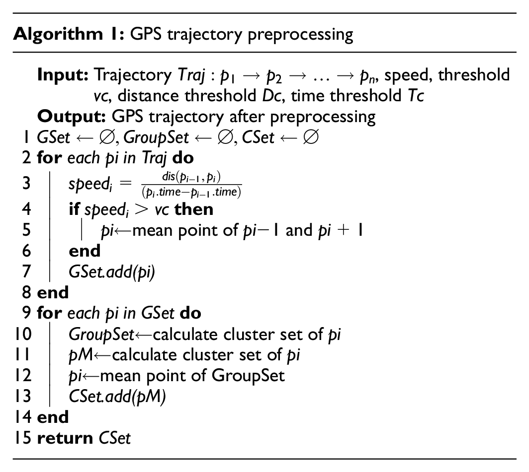
In this section, data pre-processing is performed before the map-matching algorithm is executed, with the purpose of analyzing and filtering the raw data for outlier filtering and dwell point detection for GPS trajectories, to filter out the data that are not valuable in the raw data, as well as those that may interfere with the results. Data preprocessing pseudocode is shown in Algorithm 1, and the specific process is as follows.
Outlier Filtering Strategy
Outliers are a few GPS points that are abnormal to the normal data. These points are often abrupt to ensure the accuracy of the algorithm and need to remove the track outliers. The outlier filtering strategy is described below.
1) Specify the speed threshold (
2) If
3) If
Take Figure 2 as an example, showing part of the trajectory
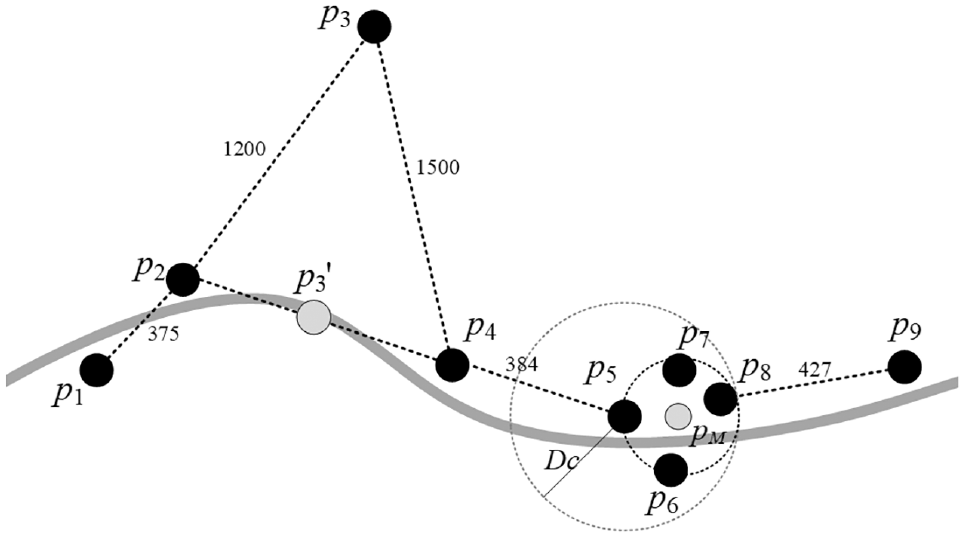
Examples of outliers and dwell points.
Dwell Point Detection Strategy
The dwell point indicates the geographical location of the vehicle that stays for a period of time. When the vehicle stops at a certain location, the GPS points recorded by the positioning device are often not the same coordinates, but a series of extremely similar trajectory points, so, to reduce unnecessary computation, the aggregated GPS points are clustered.
The
1)
2)
If
As shown in Figure 2, the sampling time interval is known to be 30 s, and Dc = 200 m and Tc = 30 s are specified. When
Candidate Points Extraction
In this section, the candidate points extraction method is introduced, using a quadratic computation to extract candidate points strategy to search a set of candidate points for each GPS point before the matching calculation. Since, in real situations, there may be multiple turns inside the road and a road contains multi-directional features, the intermediate point information of the road section is considered for the first time to extract preselected points and candidate points separately.
Candidate Road Segment Extraction
For each GPS point
Preselected Points Extraction
Given a GPS point
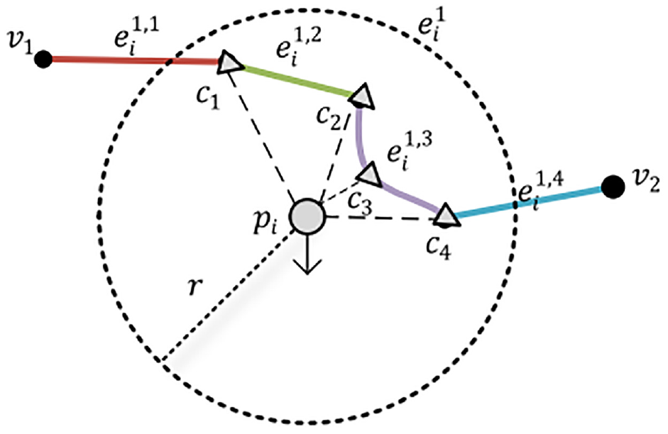
A sample of extracting preselected sets for global positioning system point p i .
The similarity between preselected points and trajectory points is measured by two criteria: distance and direction. The distance criterion is the Euclidean distance between the two points, and the direction criterion is the difference in direction between the trajectory point and the candidate point. The direction value of a preselected point is determined by the direction value of the subsegment it belongs to. The formula for calculating the direction of subsegment
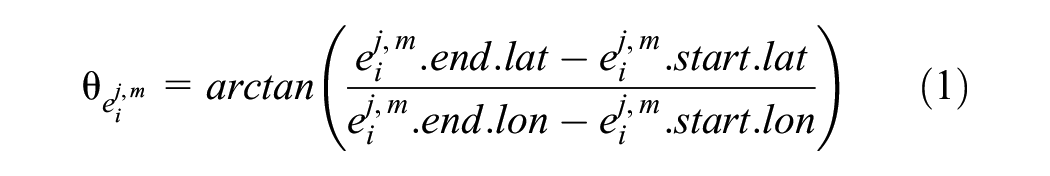
where
To reduce the error in direction calculation, we adopt an optimal range rule to assign direction values to preselected points:
1) If the preselected point itself is not an intermediate or endpoint of the road segment, the three adjacent subsegments are included in the range, and the direction closest to
2) If the preselected point is an intermediate or endpoint of the road segment, the two adjacent subsegments before and after the preselected point are included in the range, and the direction value is determined. In Figure 3, the adjacent subsegments of candidate point
The definition of the direction difference between trajectory points and preselected points is as follows:

where
Candidate Points Extraction
For a GPS point
where
The overall similarity function

For a set of preselected points
and the optimal preselected point is called the candidate point, denoted as

Candidate points are extracted for all candidate segments of each GPS point
Based on the processed underlying road network data, the end point, length, and intermediate point data of the road are extracted and stored in the form of grid index to record the information of objects falling on the grid and reduce the search time in the process of searching for candidate road segments.
Candidate Route Probability Analysis
This section introduces candidate point probability calculation, candidate route probability calculation, and candidate graph construction. After candidate set extraction, each GPS point in the trajectory can generate a set of candidate points. In this section, first, the observation probability is defined, and the probability for candidate points is analyzed and calculated. Then, considering road connectivity, transfer probability is defined, probability calculation for candidate routes is performed, and, finally, candidate graphs of trajectories are generated based on candidate points and candidate routes.
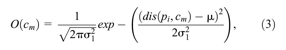
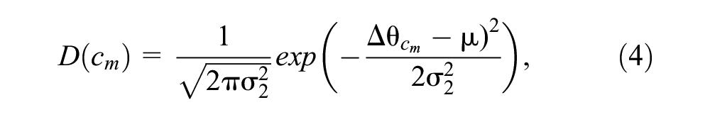
The similarity function is described as the observation probability and has the following definitions based on the distance similarity and directional similarity.
The

The larger the distance
In some cases, considering only the observation probability is likely to result in a situation where the wrong candidate point has a larger observation probability, leading to a wrong matching route. For example, in Figure 4, there are
A sample of parallel road.
A candidate route denotes a shortest route on a road network starting at
The transition probability denotes the candidate route
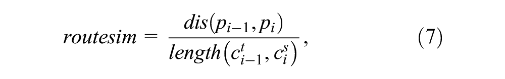
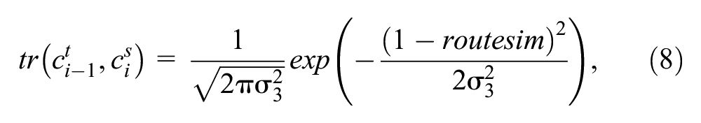
where
If the route ratio is smaller, the transition probability value is larger, and the matching probability of its candidate route is larger.
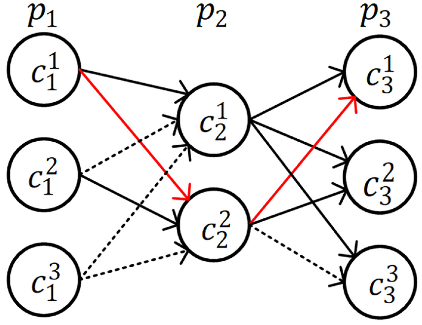
According to the candidate points and candidate routes of trajectory, the candidate graph of trajectory can be generated, and the later calculations about trajectory matching are based on the candidate graph. Figure 5 shows the candidate graph
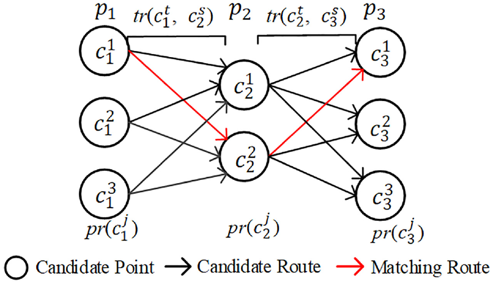
A sample of p1 →p2 →p3 candidate graph.
The candidate graph can find the final matching sequence, that is, the candidate graph contains the routes of all trajectory points of a candidate point. Since GPS points have the characteristics of time sequence, the final matching route can be calculated according to the incremental topology of the candidate graph.
Map-Matching Algorithm
Overview of Map-Matching Algorithm
According to the candidate graph definition, the cumulative probability measures the corresponding candidate route matching probability size. Figure 5 shows that, except for the
The cumulative probability
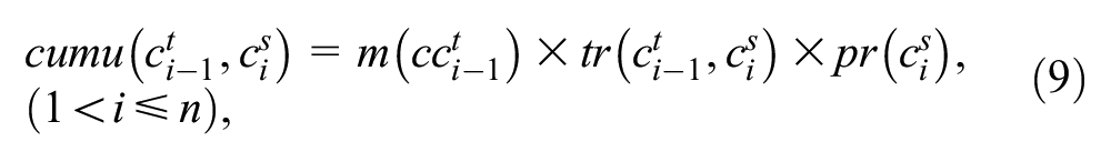
where
The optimal cumulative probability is the maximum value in
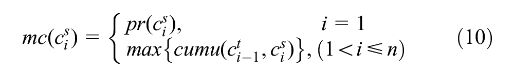
where
Table 1 shows the cumulative probabilities of all candidate routes for the trajectory
Candidate Routes of
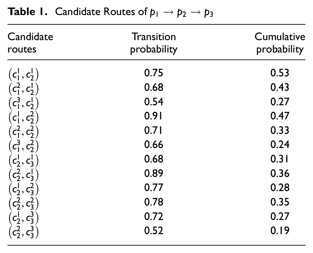
The optimal cumulative probability of candidate points at the last point
As shown in Table 1, the candidate point
The map matching process is the most time-consuming when it comes to calculating the transfer probabilities of candidate routes, as many shortest route queries have to be performed on the road network. In the traditional HMM-based map-matching algorithm, neighboring candidate points are fully connected and all transfer probabilities have to be calculated, which is very time-consuming. As shown in Table 1, the trajectory
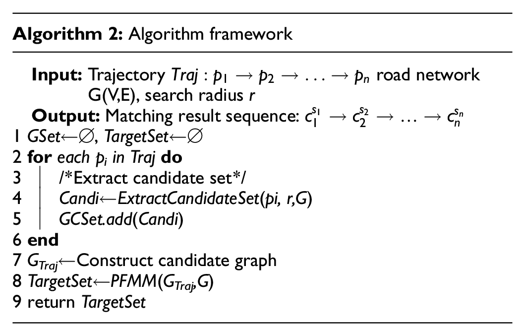
To address this computational bottleneck, this paper proposes the PFMM algorithm, which reduces most of the shortest route query process through pruning optimisation. As shown in Figure 6, the algorithm can prune four candidate routes, which can reduce part of the computational cost. The performance improvement of this algorithm is especially significant in complex dense road networks. Algorithm 2 shows the map-matching algorithm framework.
A sample of
PFMM Algorithm Process
The PFMM algorithm is able to filter a portion of unnecessary candidate route probability calculations. Its algorithm is divided into three main steps: 1) Determine the baseline candidate route for candidate points, 2) Candidate route pruning optimization, and 3) Optimal matching route recovery. Algorithm 3 shows the pseudocode of PFMM.
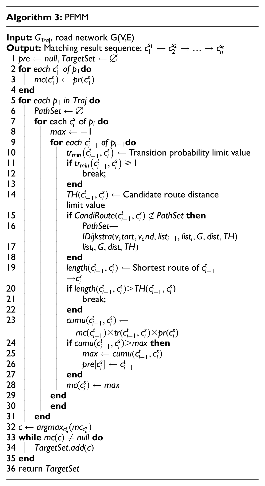
Determine the Baseline Candidate Route for Candidate Points
For each candidate point in the candidate graph for
Candidate Route Pruning Optimization
For the remaining unvisited candidate points of
In particular, for the candidate route
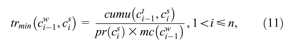
where
Pruning strategy 1 and pruning strategy 2 are proposed based on the transition probability limit values.
Pruning Strategy 1
If the transition probability is bounded to
Theorem 1: Given a candidate point
Proof: The
If the transition probability is limited to
Theorem 2: Given a candidate point and a candidate route
Proof: The current maximum cumulative probability value
To determine whether the transition probability satisfies
The candidate route distance limit is calculated as follows:
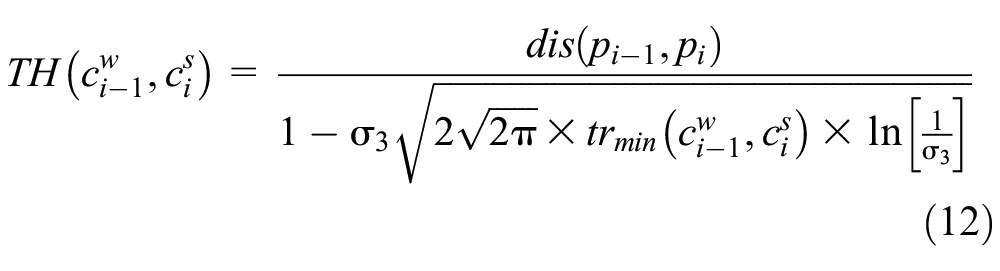
where
Pruning Strategy 2
If the transition probability limit
Theorem 3: Given a candidate point
Proof: Theorem 2 shows that
Optimal Matching Route Recovery
When the last
As shown in Table 2, the matching procedure for the
Global Matching Calculation of p1 →p2 →p3
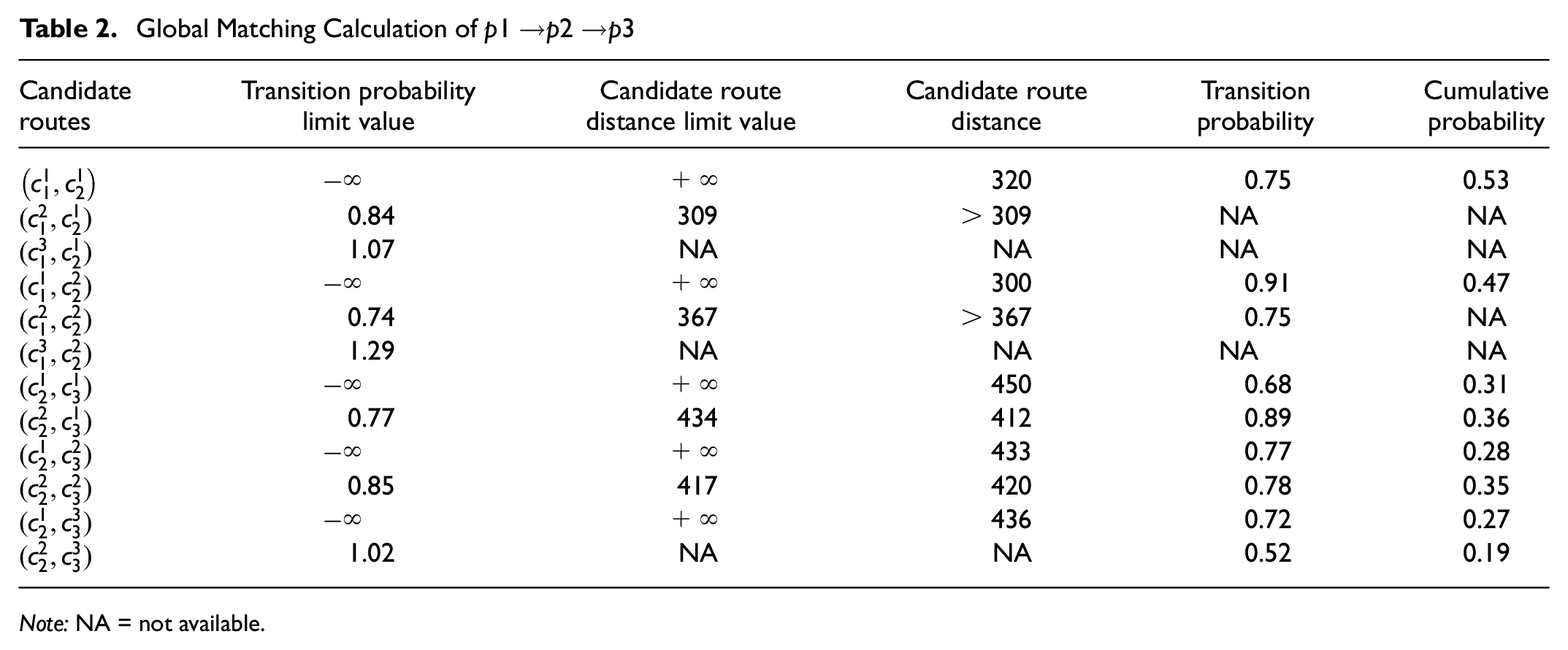
Note: NA = not available.
First, the point
Then, the point
Next, the point
The candidate point
Next, the point
At this point, the computation between
IDijkstra Algorithm
When the starting and ending points are near to each other, according to dwell point detection strategy, in data preprocessing, these points merge into a single stopping point. Furthermore, when discarding nodes, according to
This section describes the routefinding algorithm used, the IDijkstra algorithm, which minimizes the search process for the shortest route of the road network. Algorithm 4 shows the algorithm pseudocode. The basic steps of the IDijkstra algorithm are described as follows.
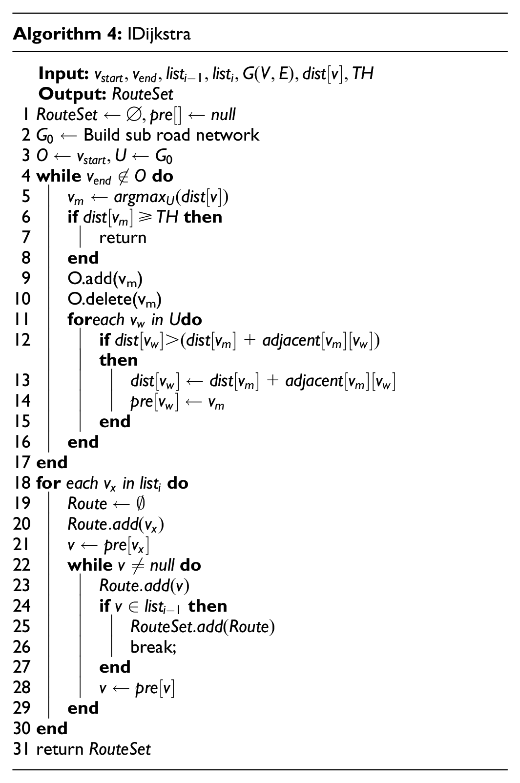
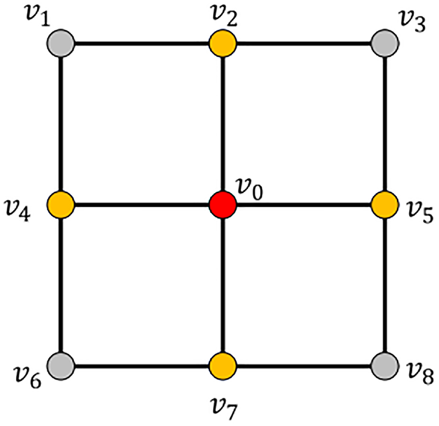
Construct the Subroad Network
Construct the subroad network according to the target starting point to limit the scope of subsequent searches, the method is described as follows:
1) Denote the target start and end point
2) To search more potential road sections, for the nodes in
3)
A sample of
Shortest Route Search
Based on the original Dijkstra algorithm process, which is calculated from the starting point of the destination, the route-finding process consists of the following three parts:
1) Introducing the sets
2) Selecting the vertex
3) Looping step 2 until the destination end point is added to the visited set; defining sets
Experiments
In this section, the PFMM algorithm in this paper is implemented in Java language and tested against the STD, IIVMM, and turning-point-based (TPB) map-matching algorithms. The experimental environment is AMD Ryzen 7 5700U CPU @ 1.80 GHz; 16 GB RAM; 1TB HDD, and Windows 10 OS.
Dataset Description
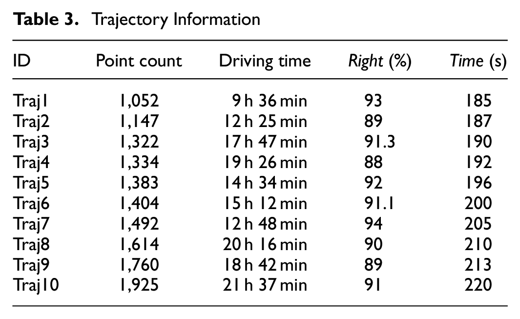
The dataset employed for this experiment consists of real-world road networks and vehicle trajectories. We utilized Shanghai, China, road network data, obtained from OpenStreetMap, which encompasses 215,070 road segments and 213,734 road nodes ( 32 ). The GPS data were sourced from the Shanghai taxi trajectory dataset provided by the Smart City Research Group at the Hong Kong University of Science and Technology. Each GPS point within this dataset carries attributes such as timestamp, longitude, latitude, direction, speed, and occupancy status. To evaluate the map-matching algorithm’s performance, we extracted 10 full-day taxi trajectories from the dataset. These trajectories collectively consist of 14,443 GPS points. Table 3 provides a summary of the trajectory information, detailing the number of GPS points in each trajectory and their corresponding travel times. A graphical representation of selected trajectory points is displayed in Figure 8.
Trajectory Information
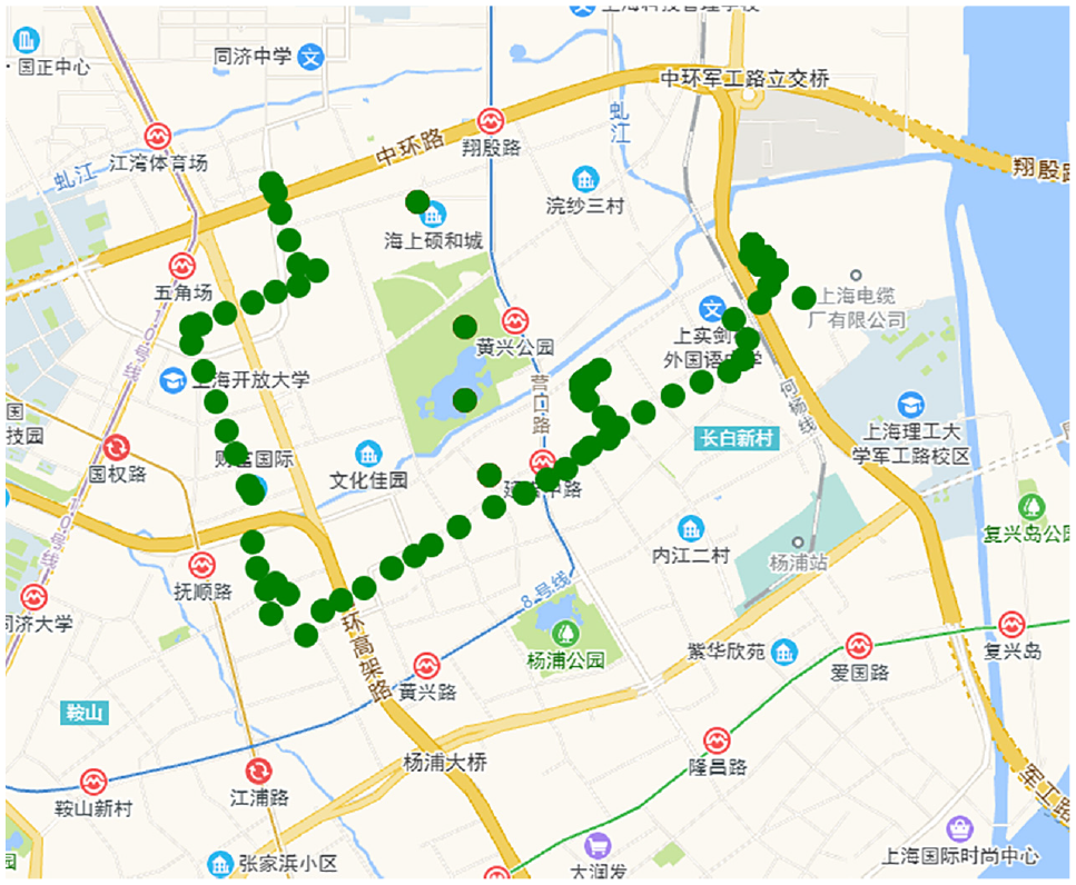
Point plot of partial global positioning system trajectory.
The real trajectories were matched using the ST algorithm and further refined manually. Experiments indicated that trajectory length has negligible impact on matching accuracy. To illustrate this, default parameter values were used, and results for matching accuracy (Right) and processing time (Time) across 10 trajectories are presented in Table 3. Specific GPS trajectory points were selected for map matching, with results depicted in Figure 9. In the figure, the red trajectory denotes unprocessed GPS points, the blue trajectory represents the GPS roadmap after preprocessing, and the green trajectory depicts the actual GPS route. It is evident from the figure that algorithm-derived trajectories closely align with the actual trajectories, exhibiting minimal errors.
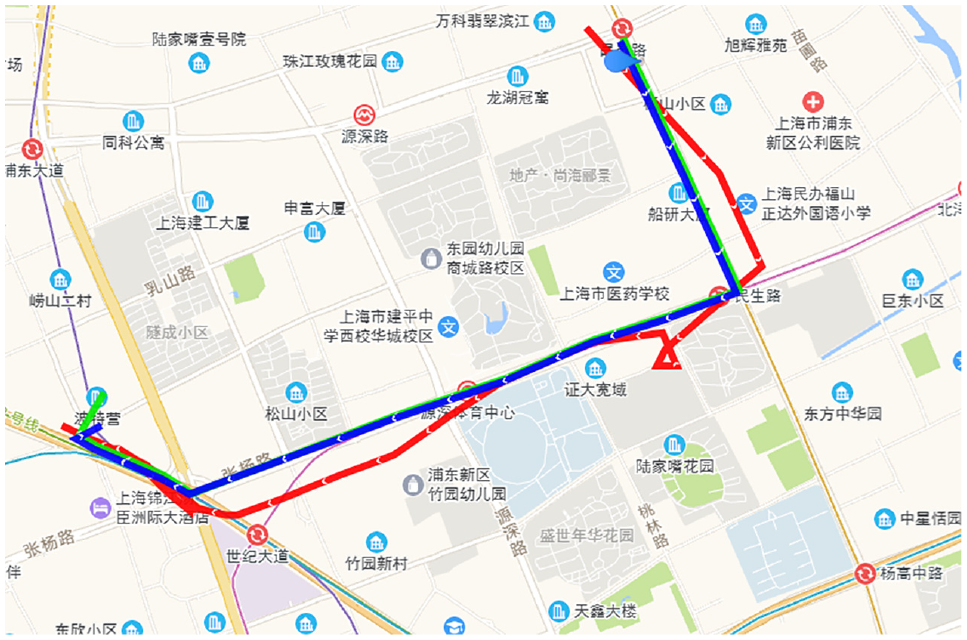
Example plot of trajectory matching.
Parameter Settings
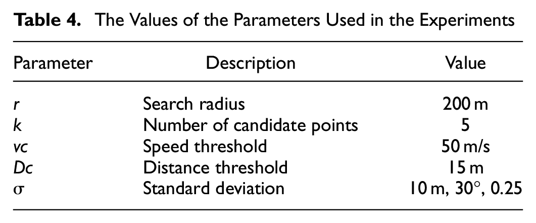
In this paper, the sampling interval of GPS points is within 10–50 s.In the trajectory pre-processing, the velocity threshold
The Values of the Parameters Used in the Experiments
In the experiments conducted for this paper, the PFMM algorithm is benchmarked against STD, IIVMM, TPB, and L2MM algorithms (1, 2, 24, 26). For the STD, IIVMM, and L2MM algorithms, the observation probability parameters are initialized to their default settings as prescribed in this work. Meanwhile, the remaining parameters for these three algorithms are fine-tuned in accordance with the specifications detailed in the pertinent literature.
Evaluation Criteria Setting
This section describes three criteria for measuring the performance of this paper and the comparison algorithm, and one for the PFMM algorithm.
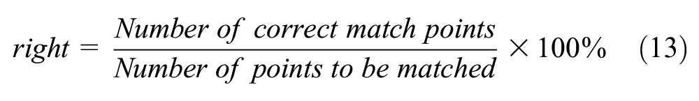
1) Percentage of correctly matched
2) Running time of the algorithm on the same platform: Time
3) The length of the matching result route: Glength
4) The number of prunings during the matching process of the PFMM algorithm: pruning
The performance of the algorithm can be measured in many aspects through the above four criteria. The first criterion, Right, is determined by the number of matched road segments, and the maximum value of Right is set to 100% in the experiment. The second standard,
Impact of Changing the Speed Threshold (vc)
In this section, the performance of the PFMM, STD, IIVMM, TPB, and L2MM algorithms under different values of vc in the trajectory preprocessing outlier filtering stage is compared (1, 2, 24, 26). In general, when the vc value is too large, it is difficult to filter outliers, while, when the vc value is too small, some normal points will be filtered, affecting the matching accuracy.
Figure 10a shows the comparison of the accuracy of the four algorithms under different vc values; on average, the accuracy of the PFMM algorithm is about 3.7% higher than that of the STD, IIVMM, and TPB algorithms (1, 2, 24). However, compared with the L2MM algorithm, the accuracy of the PFMM algorithm is about 15%. Figure 10b shows the influence of different vc values on the matching time. On average, the running time of the PFMM algorithm is reduced by about 34.1% compared with the comparison algorithms. Figure 10c shows the influence of different vc values on the matching path length; it can be seen that the matching result path length of the proposed algorithm is shorter, and the detour degree is reduced by about 2.8%. Figure 10d shows the pruning of the PFMM algorithm, where the number of prunings increases as the value of vc increases. According to the experimental results, it can be seen that, when the vc value is 50 m/s, the performance of the algorithm in all aspects is better, so the default vc value is 50 m/s in the following experiments.
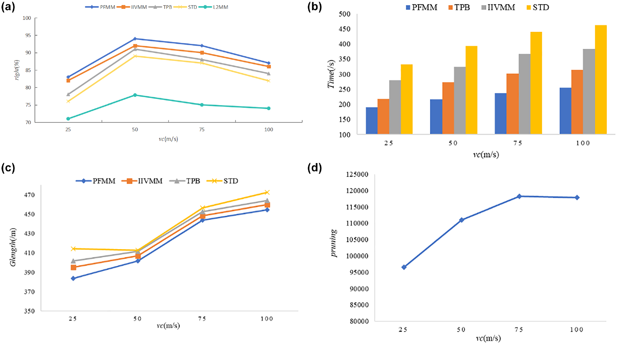
The impact of speed threshold (vc) value on algorithms: (a) The impact of speed threshold (vc) value on algorithms rights; (b) The impact of speed threshold (vc) value on algorithms Time; (c) The impact of speed threshold (vc) value on Glength; and (d) The impact of speed threshold (vc) value on pruning.
Impact of Changing the Distance Threshold (Dc)
In this section, the performance of the PFMM, STD, IIVMM, TPB, and L2MM algorithms under different values of
Figure 11a shows the influence of different
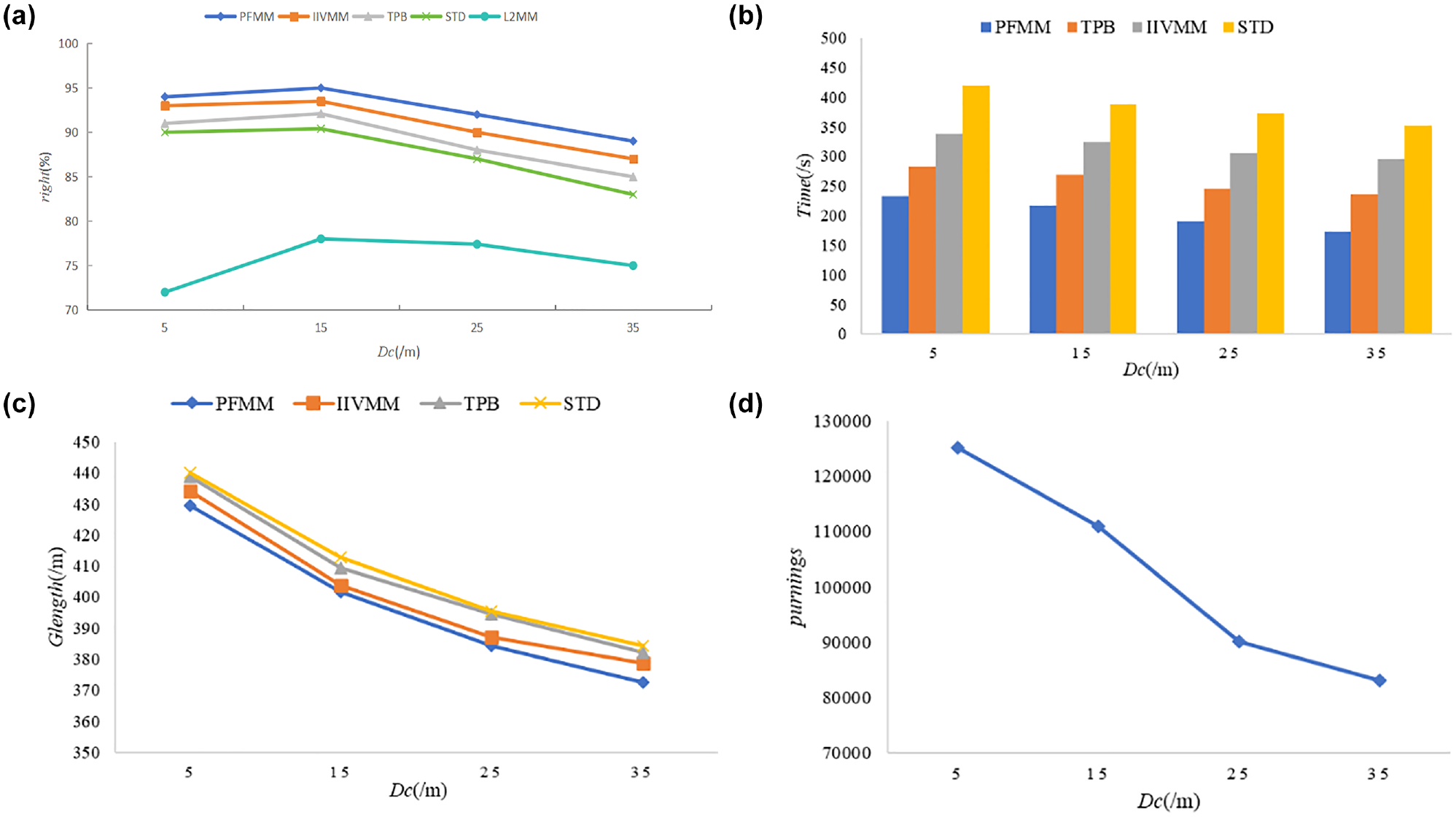
The impact of distance threshold (Dc) value on algorithms: (a) The impact of distance threshold (Dc) value on algorithms rights; (b) The impact of distance threshold (Dc) value on algorithms Time; (c) The impact of distance threshold (Dc) value on Glength; and (d) The impact of distance threshold (Dc) value on pruning.
Impact of Number of Candidate Points (k)
This section compares the performance of the PFMM, IIVMM, STD, and L2MM algorithms for different values of the number of candidate points (
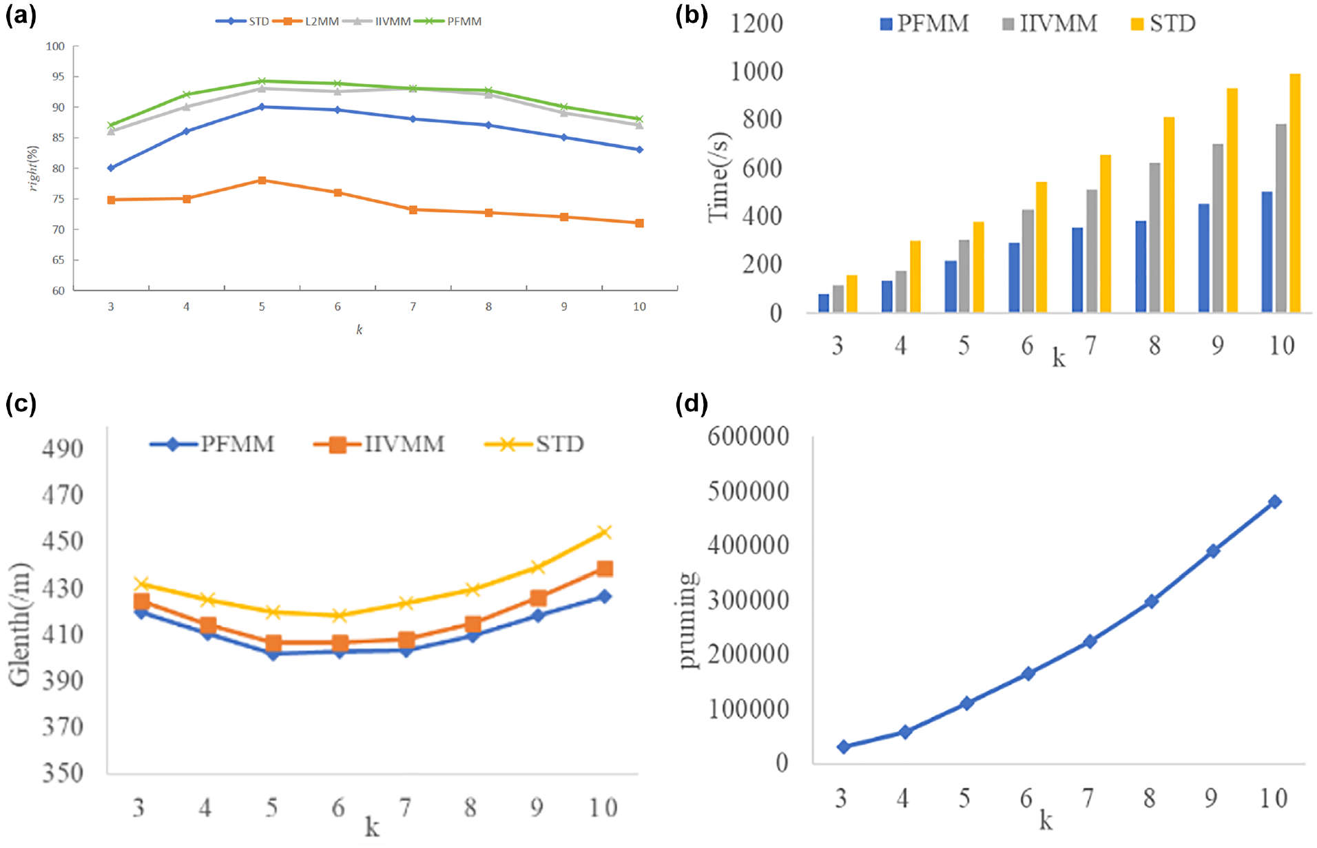
The impact of the number of candidate points (k) value on algorithms: (a) The impact of candidate points (k)value on algorithms rights; (b) The impact of candidate points (k) value on algorithms Time; (c) The impact of candidate points (k) value on Glength; and (d) The impact of candidate points (k) value on pruning.
Impact of Candidate Search Radius (r)
This section describes the effect of changing the candidate point
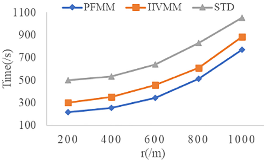
The impact of search radius (r) value on algorithms.
Algorithm Performance at Different Sampling Frequencies
In this section, the trajectory dataset is resampled and the algorithm performance of the PFMM, IIVMM, TPB, STD, and L2MM algorithms is compared for trajectories with different sampling frequencies.
Figure 14a shows the difference between the PFMM algorithm in this paper and the comparison algorithm when comparing the Right values for trajectories with different sampling frequencies. The PFMM algorithm has a 2.2% higher Right than other existing algorithms, the difference between the Right of the PFMM algorithm and the IIVMM is smaller, and the PFMM performs better at low sampling rates and can improve the algorithm performance in complex road conditions because of the inclusion of pre-selected point analysis. The performance of the algorithm in complex road conditions is improved by the inclusion of pre-selected point analysis. The PFMM algorithm reduces the cost of shortest route computation by pruning with a bounded value rule. On average, the running time cost of the PFMM algorithm is reduced by 29.6% and the matching efficiency is significantly improved. Figure 14c shows the variation of the algorithm’s matching route length at different sampling frequencies. This is because, when the sampling frequency is too high, the algorithm directly queries the shortest route between two points and considers fewer trajectory points; on average, the matching route length of the PFMM algorithm is reduced by 4.6% compared with other algorithms. Figure 14d shows the change in the number of prunings for the PFMM algorithm, with fewer trajectory points and fewer prunings as the sampling frequency increases.
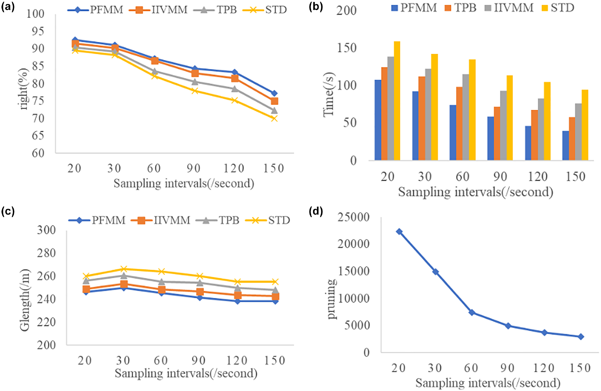
The impact of sampling intervals value on algorithms: (a) The impact of sampling intervals value on algorithms rights; (b) The impact of sampling intervals value on algorithms Time; (c) The impact of sampling intervals value on Glength and (d) The impact of sampling intervals value on pruning.
Conclusion
This paper investigates the map-matching problem based on GPS trajectories. Compared with existing work, this article provides a faster and more accurate mapping processing method, and proposes a secondary computation candidate point extraction strategy and a fast matching strategy based on limited value pruning to solve the bottleneck and accuracy problems of existing map-matching algorithms in routing computation. The algorithm makes use of road intermediate point information and considers more factors in the candidate point extraction stage to improve the matching accuracy; meanwhile, two pruning strategies and the IDijkstra routefinding algorithm are proposed to reduce unnecessary routing computations and thus improve the matching efficiency. In addition, the initial trajectory is processed by outlier filtering and dwell point detection methods, which reduce the number of trajectory input GPS points and lower the computational cost, providing a more efficient and accurate solution for map-matching applications. This helps to improve the efficiency and accuracy of some specific problems in the Geographic Information System (GIS) field, such as navigation processing and traffic management. The map-matching algorithm proposed in this paper is suitable for offline scenarios, to which a real-time matching prediction model can be added in subsequent work to make it applicable to real-time scenarios and reduce latency. Through this article, we provide readers with a novel approach to solving the mapmath problem. In future work, we will extend this method to big data environments, using parallel and distributed methods to solve the mapping problem in large-scale data, to cope with the growing traffic data. The code of our model are available on our GitHub repository (https://github.com/bugerror404/mapmatch.git)
Footnotes
Author Contributions
The authors confirm contribution to the paper as follows: study conception and design: Bai Mei, Niu Yujing; data collection: Li Chunye, Wang Xite; analysis and interpretation of results: Ma Qian, Li Guanyu; draft manuscript preparation: Bai Mei, Niu Yujing. All authors reviewed the results and approved the final version of the manuscript.
Declaration of Conflicting Interests
The author(s) declared no potential conflicts of interest with respect to the research, authorship, and/or publication of this article.
Funding
The author(s) disclosed receipt of the following financial support for the research, authorship, and/or publication of this article: This study was supported by the National Natural Science Foundation of China (Grant numbers 62002039, 61702072, 61602076, and 61976032).