
Abstract
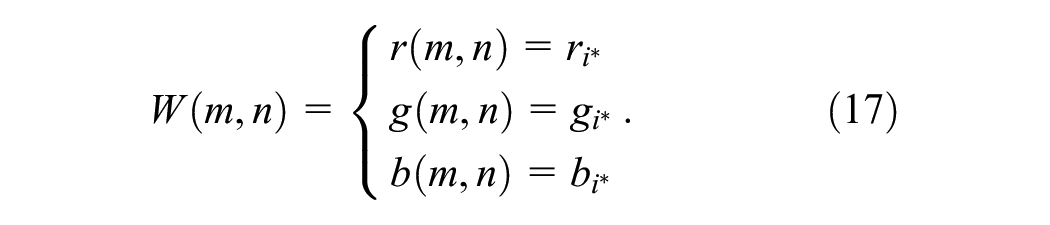
Blind zones in light detection and ranging (LiDAR) sensors arise from their limited physical field of view and obstructions caused by static infrastructure or moving objects. Although originally intended for vehicle-based applications, LiDAR sensors are now increasingly deployed in roadside infrastructure for traffic monitoring and connected and automated vehicle safety and mobility applications. However, there is a dearth of robust tools for analyzing their detection range, resolution, and other characteristics in such settings. This study introduces a three-dimensional (3D) blind zone simulation model for analyzing the detection characteristics of roadside LiDAR sensor deployment. The model replicates the impact of static infrastructure conditions and dynamic blind zones during live traffic. Initially, a real-world digital surface model (DSM) captures 3D data of road surfaces and obstructing infrastructure objects. Optical geometry models then assess blind zone severity across various roadway areas. Subsequent 3D vehicle shape and dynamic simulations evaluate blind zone distributions under typical traffic conditions. The model’s effectiveness is validated using field 3D point cloud data and vehicle detection data collected from a roadside LiDAR site on Route 18 in New Brunswick, NJ. Evaluation results demonstrate the model’s capability in analyzing complex static and dynamic blind zone distributions, offering insights for optimizing LiDAR sensor location, height, tilting angle, and manufacturer configuration parameters to minimize sensing blind zones. For code availability, see https://github.com/rutgerstslab/LiDAR-Coverage-Analysis.
Keywords
Light detection and ranging (LiDAR) sensors utilize laser beams to determine the distance and three-dimensional (3D) location and shape of objects. LiDAR sensors can perform vehicle tracking ( 1 – 4 ), accurate speed estimation ( 1 ), vehicle classification ( 2 , 5 ), and pedestrian detection ( 2 , 6 – 8 ). LiDAR has made significant advancements in functionalities, range, resolution, form factors, and affordability, driven by the growing demand from the self-driving industry. Although LiDAR sensors have been extensively used in on-board advanced driver assistance system and automated driving system platforms, roadside LiDAR technology has emerged as a promising sensor support solution for enhancing connected and automated vehicle (CAV) applications. Several studies have explored the integration of roadside LiDAR into transportation applications, including aiding traffic operations ( 1 ), enhancing transportation safety ( 6 , 8 ), and supporting CAV applications with high-resolution trajectory data ( 6 – 8 ). Overall, roadside LiDAR sensors demonstrate promising potential to enhance real-time situational awareness and decision-making.
High-resolution roadside sensing from LiDAR, computer vision, and other sensors provides excellent opportunities to overcome the biggest weakness of prevailing connected vehicle (CV) system deployment. The current low penetration rate of CV on-board units (OBUs) in general traffic and regulatory actions on shrinking the designated dedicated short-range communication bandwidth by the Federal Communications Commission ( 9 ) means that traditional CAV system designs relying on in-vehicle OBUs may not be feasible in the near term. The high-resolution sensors can track the movements of vehicles, pedestrians, motorcycles, bicycles, and other objects and create basic safety messages and personal safety messages on their behalf without the need for on-board units—that is, full participation of all road users.
Roadside LiDAR sensing operates differently from on-board LiDAR sensing for self-driving. Roadside LiDAR sensors are installed at a fixed roadside location, making their coverage stay at the same location with a fixed infrastructure background. Such coverage ( 10 ) differs from on-board LiDAR sensing, which experiences more dynamic backgrounds because of vehicle movement. This distinction simplifies the reduction and removal of roadside LiDAR background data ( 11 ). Additionally, the fixed installation eliminates the need for extensive real-time simultaneous localization and mapping operations. Compared with on-board LiDAR, roadside LiDAR has a wide variety of vehicles and full 24 × 7 infrastructure coverage as a trade-off for limited geographical coverage. Recent research in transportation technology has significantly improved traffic safety and operational efficiency with roadside LiDAR. Zhao et al. ( 2 ) emphasize the need for real-time cooperative systems with infrastructure-mounted LiDAR sensors to enhance situational awareness for all road users, particularly in scenarios prone to occlusion, where their proposed solution involves deploying multiple LiDAR sensors to extend detection range and mitigate obstructions. Kloeker et al. ( 12 ) introduce a framework for the quality evaluation of smart roadside infrastructure sensors, offering insights into sensor setup configurations for automated driving applications and smart cities. Du et al. ( 13 ) present a life-cycle monitoring framework that employs high-precision positioning and perception data from CAVs to assess the accuracy of roadside sensor data throughout their operational life cycle within cooperative vehicle infrastructure systems.
Despite the promising potential of roadside LiDARs in enabling CAV applications, the design and planning tools or methods for roadside LiDAR installation still need to be improved. Like other line-of-sight (LOS)-based sensors, LiDAR cannot penetrate objects and is therefore affected by the blind zones caused by infrastructure objects and vehicle occlusions. It blocks part of the 3D space whenever something is detected, creating a blind zone that the sensor cannot “see.” A recent study by the research team developed a preliminary two-dimensional (2D) blind zone simulation model for roadside LiDAR design and planning ( 14 ). The simulation model takes into account the 2D geometry of the roadway and uses basic optical geometric models to simulate the blind zone distribution for a roadside installation on a leveled, flat, and clear infrastructure background but with dynamic vehicle trajectory inputs such as Next Generation SIMulation (NGSIM) datasets. The model can assess the impact of basic roadside LiDAR configuration parameters and provide insights into how LiDAR blind zones are distributed within live traffic. However, the model does not consider the 3D terrain and complex infrastructure conditions in the real world and assumes that all vehicles are traveling on a straight road through a rectangular grid system without considering vehicle orientation or attitude because of roadways’ horizontal and vertical curves.
In this paper, we proposed several key features to create a comprehensive LiDAR blind zone simulation model suitable for real-world LiDAR deployment design, planning, and blind zone analysis. First, a digital surface model (DSM) is proposed to reconstruct real-world 3D roadway and roadside infrastructure. Second, the simulated vehicles can now have additional degrees of freedom, including orientation and attitude. Third, flexible 3D shapes of vehicles can now be considered, and their full interaction with 3D road surfaces can be modeled. Last but not least, a sensing overlapping analysis module is introduced to allow multi-sensor configuration. We also designed new computational-efficient occlusion determination methods to enable the above new features. With these new capabilities, the simulated blind zone model is validated with field LiDAR data at the grid level and is used for roadside site planning and design in the DataCity Smart Mobility Testing Ground project. The dynamic DSM-based 3D reconstruction is efficient in both computation and transmission and is ready for large-scale real-time digital twin visualizations. The LOS computing method fully utilizes the efficiency of DSM and only require 2D LOS determination plus one height comparison for z-axis, instead of 3D frustum. Compared with the authors’ prior work, the proposed LiDAR blind zone analysis model mainly has the following improvements. (1) Real-world 3D road surface is sampled in the form of DSM for sensor location evaluation, including multi-sensor deployment. (2) Preprocessing is designed to smooth the DSM for road user placement and movement simulation. (3) Real-world trajectories are mapped and embedded into the 3D road surface with actual position and 3D orientation to reflect the impact of complex behaviors such as lane changing, making turns, and climbing slopes. (4) The redesigned the parallel-computable per grid occlusion determination has stable performance against large-scale trajectories. (5) Different LiDAR sensors are compared and valuable insights are generated for both sensor manufacturing and deployment.
Literature Review
The existing literature has explored the impact of different vehicle-mounted on-board LiDAR sensor configurations on 3D object detection and tracking in self-driving applications. The impact of different configuration parameters and design elements have been considered, including physical design perspectives ( 15 ), information-theoretic surrogate metrics ( 15 ), and Bayesian theory-based evaluations ( 16 ) to mixed-integer linear programming ( 17 ) and bio-inspired cost functions ( 18 ). Hu et al. ( 15 ) introduced an information-theoretic surrogate metric, called Surrogate Maximum Information Gain (S-MIG), to quantitatively and efficiently evaluate different on-board LiDAR configurations and their impact on detection performance, including center (Argo AI), line (Ford), pyramid (Cruise and Pony AI), and trapezoid (Toyota). Their experiment demonstrates a correlation between S-MIG and detection performance. However, S-MIG is more efficient, as it does not require performing the actual detection. Ma et al. ( 16 ) proposed a perception entropy-based metric to model the perception potential of candidate on-board sensor configurations based on Bayesian possibility theory. Dybedal and Hovland ( 17 ) proposed a method and accelerated it with a graphic processing unit (GPU) ( 19 ) to handle cases where several sensors must cover certain sub-volumes (redundancy). The objective function includes maximizing the number of cubes covered by the sensors and minimizing the cost of the sensors needed to cover the entire area. Liu et al. ( 18 ) used a bio-inspired measure called the volume-to-surface-area ratio as a cost function representing the size of non-detectable subspaces of a given LiDAR configuration to address the optimal LiDAR configuration problem for autonomous vehicles. Kim et al. present multi-sensor placement methods for multiple LiDAR sensors on an autonomous vehicle ( 20 ) and roadside infrastructure in urban environments ( 21 ). For autonomous vehicle LiDAR configuration ( 20 ), the objective is to find optimal LiDAR positions that reduce the dead zone and improve the point cloud resolution. The problem is formulated as an optimization problem using the LiDAR occupancy grid and solved by a genetic algorithm. Experimental results using commercial LiDAR devices demonstrate the effectiveness of the proposed method in improving LiDAR placement. For roadside infrastructure ( 21 ), they analyze the dead zone caused by buildings near the intersections with a voxel-based LiDAR occupancy space and LiDAR occupancy voxel grid. The evaluation is done with different simulation scenarios involving both pedestrians and vehicles. The authors also mention future extensions of the method to incorporate sensor fusion with multiple LiDARs, radars, and cameras into the autonomous vehicle system.
Point cloud simulation has recently been introduced to evaluate and optimize different roadside LiDAR sensor placement and configuration scenarios. Ge et al. ( 14 ) proposed a 3D simulation model for roadside LiDAR sensor blind zones. The model takes different location, height, and tilting scenarios of the LiDAR sensors and field vehicle trajectory and size data, such as NGSIM data, and can run LOS simulation for all LiDAR beams to evaluate the spatial and temporal distribution of blind zone areas where LiDAR cannot penetrate in live traffic. However, the model cannot take complex road geometries with curves, 3D terrain changes, and complex roadside infrastructure. The LOS assessment can be quite computationally extensive for large-scale simulation. Cai et al. ( 22 ) proposed an optimization framework for infrastructure LiDAR sensor placement using LiDAR point cloud simulation within the CARLA (CAR Learn to Act) simulator environment. Their approach incorporated various simulation effects, such as motion distortion and ghosting object effect. Although the simulation did not account for different weather conditions, it included trajectories from OPV2V ( 23 ). The optimization is based on a performance metric, the laser density on the infrastructure through predefined LiDAR occupancy boards ( 24 ). The existing simulation-based roadside LiDAR sensor performance evaluation models are limited by their reliance on preexisting models or their inability to accommodate complex road geometries and infrastructure. Gouda et al. ( 25 – 27 ) proposed the use of octree-based point cloud simulation for infrastructure LOS analysis and compared it with traditional voxel-based simulations ( 28 ). The octree-based method surpasses traditional voxel-raycast approaches in accuracy and practicality for evaluating traffic sign visibility in autonomous vehicle scenarios. Octree-based methods are commonly employed in general 3D data representations, particularly for sparse point cloud data. The advantage of using octrees in LOS simulation lies in their ability to determine LOS more efficiently without requiring detailed examination of every smallest voxel. However, these methods do not fully leverage the specific characteristics of road traffic, leaving room for further efficiency improvements when embedded with dynamic trajectories.
Building on the authors’ earlier work ( 14 ), this paper presents a computationally efficient 3D simulation of LiDAR sensor blind zones that can formulate complex roadway infrastructure, 3D terrain conditions, and detailed 3D dynamic traffic; proposes a more efficient parallel LOS computing method; and adds support for multi-sensor situations. Furthermore, the model is independent of traffic simulation or simulator models, so field vehicle trajectory data can be used to perform sensor placement and configuration optimization with real-world data. Meanwhile, the model still preserves the ability to interact with traffic simulation and simulator models through vehicle trajectory data.
Methodology
Notations and Definitions
Basic Concept
The proposed method is designed for complex field deployment scenarios in roadside instrumentation. The DSM is used to formulate the 3D terrain and roadway infrastructure ( 30 ). Correspondingly, to simulate vehicles traveling over roads with horizontal and vertical curves, the vehicle attitude (pitch) is added as an additional dimension in vehicle movement simulation. Combined with the vehicle shape and trajectory data, the proposed method will be able to model the 3D dynamics of vehicles in the complex infrastructure conditions in the field. However, the increased complexity caused by the high-resolution DSM formulation poses computational challenges to the proposed LiDAR LOS simulation. We propose new model formulations and parallel computing algorithms for efficient processing of the DSM and LiDAR data for occlusion detection.
DSM
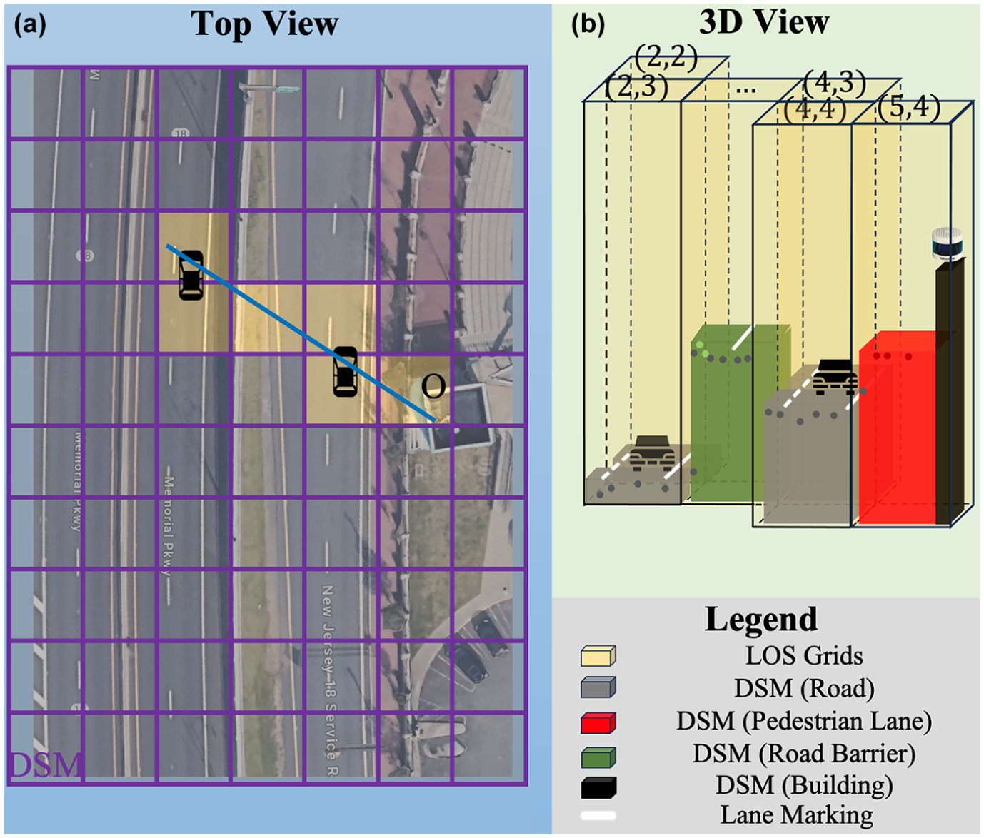
As Figure 1 shows, a DSM is a 3D grid-based surface representation of a real-world terrain and infrastructure condition generated from LiDAR or photogrammetry point cloud. In the field, a road infrastructure’s point cloud data can be collected using vehicle-based LiDAR scanning or drone-based aerial scanning. LiDAR scanning obtains the precise 3D locations of infrastructure points scanned by the laser beams of LiDAR sensors. Drone-based aerial scanning generates a point cloud by matching and triangulating features between overlapping aerial images or video frames.
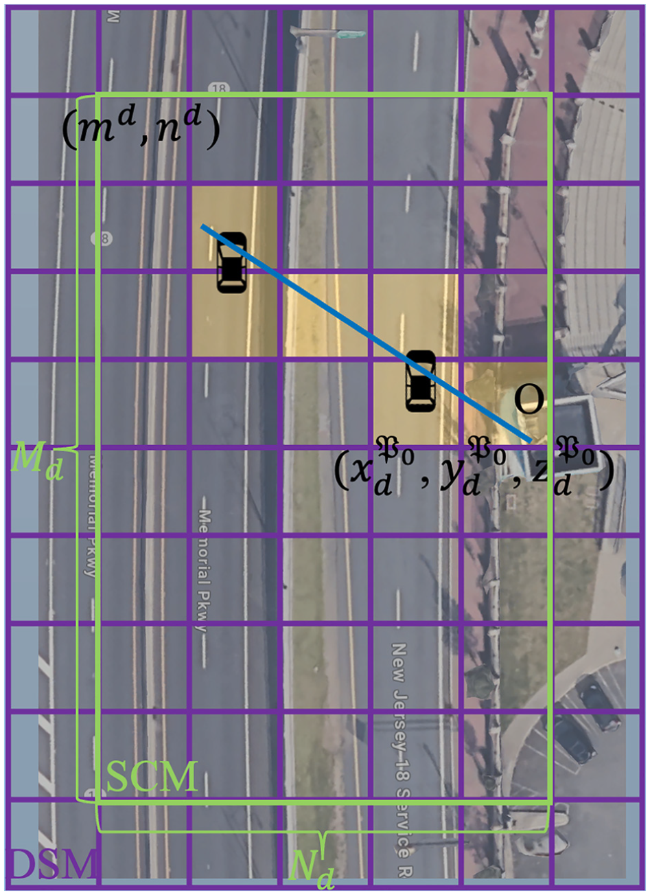
Top view of digital surface model (DSM) and sensor coverage model (SCM) grid scheme (Vehicle Icons: 29).
From the availability perspective, the digital elevation model (DEM) is widely available across the country, and the proposed DSM-based method is compatible with DEMs. DEMs can be separated into digital terrain models and DSMs based on the elevation they are collected from. From an efficiency perspective, the proposed method utilized the DSM structure that accurately describes the road surface with dynamic traffic information. Compared with voxel-based methods, the proposed DSM-based method is more efficient because it stores the height information of a 2D map instead of all the 3D information. The occlusion determination is also simplified to 2D plus one height comparison instead of considering the entire frustum. Compared with octree-based methods, generating and updating the DSM with dynamic traffic is less complex, and the DSM-based information can be summarized in quadtree. As the trade-off, the DSM-based method has trouble handling complicated 3D information, which is acceptable for road traffic simulation. We define DSM as
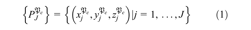
The DSM is constructed in three steps. First, we project the point cloud
Multi-Source Point Cloud and Map Coordinate System Matching and Unification
The input data to construct the proposed DSM model includes three different data sources: (1) the satellite imagery from the World Map of ArcGIS in NAD83 (North American Datum of 1983) world coordinates, (2) colored photogrammetry point cloud collected from a drone with centimeter-level accuracy with projected coordinates in meters, and (3) high-resolution millimeter-level uncolored LiDAR point cloud collected from vehicle-based LiDAR scanning. The first data source uses world coordinates in longitudes and latitudes, whereas the other two use their own projected coordinate system, with their origin set at different locations within the study area. Furthermore, the validation and evaluation study for the proposed model also requires the output to be matched with the relative coordinate systems used by LiDAR sensor data centered at the locations of the LiDAR sensors. Since such multi-source scenarios are quite common when working with field geospatial data, a generic method is proposed below to align different coordinate systems with reference points across all models.
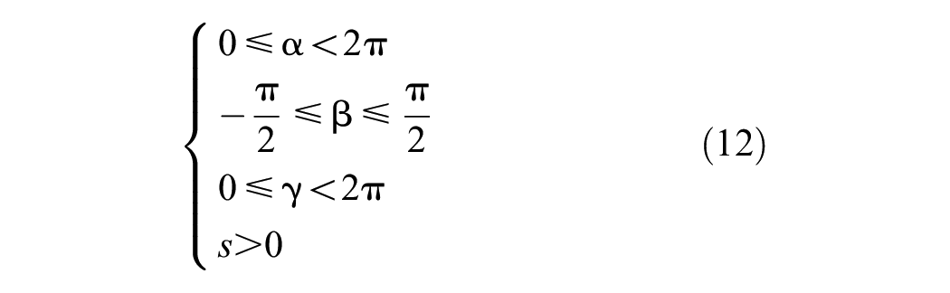
The proposed alignment method is an optimization formulation with respect to a series of coordinate system transformation parameters, including rotation angle yaw
where
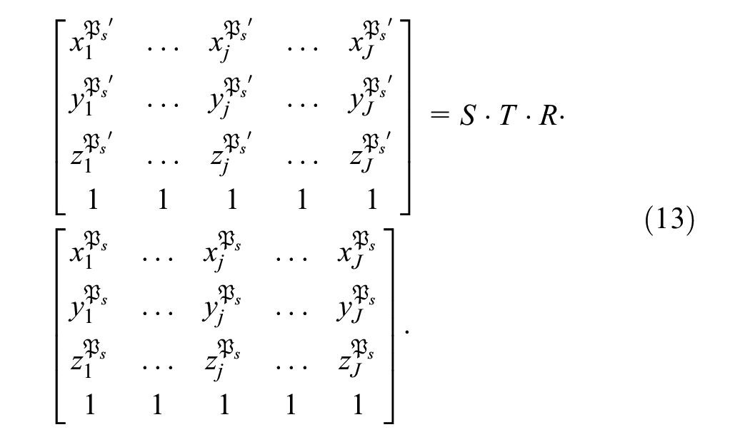
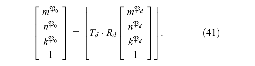
The problem becomes finding the correct 3D transformation matrix to transform the coordinates of the reference points from a coordinate system other than the target coordinate system (
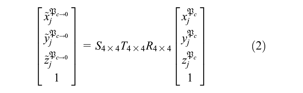
where
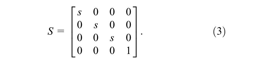
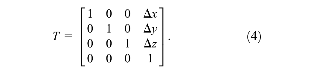
The translation matrix accounts for the combined movement along the three axes as follows:
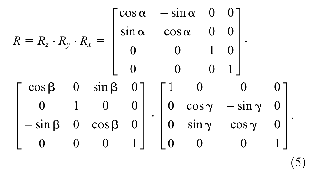
Finally, the rotation matrix accounts for the combined rotations around all three axes, including yaw (along the z-axis), pitch (along the y-axis), and roll (along the x-axis).
With the above matrices defined, the generic optimization problem can be formulated as follows:

where

Then, with the calculated matrix
Objective function simplification. Since the purpose is to group 3D points into 2D grids, we can further simplify the objective function to focus on correcting the longitude and latitude. Since the trajectory placement and blind zone analysis are based on relative elevation, this approach does not affect accuracy for a single DSM analysis. However, when expanding to a larger area, additional effort is required to align different DSMs to the same elevation because of the absence of real-world elevation data:

3D rotation simplification.
The Nelder–Mead simplex method (
31
) can be used to minimize the variance of

The initial value for

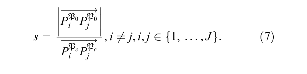
Translation offsets calculation. With the rotation factors determined through Equations 7 and 8,

The final expanded optimization formulation is as follows:
minimize
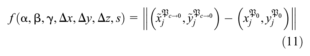
subject to
where
Digital Surface Calculation
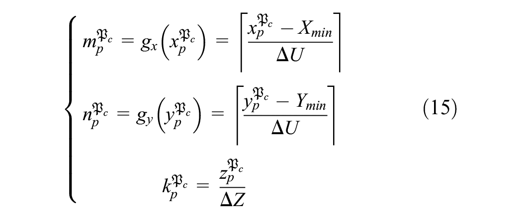
With the matched and unified 3D model and point clouds, we can flatten the point clouds into 2D representations along the z-axis with respect to a DSM gridding system at the targeted resolution. As Figure 2 shows, for each grid, we need to determine the RGB color and height of the top points in DSM. The flattening process starts with defining the 2D

where
Real-world DSM sampling. (a) Grid scheme of experiment site. (b) 3D laser status.
Then, we group all the 3D points in the point cloud by the corresponding grids with parallel computing and then calculate the largest z-value to be set as the height for a specific grid. For each point
where

Then let
Point Cloud Z-Value Smoothing
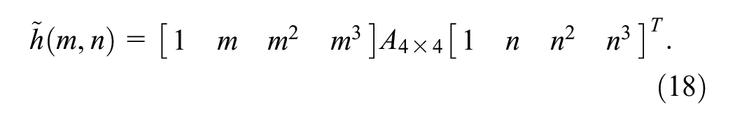
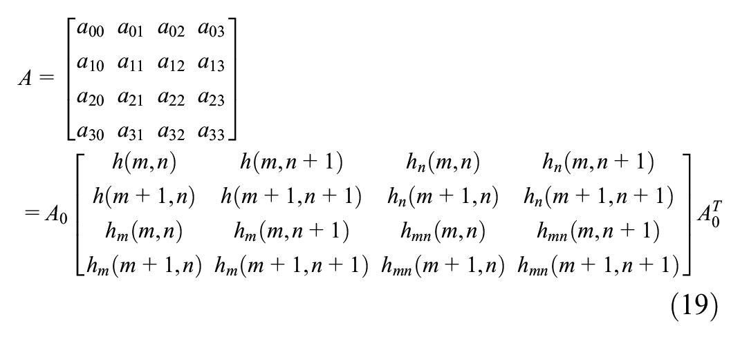
Real-world point cloud datasets may also contain holes and spikes because of the limitation of 3D reconstruction technologies or the appearance of vehicles and other moving objects shown during scanning. Such issues can worsen with drone-based videogrammetry technologies. Significant holes on the ground can appear because of the lack of matched features for the 3D triangulation of pixels in the image. To solve this issue, we apply the bicubic interpolation ( 32 ) to fill the empty holes on the road surface and surrounding infrastructure (e.g., medians and barriers):
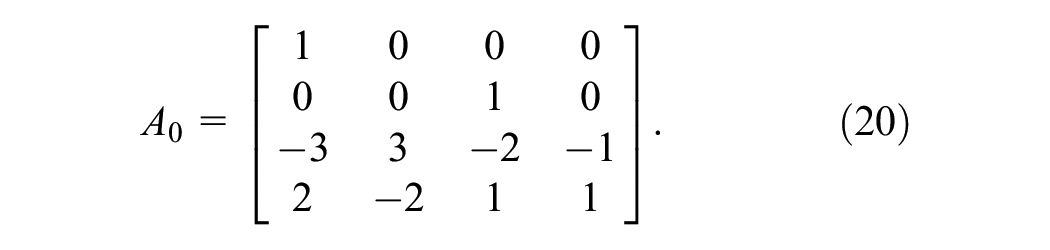
The coefficient matrix
where
The partial derivatives

In the proposed simulation model, this is implemented with the Python SciPy package.
For spike removal, the goal is to smooth out abnormal heights that exist in

where
where
Road Sign and Overhead Power Line Removal
During the generation of DSM, the grids with road signs and overhead power lines will use the top of the signs/wires for the grid heights, which cannot correctly reflect the occlusion. To mitigate those incorrect blind zones, we can filter out the narrow signs and wires from the DSM with morphological operation, opening ( 34 ), which is usually used to first erode an image and then dilate the eroded image to remove small objects and thin lines from an image while preserving the shape and size of larger objects in the image. We can directly apply it to the DSM and update the grid heights like modifying pixel colors of an image.
Dynamic Vehicle Placement
We can further expand the DSM with the time dimension
where
To simplify the calculations, here we assume that the slope change is not significant so that we can simulate the vehicle pitch altitude by aggregating the vehicle heights over the DSM.
Because of the lack of 3D vehicle shape, we generate random heights
We can create a DSM-like array
First, we can reuse Equation 15 to calculate the vehicle center in the grid coordinate system
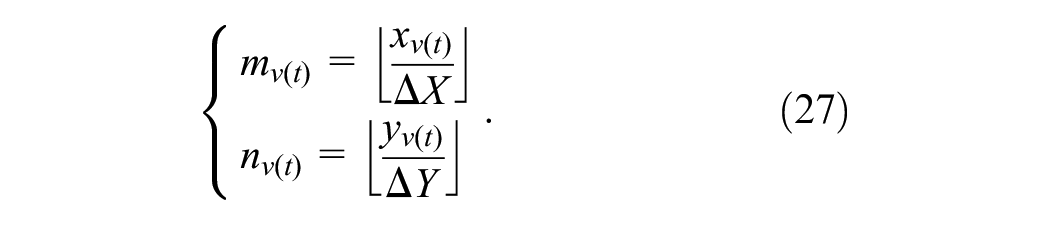
With width
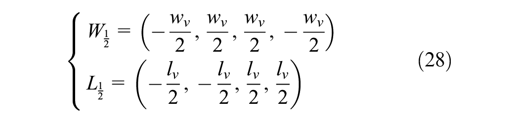

where
Then, for any grid
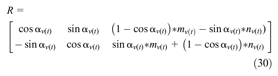
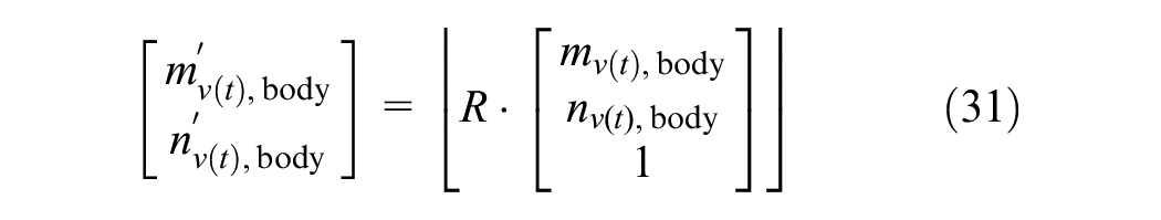
where
After getting the vehicle grids, we can place the heights (e.g.,

where
After updating the height of every vehicle in time

where
LiDAR SCM
In practice, the roadside LiDAR instrumentation can involve multiple sensors to create coverage overlaps to minimize the impact of occlusions and ensure continuous coverage along a corridor. Similar to the definition in Ge et al. ( 14 ), the “blind zone” of roadside LiDAR sensors refers to (1) the built-in occlusions caused by preconfigured vertical field of view (FOV) designed for mounting on top of vehicles and (2) occluded areas caused by the infrastructure or the moving vehicles blocking the LOSs. To analyze the blind zone in the proposed model, we introduce the LiDAR SCM, whose spatial area is a subset of DSM, to record the coverage details of the LiDAR at different grids within DSM.
We denote the LiDAR SCM of sensor
Single-Sensor Single-Beam Grid Height Calculation
The simulation of the coverage of a LiDAR sensor starts with the computation of the height of each beam

where

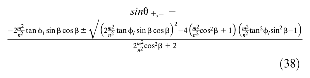
If sensor
where

The two roots are reflected in the formula of
Integration of Multi-Sensor SCMs to DSM
It should be noted that the above two steps are most computationally efficient when the calculation of LiDAR laser beam heights in SCM is executed in the original coordinate system of the raw LiDAR point cloud. Then, the grids of SCMs containing the calculated results are converted into the DSM gridding system without the need to convert the massive raw or simulated LiDAR point cloud data into the DSM coordinate system. Given the SCMs of multiple sensors in their original coordinate systems,
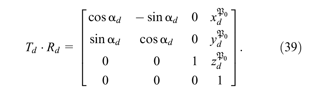
Then, the coordinate transformation equation from
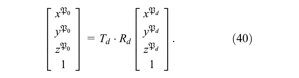
Given
SCM Laser Beam Segment-Based Blind Zone Status Determination
The proposed blind zone status determination model can be applied to static infrastructure and roadway infrastructure with dynamically moving objects such as vehicles, pedestrians, motorcycles, bicycles, and so forth. It should be noted that the blind zone status can vary in 3D space above a grid
As shown in Figure 3, to analyze each LiDAR
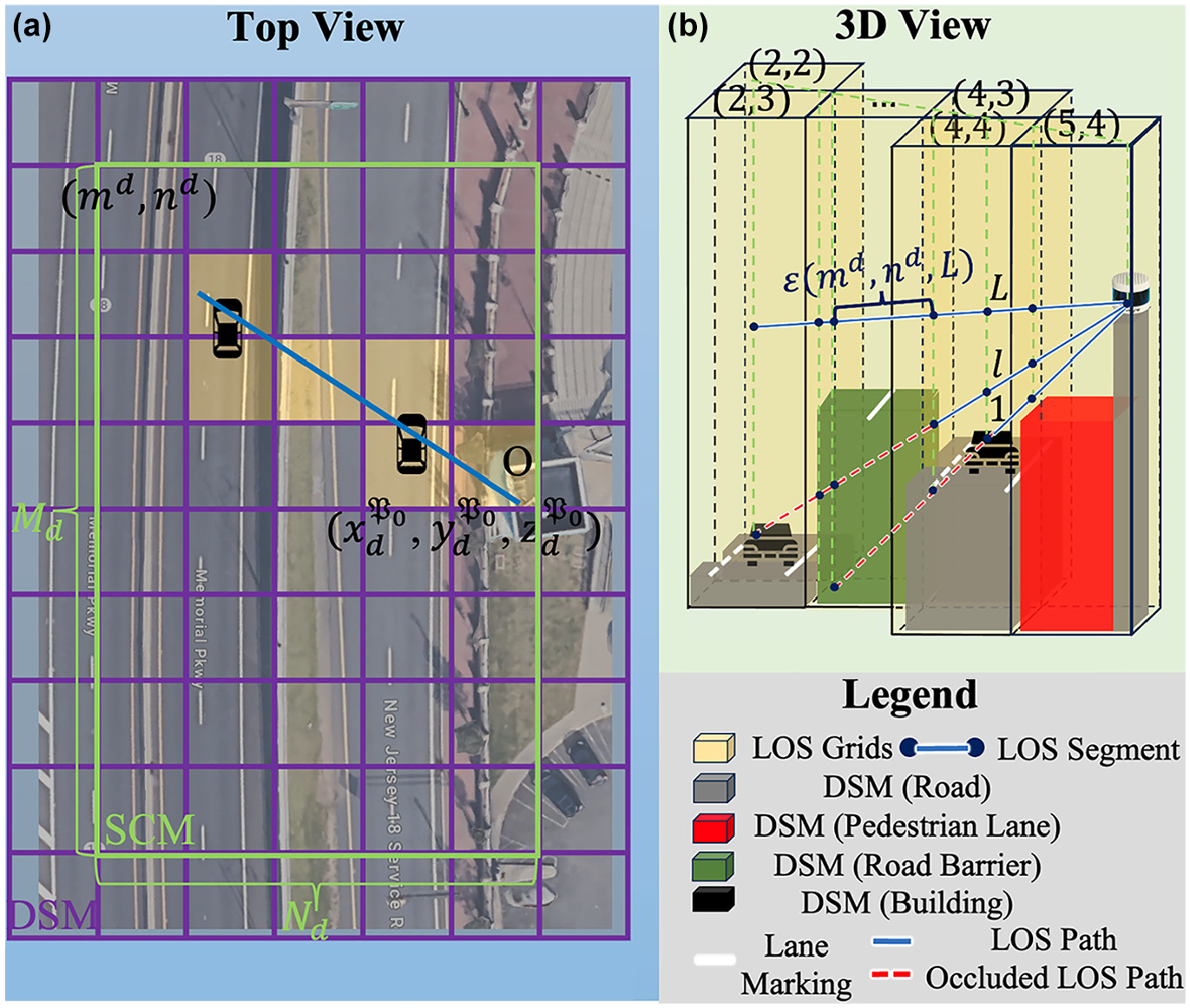
Real-world laser beam sampling and DSM comparison. (a) Grid scheme of experiment site. (b) 3D laser status.
Within the SCM,
Occupancy. Any elevation of a grid can be occupied by a moving object (O) (e.g., a vehicle, a bicycle, a motorcycle, a pedestrian, etc.), by an infrastructure object (I), and be vacant for road users to traverse (V).
Detectability. Any grid elevation is detectable by a laser beam when the laser beam can penetrate the entire path from the LiDAR sensor origin to the grid without being occluded (D); otherwise, the grid is not detectable (N).
We denote each segment
OD: An occupied (O) detectable (D) LOS segment.
ON: An occupied (O) but undetectable (N) LOS segment.
VD: A vacant (V) detectable (D) LOS segment.
VN: A vacant (V) but undetectable (N) LOS segment.
ID: A LOS segment occupied by infrastructure objects (I) that is detectable (D).
IN: A LOS segment occupied by infrastructure objects (I) that is undetectable (N).
With the above analysis, the lowest LOS segment among all the laser beams that can reach the current grid determines the blind zone height in the current grid. VN and ON LOS segments are the targeted occlusion and detectability status to define blind zones considered in this paper. It should be noted that V/O is determined by ground truth rather than the LiDAR detection results. VN and ON status can be derived from grid occupancy statuses in ground truth infrastructure and moving object conditions from a simulation-based design and planning study or alternative sensors in field evaluation studies (e.g., drone-based aerial sensors).
Figure 4 shows the detailed process of the proposed quantized laser status determination methods. The quantization means that even though the LOS segments may have different distances in different grids because of the 3D traversing angles of laser beams, we consider only their grid-by-grid detectability and occlusion status and thus irrelevant to the segment lengths.
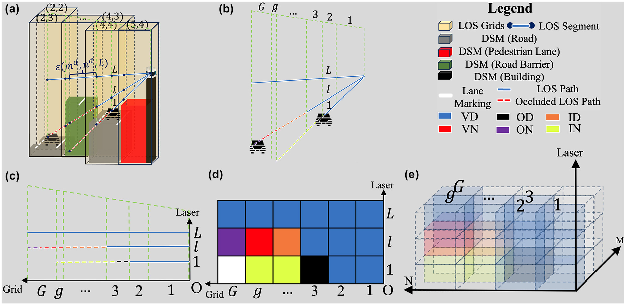
Quantized laser status. (a) 3D laser status. (b) Extracted laser status. (c) Laser status by laser ID. (d) Quantized two-dimensional (2D) laser status. (e) Quantized 3D laser status (Vehicle Icons: 39).
Figure 4a shows sample laser beam paths from Figure 3b. The laser path’s coloring shows the different occlusion statuses of the LOS segments. Figure 4, b–d, shows how the blind zone status matrix
We only need to record the laser ID and its occlusion and detection status in each grid, since we can always retrieve the corresponding height information from
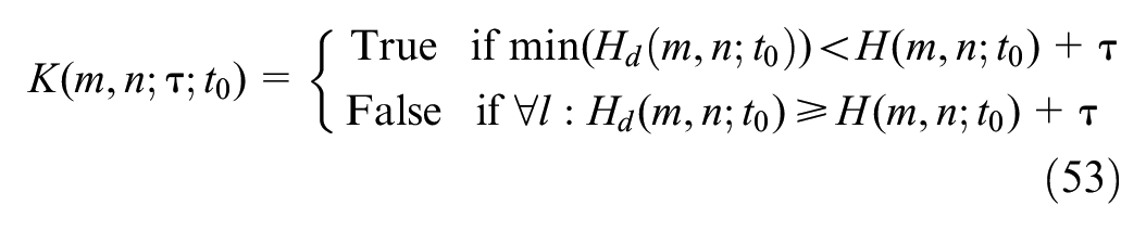
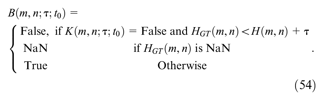
The objective of blind zone determination is to segment the 3D space into six categories: ID, VD, OD, IN, VN, and ON. To achieve this objective, we only need to determine the occupancy and detectability status by comparing the SCM height matrix
The occupancy status in ground truth or reference data for each LOS segment
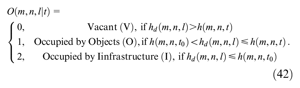
Meanwhile, the detectability status for each LOS segment
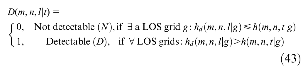
where
With the occupancy and detectability status, we can infer the category based on Table 1 and fill up
Dynamic SCM Zone Type Determination
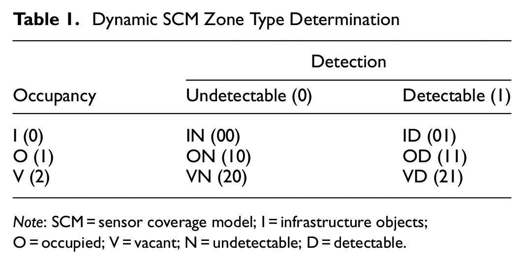
Note: SCM = sensor coverage model; I = infrastructure objects; O = occupied; V = vacant; N = undetectable; D = detectable.
Grid Blind Zone Status Determination
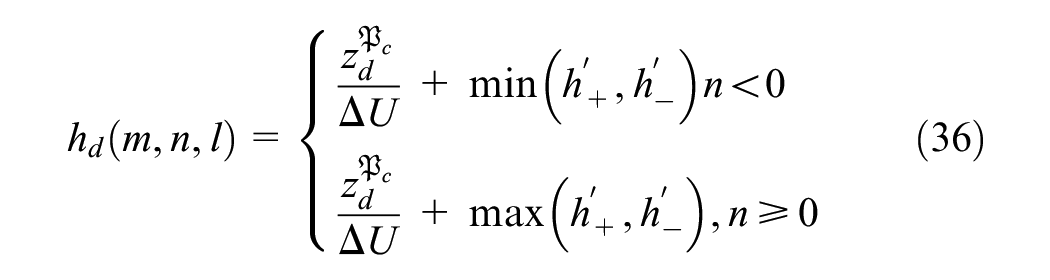
The final blind zone status in a grid is determined as follows:

where
Combined with the trajectory, the proposed model can determine the grid status based on real-world detection demands. For roadway traffic-sensing applications, it is not necessary for the LiDAR devices to see the ground. Instead, as long as the road user is higher than the lowest laser, the LiDAR can sense the user. Furthermore, for most scenarios, the road users will have their lanes to travel, and there can be a lenient requirement for the grids where the traffic will not travel through. In other words, we can get the statistically lowest road user height
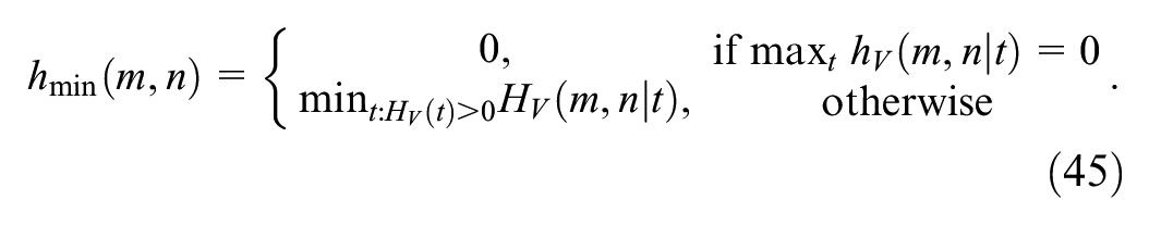
Then, we can use
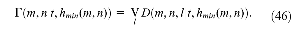
The result of Equation 46 ensures the lowest road user can always be sensed by at least one laser and is fundamental for sensor(s) placement.
Experiment Design
Data Source
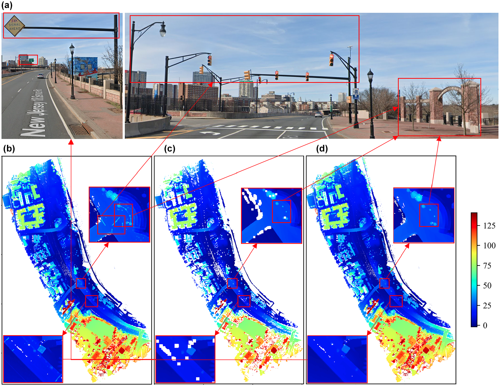
In the experiment design, the proposed dynamic blind zone detection model is implemented on a DSM generated from a real-world 3D model with vehicle trajectories retrieved from roadside LiDAR data. The proposed SCM is deployed over grids of 0.3 m × 0.3 m, consistent with the DSM. The LiDAR sensor Velodyne Alpha Prime is installed on the roof of a roadside infrastructure near Boyd Park, New Brunswick, NJ, as depicted in Figure 5, a–c. This location is part of the New Jersey Department of Transportation DataCity Smart Mobility Testing Ground project and is equipped with one 128-beam LiDAR and two 2K cameras.
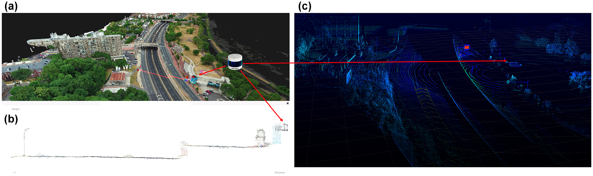
Data source. (a) Three-dimensional (3D) model. (b) Surface elevation. (c) Light detection and ranging (LiDAR) point cloud data.
As Figure 5a shows, the 3D point cloud data used in the DSM are from a 3D model generated by videogrammetry in the projected coordinate system of NAD83 (EPSG [European Petroleum Survey Group]: 3615) ( 37 ) from a drone flight executed on June 11, 2023.
The dynamic LiDAR data were collected on August 17, 2023, between 5:50 and 6:00 p.m. The trajectories retrieved by Ouster’s Bluecity Solution ( 38 ) comprise 1,843 unique road users within 5,901 frames (99 frames without detections). The data fields used as the simulation inputs include location information (local_x, local_y) and shape information (length, width, and type). Vehicle types were used to infer the vehicle heights based on typical design vehicle values ( 39 ).
The real-world LiDAR background data used as ground truth for validation were collected from the same LiDAR sensor. The background determination is based on the LiDAR data processing results when no vehicles are detected. The specific time is 1:37 a.m. on July 26, 2023.
As depicted in Figure 5, b and c , the surface elevation shows Route 18 splitting into two levels, and the occlusion caused by the higher-level infrastructure and traffic poses a significant challenge in sensing lower-level traffic. The proposed paper generates the DSM from the 3D model and validates it with LiDAR data. The static blind zone is validated and evaluated based on the 3D laser distribution of field LiDAR data and simulated LiDAR data. Meanwhile, the dynamic blind zone is evaluated based on actual trajectories collected from the same location.
DSM Validation Metrics
Height Difference between DSM and LiDAR
As the base of the simulation, it is essential to evaluate the accuracy of the DSM before performing any evaluation on the simulation model. If the DSM coordinate systems perfectly match that of the LiDAR sensor, all the LiDAR data should stay right on the DSM. For each grid
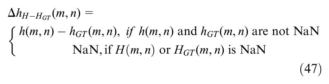
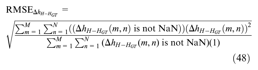
where
However, in practice, we found that there were some outliers caused by distant high buildings, which significantly increased the


where
Grid-Based Percentage Error of DSM
After getting the height offset and the tilting (pitch) offset of the LiDAR sensor, we can further look into the detailed grid matches to approximate the 2D location
where
SCM Validation
With the empty frame of LiDAR point cloud data without any vehicle, we can compare it with the simulation model by sampling the LiDAR point cloud data into the same resolution as the simulation model using Equation 15 and getting the lowest height of the point cloud in each grid.
Grid-Based SCM Verification
The SCM provides the whole 3D spatial distribution
where
Then, we can compare the lowest LiDAR point cloud data
The lower the
To be noted,
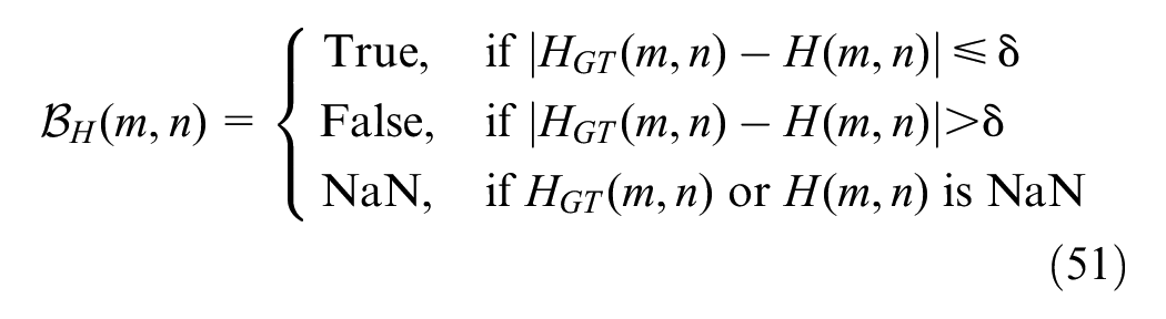
Static Blind Zone Evaluation
The background causes a static blind zone, and the static blind zone pattern is relatively permanent once the roadside sensor is installed.
Blind Zone Height
The blind zone height (14)

where
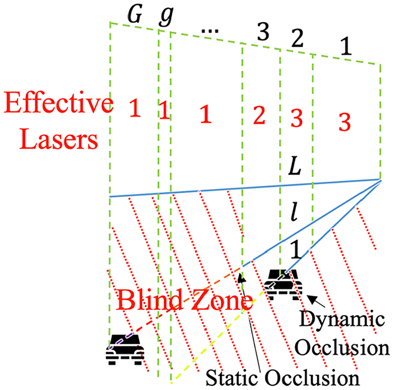
Blind zone height and effective laser count (Vehicle Icons: 39).
Laser Count
Given HOI
where
Laser count is meaningful for evaluating the detection and reconstruction potential of the sensor data. Having more laser beams within the HOI
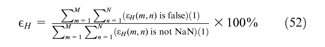
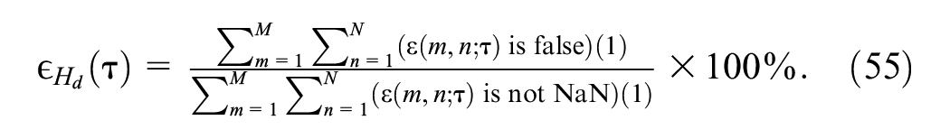
Percentage of Unoccluded Lasers
In addition to the laser count, we can emphasize the impact of occlusion by calculating the percentage of unoccluded lasers

where
Dynamic Blind Zone Evaluation
Unlike the limitation of the static blind zone evaluation, in dynamic blind zone evaluation, we can get ground truth points in the blind zone covered lanes. As Figure 5 shows, the right-most lane on the lower level is in the blind zone. The importation of the vehicles brings the hope of getting some points on the vehicles when they pass the blind zone.
Temporal Mean and Percentile Blind Zone Height
We can use the temporal mean and percentile of blind zone height ( 14 ) over time to evaluate the severity of the blind zone affected by the dynamic traffic with regard to detecting the traffic. Take mean blind zone height, for example:

where
Temporal Mean Laser Count
We can use the temporal mean of laser count

where
Aggregated Time in Blind Zone and Maximum Consecutive Time in Blind Zone
Aggregated time in the blind zone
Analysis of Results
DSM
Coordinate System Calibration
As Figure 7 shows, with three pairs of reference points, the 3D photogrammetry model is matched with the real-world coordinate system. Figure 7a shows the selected three distant points. Figure 7b shows the flattened model placed over Google Maps. By doing this, the calibrated 3D model can be verified to have the correct north and up directions. With the three pairs of matched coordinates from Google Maps, we can calculate the geo-information for the 3D model. Figure 7c shows the GeoTIFF file generated from the 3D model that can be directly imported into ArcGIS/ArcMap. GeoTIFF is based on the TIFF format and is used as an interchange format for georeferenced raster imagery. From Figure 7c, we can see that NJ-18 and its ramps are properly aligned and the lanes are well matched at the boundaries.
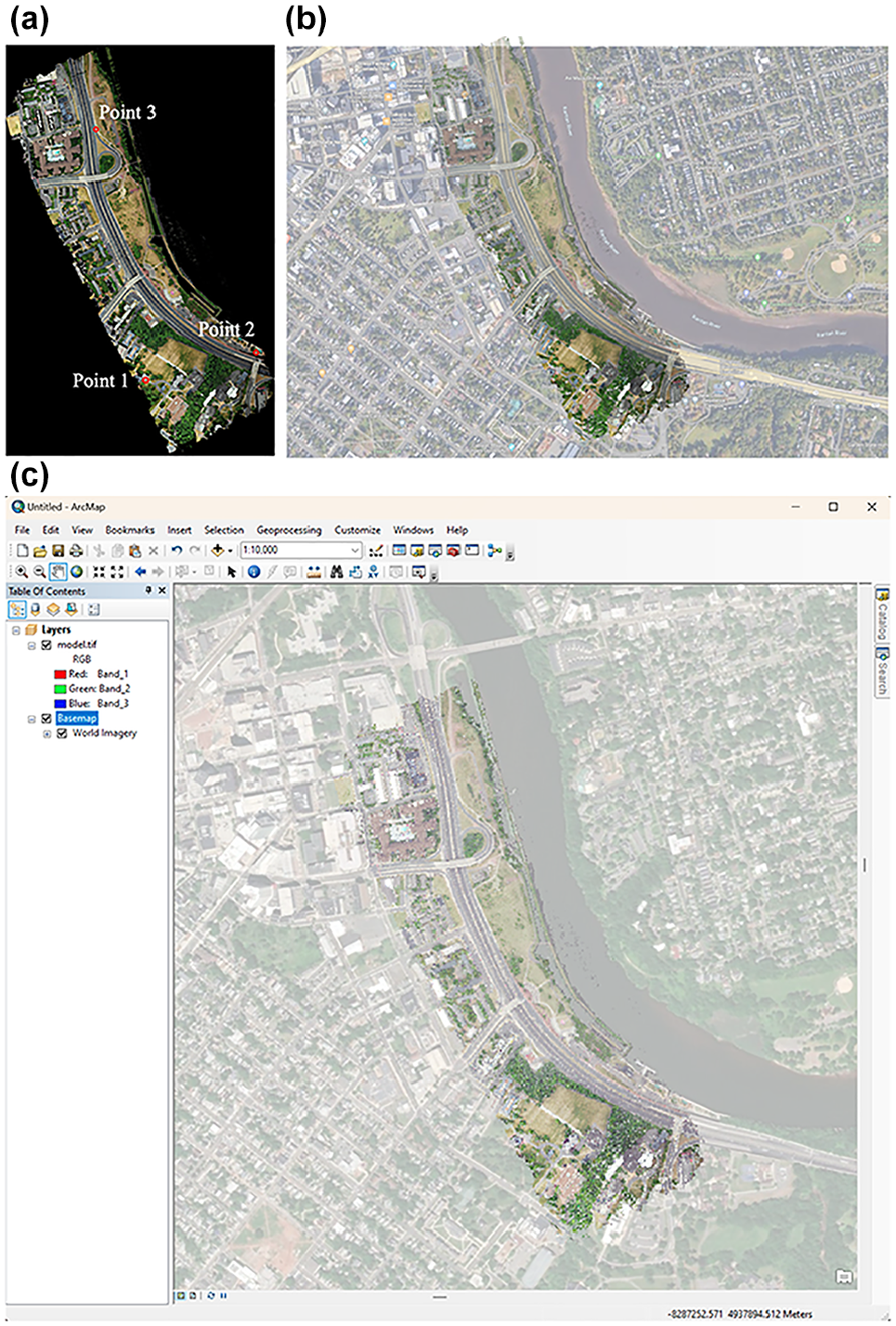
Coordinate system calibration result. (a) Manually picked reference points. (b) Flattened three-dimensional (3D) model matched with Google Maps. (c) GeoTIFF with coordinates visualized in ArcMap.
DSM Generation
Figure 8, a–d, shows the 3D views of the DSM filtered by different Gaussian kernels. The 3D model was generated from high-angle drone video and had a lot of noise. The noise affects the DSM quality, as Figure 8a shows. By applying the Gaussian filter, we can see the results with different
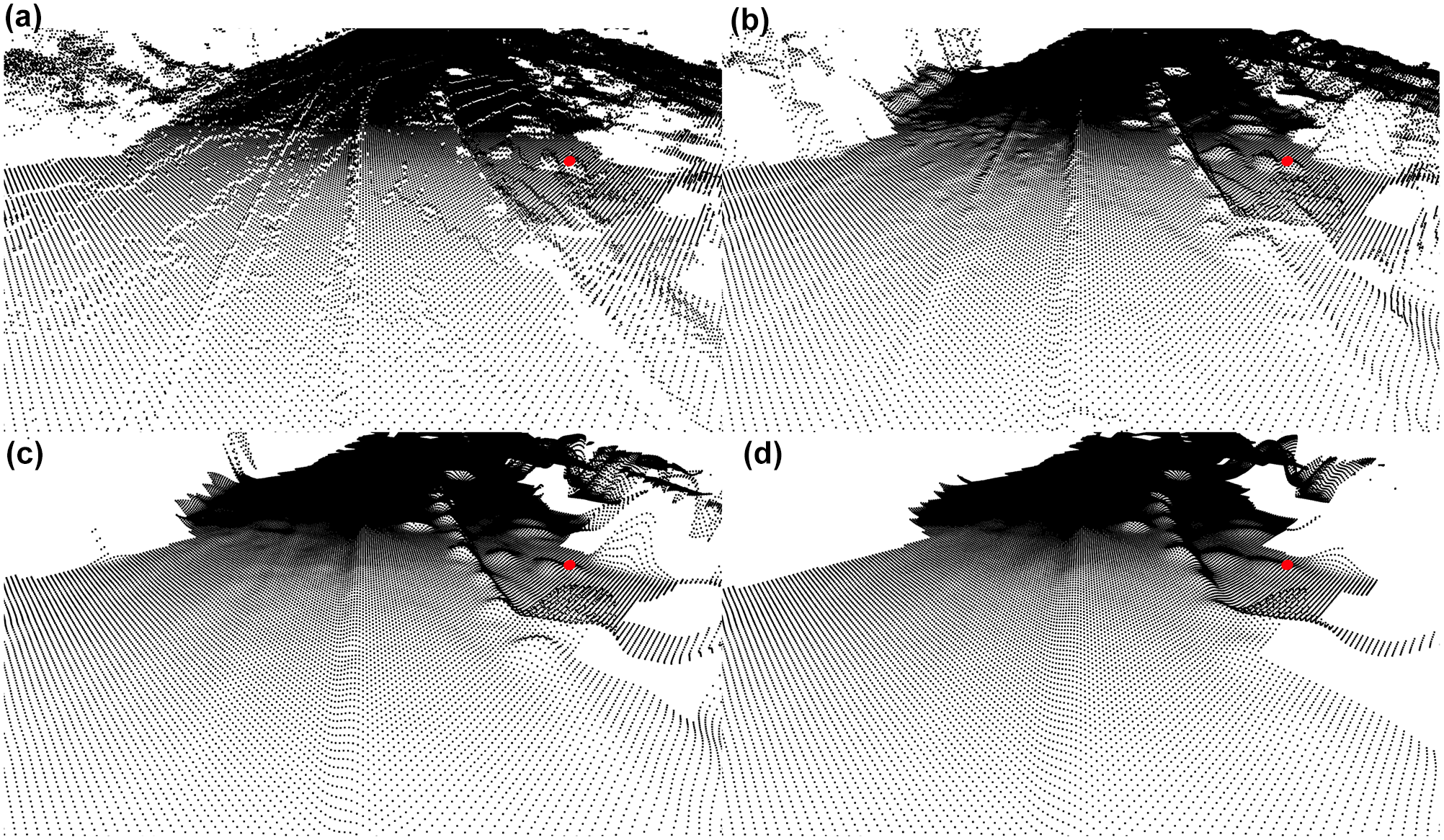
Gaussian smoothed digital surface model (DSM) with different
Figure 9 shows the road sign and overhead power line removal. Figure 9b shows the original DSM that contains the road signs. It is correct, but it will not cause blind zones that affect the real-world traffic sensing. Figure 9, b and c , shows the DSM processed by morphological operations that no longer reflects road signs or overhead power lines while deliberately retaining the thick vertical pillars. By removing those higher objects from the DSM, a more realistic blind zone can be simulated.
Road sign and overhead power line removal with image opening. (a) Street view. (b) Digital surface model (DSM). (c) DSM after opening. (d) Combined DSM.
DSM Validation
Figure 10a shows the top view of the 3D model for DSM, focusing on the sight of interest (SOI) of the simulation. The white blocks mean that there are no available heights in the grids. Figure 10b shows the top view of the LiDAR data over the SOI. Figure 10d shows the height difference between DSM and LiDAR
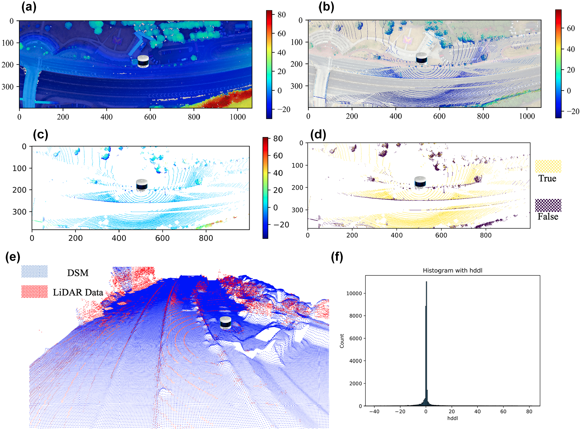
Digital surface model (DSM) calibration. (a) DSM over the sight of interest (SOI). (b) Light detection and ranging (LiDAR) data over the SOI. (c)
SCM
SCM Validation
Figure 11a shows the ground pattern of the simulation model with
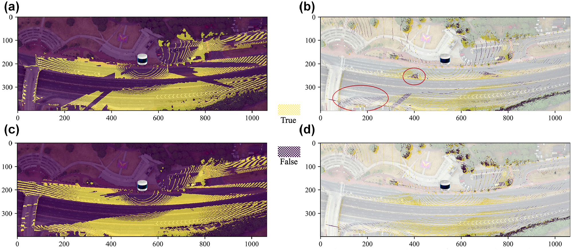
Sensor coverage model validation. (a) Ground pattern with
Similarly, because we have slightly changed the position of the virtual LiDAR to avoid it being completely occluded by the real LiDAR and other roadside instruments, the blind zones caused by nearby poles and trees are at different angles in the bottom left. However, it does show a problem, as has been red-marked, that a large sign installed on a thin pole will raise the DSM to the top of the sign, which is not correct in the real world. Similar problems will also happen to the gantries, which are not shown in the figures.
Figure 11, c and d , shows the simulated ground pattern and the validation after removing the road signs with morphological operations. The red-marked blind zones in Figure 11b are correctly mitigated. However, compared with Figure 11b, the actual LiDAR ground pattern, some thin poles were also removed from the DSM, and some actual blind zones were incorrectly mitigated. Therefore, the morphological operations should be used cautiously when necessary. For example, removing the overhead wires in the city street is necessary. Otherwise, the wires in the DSM will occlude the lasers like high walls.
Static Blind Zone Evaluation
With the advantage of simulations, static blind zones can be calculated by placing no traffic in the background. With regard to their contribution to traffic safety and management, both static and dynamic blind zones can affect sensor coverage and hinder the roadside system’s ability to predict near-miss events. However, static blind zones can be easily calculated and subsequently avoided or mitigated during the design phase. In contrast, dynamic blind zones require actual or simulated trajectories that accurately reflect traffic patterns, such as traffic flow, large vehicle ratios, and vehicle distances. To analyze dynamic blind zones during the design phase, accurate microscopic traffic simulations are essential.
Figure 12 shows the laser count
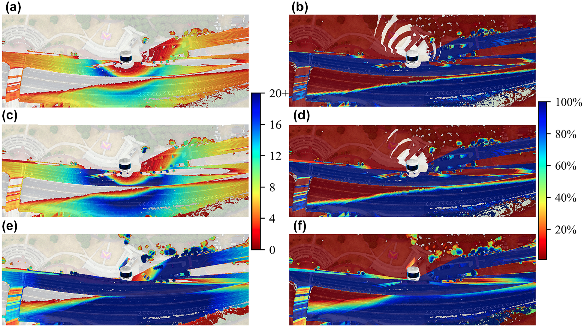
Laser count and percentage of unoccluded lasers within
Dynamic Blind Zone Simulation
Figure 13 shows dynamic LiDAR simulation results for four frames at 2-s intervals and a special case frame. The left side of Figure 13 illustrates the ground pattern of the LiDAR laser beams affected by the traffic, whereas the right side shows the corresponding blind zone height, ranging from 0 to 14+ ft above the ground.
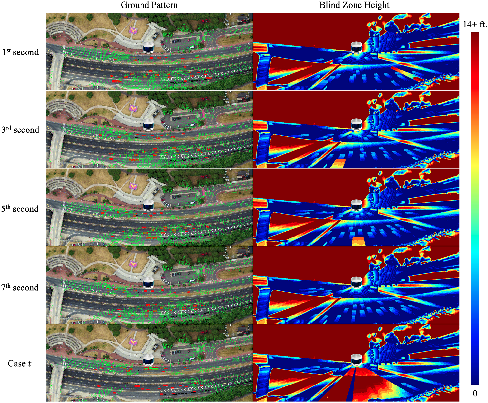
Dynamic light detection and ranging (LiDAR) simulation.
For the upper-level traffic, because of both the shorter distance and the higher vehicle positions, the dynamic blind zone caused by large vehicles on the upper level may affect both the upper-level sensing and the lower-level sensing, as the special case at time
Dynamic Blind Zone Evaluation
We can further look into actual traffic to analyze the dynamic blind zone. Figure 14 shows the blind zone heights aggregated by frames over
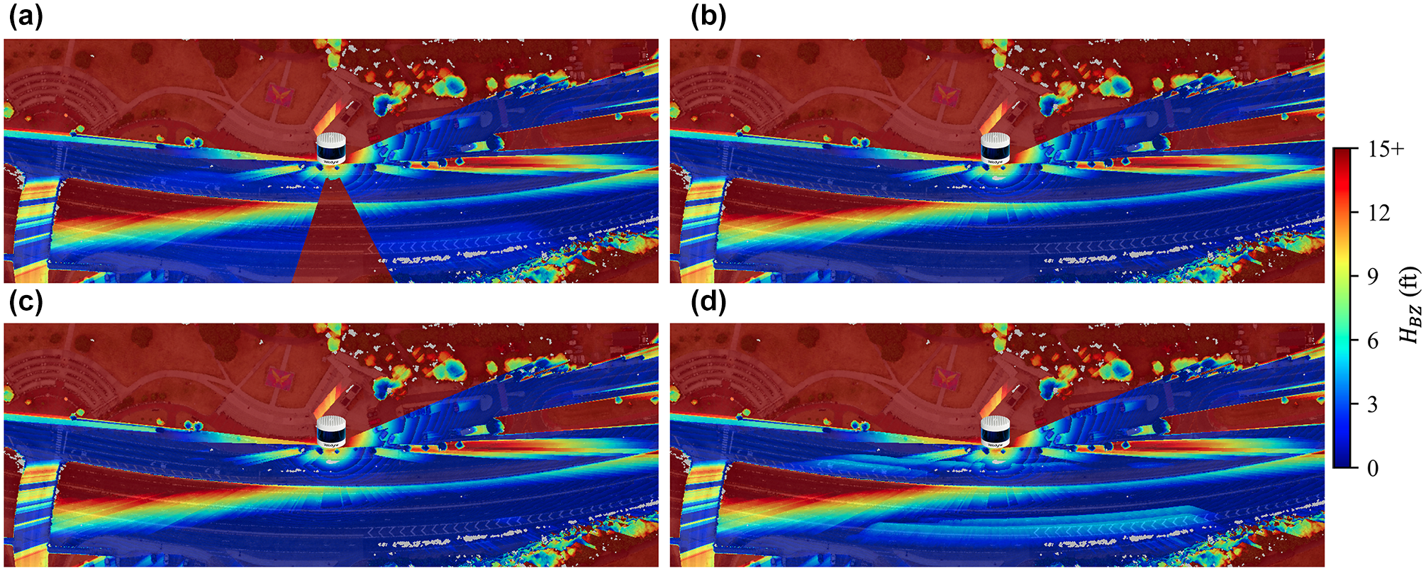
Mean and 15th, 85th, and 100th percentiles of temporal aggregated blind zone height (above ground). (a)
Although the blind zone height in Figure 14d is not optimistic, we can still count on the tracking algorithm to predict if there is any road user on the occluded grid. Figure 15 shows the grid-based blind zone duration and the maximum consecutive time in the blind zone at HOI levels of 4, 6, and 14 ft, representing the heights of sedans/coupes, SUVs/pickups, and trucks. Ignoring the elephant in the room, since the static blind zone will last “permanently,” we can explore how the traffic affects the dynamic blind zone. Figure 15, a, c, and
e
, shows the percentage of total time in the blind zone. As Figure 15a shows, even for
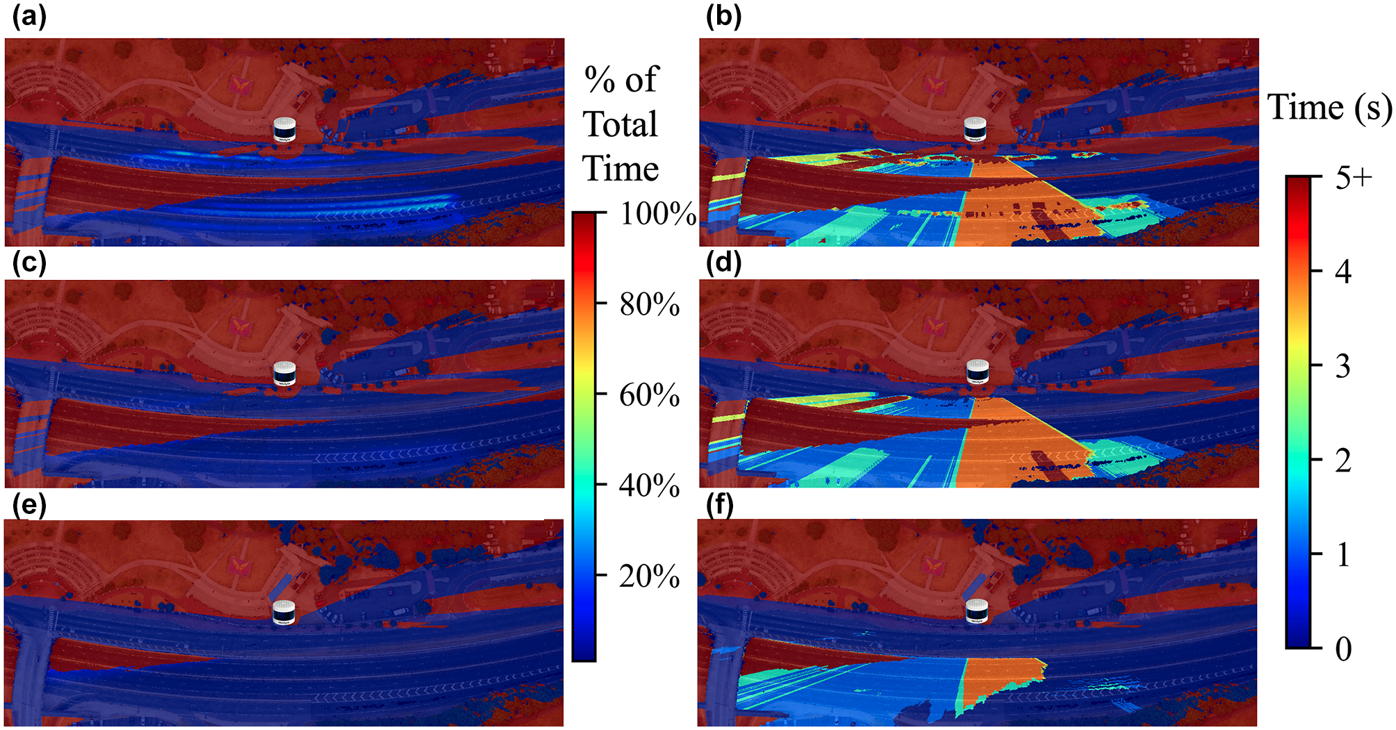
Time in the blind zone and maximum consecutive time in the blind zone. (a) Time in the blind zone—4 ft above ground. (b) Maximum consecutive time in the blind zone—4 ft. (c) Time in the blind zone—6 ft above ground. (d) Maximum consecutive time in the blind zone—6 ft. (e) Time in the blind zone—14 ft above ground. (f) Maximum consecutive time in the blind zone—14 ft.
The major issues with this LiDAR setup are the infrastructure-caused static blind zone on the lower level and the large vehicle-caused blind zone. Limited by regulations, power availability, and geometry, the positions and heights of the sensors are restricted. However, we can explore potential solutions, such as trailer sites with solar power.
Multi-Sensor Blind Zone Evaluation
We can place more sensors and evaluate the coverage to enhance the sensing capability and gather more information from the site.
By adding one LiDAR looking from the lower level, the blind zone caused by the infrastructure can be significantly reduced. Figure 16 shows the LiDAR ground pattern generated using Equation 53. Figure 16, a and b , shows the ground pattern using only one LiDAR. In Figure 16a, the infrastructure causes significant static blind zones because of elevation differences. In Figure 16b, to make the LiDAR able to cover the upper level, it has to be installed much higher, making the traffic below the LiDAR invisible. If we combine both LiDAR devices, as Figure 16c shows, the coverage is significantly improved, and dense LiDAR lasers cover the whole road surface.
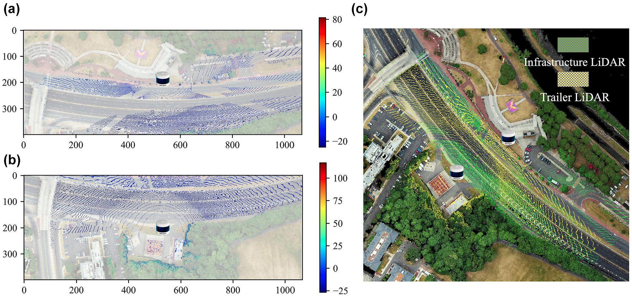
Multi light detection and ranging (LiDAR) ground pattern with one trailer-based location. (a) LiDAR ground pattern—infrastructure location. (b) LiDAR ground pattern—trailer location. (c) Fused LiDAR ground pattern.
Figure 17 shows the lowest blind zone height map for two sensors. The improvement achieved by using two sensors is significant compared with using any single LiDAR sensor in this complex scenario. The static blind zone caused by terrain and infrastructure is well covered. The mesh-like pattern in Figure 17c results from resampling during mapping the two results onto the same DSM and should be disregarded; the actual blind zone does not exhibit this pattern. However, this introduces new challenges in sensor placement optimization, as multi-sensor placement problems can become exponentially more complex.
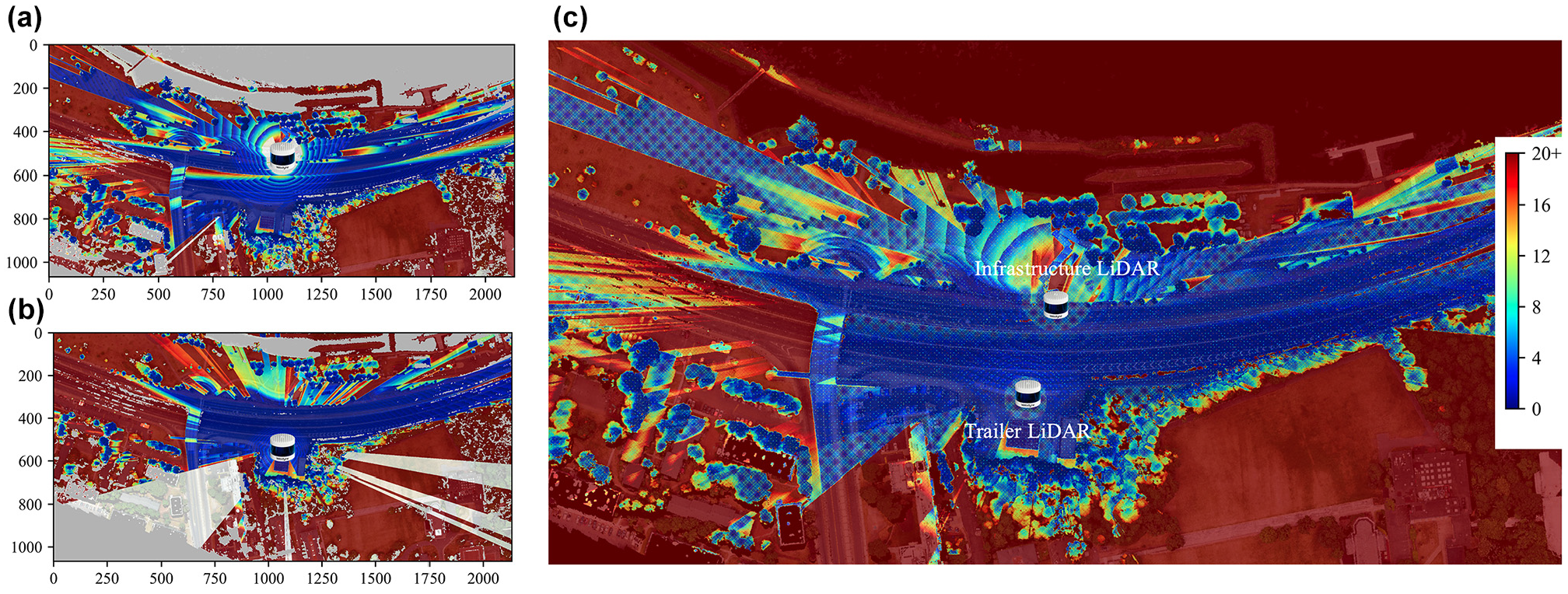
Blind zone height map of multi-sensor setup. (a) Light detection and ranging (LiDAR) blind zone height map—infrastructure location. (b) LiDAR blind zone height map—trailer location. (c) Fused LiDAR blind zone height pap.
Dynamic Blind Zone Height Map of Different LiDAR Devices
As Figure 18 shows, model VLP-16 has 16 laser beams distributed between −15° and 15°, HDL-32E has 32 beams distributed between −30° and 10°, and Alpha Prime has 128 beams distributed between −25° and 15°. With all of them installed at 23 ft with 10° tilting toward the roadway, it is obvious that HDL-32E benefits from its −30° vertical FOV range and has a smaller blind spot beneath the LiDAR than the other two models. However, with significant more lasers, Alpha Prime has better robustness against occlusion-caused blind zones thanks to the smoother blind zone boundaries. For roadside LiDAR deployment, it is important for the manufacturers to not only increase the laser beams but also expand the vertical FOV further downwards.
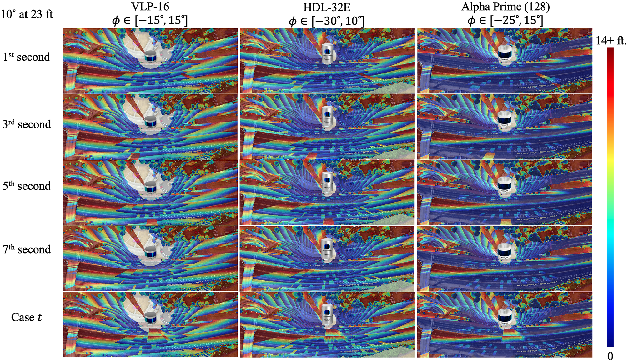
Dynamic blind zone height map of different light detection and ranging (LiDAR) devices (VLP-16, HDL-32E, and Alpha Prime).
Statistical Blind Zone Analysis of Different LiDAR Devices
Figure 19 shows some interesting patterns for comparison of different LiDAR devices. Unlike Figure 18, Alpha Prime leads the performance because of its 128 lasers, especially for the laser count within 4 ft above ground. It also relieves some areas from the blind zone duration. From the average blind zone height and laser count within 4 ft above ground, neither the 16-beam LiDAR VLP-16 nor the 32-beam LiDAR HDL-32E can satisfy the demand for road traffic reconstruction or even just tracking under the multi-level roadway condition.
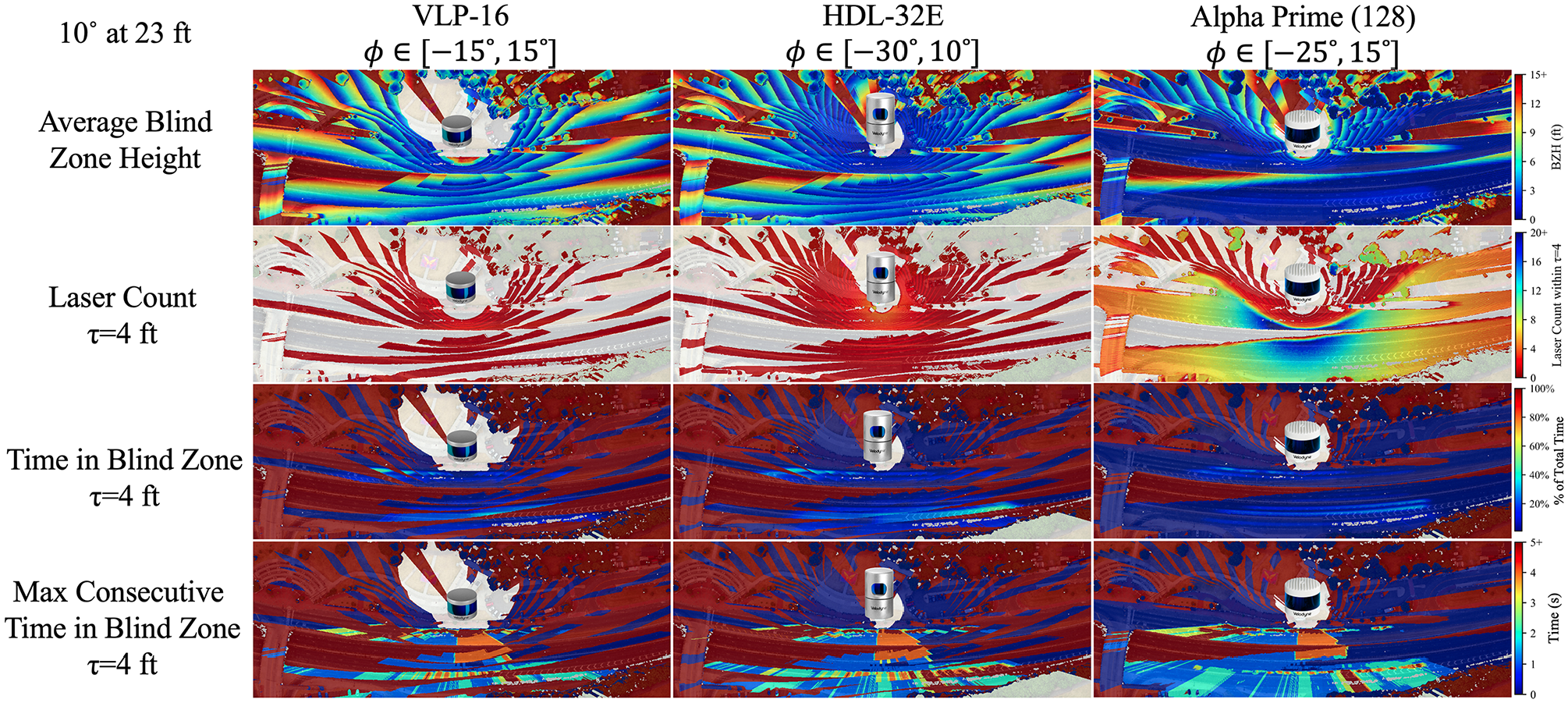
Average blind zone height, laser count, time in the blind zone, and maximum consecutive time in the blind zone of different light detection and ranging (LiDAR) devices.
Conclusions
This paper has presented an improved LiDAR blind zone evaluation model that simulates laser beams over a background generated using videogrammetry to evaluate and determine the optimal LiDAR configuration including six parameters: installation
With regard to applications, the inclusion of real-world background data allows for a meaningful evaluation of the blind zone with different LiDAR positions and angles. Trajectories help determine whether the blind zone affects traffic sensing. All simulation and evaluation results can be directly projected onto real-world coordinate systems such as NAD83 and WGS84, validated by generating 2D GeoTIFF images and importing them into ArcMaps. In addition to virtual LiDAR simulation for design, the real-world coverage map with the placement of actual LiDAR devices also allows geo-referenced LiDAR sensor search, which can speed up data query for specific incidents or accidents.
With regard to performance, to enhance efficiency in dynamic LiDAR blind zone simulation, we sampled the 3D background model into a DSM-like structure. We also proposed a new data structure that stores the occlusion status of each laser beam in each grid rather than in 3D space with accurate heights. This approach can save significant memory compared with traditional voxel-based structures, and even in comparison with the grid-laser-based structure from our prior paper, it saves seven times the memory for the structure when integrating LiDAR data with 3D models, such as in Digital Twin applications. At a resolution if 0.3 m, the sensor coverage analysis operates at approximately 53.35–58.97 Frames Per Second (FPS) for each 16-beam LiDAR device, 30.05–32.25 FPS for each 32-beam LiDAR device, and 8.25–9.36 FPS for each 128-beam LiDAR device, using a desktop with an Intel 13900KF CPU, 16 GB of 5,200 MHz DDR5 RAM, and an Nvidia RTX 3090 GPU. The processing involves updating the DSM to reflect dynamic traffic over a static background, determining the blind zone height, and generating the dynamic blind zone height results. Combining this with the 10 FPS frame rate of the Velodyne Alpha Prime and real-time edge processing at 10 FPS, the maximum system latency is expected to be less than 321 ms. This latency is calculated from the moment a road user appears to when the blind zone is modeled and analyzed, assuming that the processing units are on the same local area network that internal transmission time can be ignored. With 321 ms latency, a vehicle traveling at 40 mph can move 5.74 m between two frames. This can increase to 7.175 m at 50 mph, 8.61 m at 60 mph, and 10.045 m at 70 mph. In our experiment, the processed trajectory has an additional 0.11- to 0.15-s delay because of Internet transmission. The primary source of latency is the frame rate of the LiDAR devices. Unlike cameras, which can easily achieve 60 FPS or even 120–240 FPS, LiDAR devices typically operate at 5–20 rotations per second. Restricted by the implementation, the processing time with Python may not be competitive with more efficient code implemented in C++. The methodology proposed in this paper that uses a DSM-like structure for 3D analysis is theoretically computing more efficiently than voxel-based methods and has better robustness against an increasing number of road users compared with mesh-based methods.
With regard to validation, we propose two matrices to validate the generated DSM and one matrix to validate the simulated static blind zone with actual LiDAR data. With regard to evaluation, we updated two matrices from the prior paper and proposed one new matrix to evaluate the static blind zone affected by the background (terrain and infrastructures). We reapplied three matrices with new “in blind zone” determination criteria to evaluate the dynamic blind zone affected by traffic.
The DSM-based LiDAR 3D blind zone analysis model sacrifices actual 3D information in favor of computational and memory efficiency. As a trade-off, the model struggles to handle multilayered 3D environments, such as tunnels or bridges with under-bridge traffic. Although the road users placed on the DSM reflect 3D orientation based on each vehicle’s direction and the terrain, the model does not accurately account for the precise position of the four wheels. Consequently, it fails to capture vertical movements caused by small obstacles with accuracy. Another limitation is that the blind zone determination operates at the DSM resolution. For instance, if the DSM is sampled on a 0.3 m × 0.3 m grid, the vehicle will also be sampled at a resolution of 0.3 m to avoid unnecessary computational or storage costs caused by mismatched accuracies. For a site-specific blind zone analysis, a DSM-based background and actual trajectory data are generated and imported to assess the detection performance of using LiDAR devices on Route 18, NJ. The proposed model calculates the 3D blind zones based on the background (if provided) for static blind zones and traffic trajectories for dynamic blind zones. The output visualizes the 3D blind zones on 2D maps, color coded by different evaluation matrices, and projects the maps onto a real-world coordinate system (if applicable). In addition to the LiDAR point cloud data simulation, it not only shows the seen objects; the results also provide insights into what is really covered and what is not, even if no objects are seen. The optical geometry-based 3D SCM can be easily sampled at any resolution to match any background model. Thanks to the ease of creating a DSM background, the model can be transferred to evaluate the sensor blind zones on a virtual background generated for different scenarios.
The major blind zone findings include the following:
○ Height. The proper installation height for LiDAR sensors can help reduce occlusions and allow laser beams to penetrate gaps between vehicles. However, increasing the installation height comes at the cost of a larger blind spot directly below the sensor. ○ Angle. Tilting the LiDAR sensor effectively reduces the blind spot directly underneath the sensor and increases beam density near the LiDAR. However, excessive tilting can create new blind zones on the far side. ○ Position. Ideally, the sensor should be positioned as close to the road as possible. If large vehicles travel in the nearest lane, it may be beneficial to position the sensor slightly farther from the road.
○ Vertical FOV. The vertical FOV is important for roadside deployment. With a larger FOV downwards, the blind spot beneath the LiDAR will become smaller. Meanwhile, the LiDAR can be placed closer to the road. ○ Laser count. The lasers become sparse on distant objects. For roadside deployment, existing 16- or 32-beam LiDAR devices have no robustness against complex terrain, and the coverage is significantly impaired. But if the manufacturers can focus all the lasers from a 64-beam LiDAR downwards, it may maintain a good balance between cost and effective coverage.
○ Large vehicle. Higher and longer vehicles tend to create larger and longer-lasting blind zones. ○ Congestion. In light traffic conditions, blind zones are less frequent and severe. Congestion worsens dynamic blind zones because of increased traffic density and prolonged periods that grids that remain in blind zones. Sensor configurations should consider more severe blind zone situations during peak traffic hours rather than during free flow. ○ Terrain. Complex road terrain and infrastructure can cause significant static blind zones, making a multi-sensor setup necessary. ○ Surrounding. Small objects close to the sensor can create larger blind zones than large vehicles farther away. It is important to ensure that nearby devices do not obstruct the laser path between the LiDAR and the road/traffic.
Overall, it is generally advisable to increase the height to twice that of the tallest vehicle that may appear in the ROI. The resulting increased blind spot can be mitigated by adjusting the tilting angle, until the sparse upper lasers hit the road. When feasible, the sensor pole should be placed as close to the road as possible.
The exploration has been both interesting and challenging. Future work includes further refining the background model with trajectory data, evaluating the impact of additional weather and environmental factors, assessing the effect of system latency on safety-related applications, designing an efficient optimization method to fine-tune the six parameters for various objectives—such as maximizing detection coverage, maximizing 3D reconstruction coverage, and minimum costs with acceptable coverage trade-offs—and exploring the migration to on-board sensor coverage and camera coverage analysis. From a phased perspective, background model refinement and system latency assessment are short-term goals that depend on interdisciplinary expertise. In contrast, placement optimization for different tasks can be viewed as a long-term goal, requiring more efficient methods to analyze the overall impact of blind zones on traffic safety and to determine optimal configurations.
Footnotes
Acknowledgements
The corresponding author, Yi Ge, is deeply grateful to his wife, Yuting Wang, for her patience and support, especially during the revision process, which coincided with their honeymoon.
Author Contributions
The authors confirm contribution to the paper as follows: study conception and design: Peter J. Jin, Yi Ge; data collection: Yi Ge, Anjiang Chen; analysis and interpretation of results: Yi Ge, Peter J. Jin; draft manuscript preparation: Yi Ge, Peter J. Jin. All authors reviewed the results and approved the final version of the manuscript.
Declaration of Conflicting Interests
The author(s) declared no potential conflicts of interest with respect to the research, authorship, and/or publication of this article.
Funding
The author(s) disclosed receipt of the following financial support for the research, authorship, and/or publication of this article: This paper is based on work partially supported by Federal Highway Administration Research Project 21-60168, Middlesex County Resolution 21-821-R and the National Science Foundation under Grant No. 2133516. This paper is also partially based on work supported by the U.S. Department of Homeland Security under Grant Award 22STESE00001-03-02.
The views and conclusions contained in this document are those of the authors and should not be interpreted as necessarily representing the official policies, either expressed or implied, of the U.S. Department of Homeland Security.