
Abstract
During traffic data acquisition, missing data often arise owing to equipment failures and network disruptions. Despite extensive research on traffic data imputation, two primary limitations persist: First, existing methods struggle to fully integrate the spatiotemporal correlations and low-rank structures inherent in traffic data. Second, current research has mostly focused on missing completely at random (MCAR), with limited attention on other missing data patterns. We propose an innovative method, tensor completion and graph network fusion (TCGNF), to address these challenges for missing traffic data imputation. This method initially utilizes tensor completion for the preliminary imputation of missing data. Subsequently, it constructs the road network by leveraging the Pearson correlation coefficient from historical road data and the physical distances between detectors. The method then uses graph sampling and aggregation (GraphSAGE) to extract spatiotemporal data features from the two road networks and fuse them. Finally, these features are trained in generative adversarial networks (GANs) for accurate data imputation. Extensive experiments were conducted on two publicly accessible traffic datasets to validate the efficacy of the TCGNF model. The outcomes of these experiments indicate that the TCGNF model demonstrates superior generalization capabilities, significantly outperforming other state-of-the-art data imputation models concerning overall performance.
Keywords
Acquiring basic parameters such as traffic flow, speed, and density is crucial when planning, designing, and operating transportation systems ( 1 ). These elements significantly influence the efficiency and effectiveness of urban traffic systems ( 2 ). However, despite advances in data collection techniques, traffic information management systems in many countries still grapple with issues such as data corruption and loss ( 3 ). This persists as a significant challenge for intelligent transportation systems (ITS) ( 4 ). In traffic data applications, traffic data analysis algorithms such as support vector machines (SVM) and neural networks usually require complete datasets to improve prediction accuracy and make better decisions (5–7). Traffic data imputation algorithms have become a standard solution to cope with the problem of missing traffic data and to improve data integrity and availability ( 8 ). The application of this approach brings significant benefits to various stakeholders. For traffic management authorities, imputation algorithms can improve the accuracy of real-time monitoring so that traffic anomalies can be detected more quickly and effective emergency measures can be taken. This helps optimize resource allocation and improves the overall efficiency of traffic management. For city planners, relying on more accurate and complete data allows for more in-depth analyses of traffic patterns and infrastructure needs so that more efficient urban road networks and public transport systems can be designed to better cope with the growing traffic demand in the future. Traffic data imputation solves the challenge of missing data, empowers users to make more informed decisions, and supports the development of smarter, more efficient transportation systems.
Traffic data imputation has evolved from statistical models to deep learning methods ( 9 ). Statistical models primarily utilize basic statistical and mathematical models such as linear imputation and average estimation ( 10 ). Although these techniques are straightforward, they often overlook the complex relationships within the missing data, resulting in limited generalizability ( 11 ). As time series analysis methods developed, techniques like autoregressive integrated moving average (ARIMA) started to be used for traffic data imputation. While these methods enhance our understanding of data’s temporal dependencies, they exhibit limitations in managing nonlinear and non-stationary data ( 12 ). With the popularity of machine learning, techniques such as decision trees, neural networks, and SVM are effective in identifying complex relationships in data for traffic data imputation tasks, but this often relies on large parameters to the point of resource consumption ( 13 ).
In recent years, deep learning technologies have significantly propelled the field of traffic data imputation forward ( 14 ). For instance, while convolutional neural networks (CNN) are adept at learning local features, recurrent neural networks (RNN) and long short-term memory networks (LSTM) specialize in capturing temporal dependencies (15–17). Autoencoders have been effective in capturing low-dimensional structures ( 18 ). As a result, the precision of data imputation has experienced substantial enhancement ( 19 ). Furthermore, generative adversarial networks (GANs), which generate high-quality samples through adversarial training for traffic data imputation, have emerged as a primary research focus in recent years ( 20 ). At the same time, researchers are exploring the integration of deep learning models with other innovative technologies ( 21 ). For instance, integrating deep learning with graph neural networks (GNNs) and transfer learning has been under examination to harness additional a priori information ( 22 ). Ensemble learning frameworks are also being explored to combine the strengths of different models ( 23 ).
Despite the numerous solutions available for traffic data imputation, two primary limitations remain to be addressed.
First, existing methods often find it difficult to simultaneously consider the spatio-temporal characteristics of traffic data and its low-rank structure. However, traffic data have complex and variable spatiotemporal characteristics. For example, vehicles and pedestrians tend to be concentrated in office or recreational areas owing to the differences in functional attributes of different regions, which makes traffic data exhibit significant spatial correlation between regions. In the time dimension, the traffic patterns of morning and evening peaks are highly similar between days, and traffic flows are usually significantly correlated between neighboring periods or locations ( 24 ). In addition, there may be covariance in the data collected by different traffic detectors, which implies that the information from some detectors can be approximated by the data from other detectors, thus further highlighting the low-rank nature of the traffic data.
Second, many current methods are mainly designed for scenarios with missing completely at random (MCAR), making them less effective for other types of missing data. However, data missing in real-world traffic data are often not entirely random. For example, factors like unfavorable geographical conditions might result in devices in certain areas consistently being unable to gather data. This phenomenon can be categorized under spatially missing completely at random (MCARS).
This paper proposes an innovative approach to filling in the missing traffic data effectively and demonstrating good performance across different scenarios to address the problem of missing traffic data. For example, a city traffic monitoring system has missing data from some sensors owing to equipment failure or network problems, affecting monitoring traffic conditions at key intersections. By combining spatiotemporal correlation and low-rank structure imputation algorithms, the missing information is recovered using neighboring road sections and historical data, which helps the traffic management department monitor traffic conditions more accurately, identify potential congestion and optimize the emergency response, thus enhancing the efficiency of traffic management and citizens’ travelling experience. This approach can achieve effective imputation for both MCAR and MCARS, providing more accurate and comprehensive support for analyzing and applying traffic data. The contributions of this paper are as follows:
(i) A new deep learning framework is proposed to uncover the low-rank characteristics and complex spatiotemporal correlations within traffic networks and to accurately and robustly impute missing traffic data.
(ii) The preliminary imputation of traffic data using tensor completion is proposed. The preliminary imputation of the data by this mathematical method takes full account of the low-rank structure of the data itself. It lays a solid foundation for the accuracy of the spatial–temporal feature extraction of the subsequent data ( 25 ).
(iii) A new method for constructing temporal and spatial correlation road networks is proposed. The temporal and spatial correlation networks are constructed using the Pearson correlation coefficient and Gaussian function. The temporal correlation network reveals the correlation of traffic data between different time points, while the spatial correlation network shows the traffic flow patterns between different locations ( 26 ).
(iv) A spatiotemporal feature fusion method based on GraphSAGE is proposed. GraphSAGE is an efficient GNN algorithm that learns node embeddings without relying on global graph information ( 27 ). This method can better utilize the information from temporal and spatial-related road networks to extract more representative spatiotemporal features.
Related Work
The imputation of missing traffic data has been extensively studied, with various methods demonstrating strengths and limitations in handling spatiotemporal complexities. Tensor completion methods leverage the inherent low-rank nature of traffic data to achieve notable accuracy in data recovery but face challenges related to rank determination, outlier sensitivity, and scalability in dynamic scenarios ( 28 ). GNNs excel at capturing spatial dependencies in graph-structured traffic networks, enhancing imputation precision. However, their reliance on graph quality and limited capacity for modelling temporal dynamics pose challenges for large-scale, dynamic networks ( 29 ). GANs, particularly variants like Wasserstein GAN (WGAN), show promise in handling high-dimensional data distributions and improving training stability and imputation performance. However, they remain prone to mode collapse, sensitivity to architecture, and difficulties with spatiotemporal correlations ( 30 ). These limitations underscore the potential of hybrid approaches that integrate tensor completion, GNNs, and GANs, combining their strengths to address spatiotemporal challenges better and enhance the robustness and accuracy of traffic data imputation.
Tensor Completion
Tensor completion algorithms are techniques designed to impute missing values in multidimensional data ( 31 ). The core idea involves estimating missing values using low-rank matrices or tensor approximations ( 32 ). Given the inherent low-rank nature of traffic data, researchers have proposed a variety of tensor-completion-based methods for recovering missing traffic flow, speed, and trajectory data ( 33 ). These methods take full advantage of the low-rank structure of traffic data by designing matrix or tensor rank functions that can accurately describe its structure (34, 35). For example, in 2020, Chen et al. proposed a novel non-convex low-rank tensor completion (LRTC) model specifically designed to enhance the imputation of missing spatiotemporal traffic data. This model employs the truncated nuclear norm (TNN) minimization approach, which exhibits superior performance over existing methods, particularly in scenarios with high missing data rates. The LRTC-TNN model effectively captures and leverages the intrinsic low-rank structure of spatiotemporal traffic data, resulting in more accurate data imputation ( 36 ). By contrast, in 2022, Nie et al. introduced a method utilizing the truncated tensor Schatten-norm, aimed explicitly at efficiently addressing the complex missing patterns in spatiotemporal traffic data ( 37 ). The model efficiently addresses the non-convex optimization problem by integrating the alternating direction method of multipliers (ADMM) with the generalized soft thresholding (GST) technique. Furthermore, the study proposed a truncation rate decay strategy for different missing data scenarios, demonstrating through experimental results that the method achieves outstanding performance across various conditions. These methods have achieved satisfactory imputation effects when dealing with real traffic datasets.
Although tensor completion provides an efficient imputation scheme by exploiting the low-rank structure of traffic data, it still faces some challenges in practical application ( 38 ). For instance, the difficulty in precisely determining the rank of a tensor can lead to excessive or insufficient data imputation, and sensitivity to outliers may affect the model’s accuracy. Consequently, to improve the expressive power and usefulness of the model, further optimization of the use of tensor completion in traffic data imputation tasks is required. This includes developing more rationalized rank functions, strengthening the model’s resistance to anomalies, and adding outside data for supervision ( 39 ).
Graph Neural Networks
GNNs are a specialized category of deep learning models crafted for handling data structured as graphs ( 40 ). These graph-structured data don’t just encompass nodes (e.g., intersections, sensors in traffic networks) and edges (e.g., road segments, relationships between nodes): they also encapsulate the intricate interplay between these nodes and edges, which can include aspects such as the strength of connections, directional flows, or dynamic changes over time ( 41 ). Compared with traditional deep learning models, the uniqueness of GNNs lies in their ability to operate directly on graph structures, enabling them to effectively capture complex relationships and dependencies between nodes. For instance, in social network analysis, GNNs can be used to identify community structures; in molecular structure identification, they can predict chemical properties ( 42 ).
In traffic data imputation, GNNs analyze node data and capture node interactions within road networks. This dual capability enables more precise prediction and imputation of missing data. Particularly in complex or incomplete traffic networks, GNNs leverage information from adjacent nodes, enhancing the accuracy of data imputation by effectively mapping spatial relationships ( 43 ).
Considering specific applications, in 2022, Cini et al. introduced an innovative method termed the graph recurrent imputation network (GRIN) ( 44 ). This method, grounded in GNNs, addresses multivariate time series imputation. The essence of GRIN lies in its ability to reconstruct missing data within multivariate time series. This is achieved through the learning of spatiotemporal representations from sensor network data. Such an approach directly addresses the pervasive challenge of data incompleteness, especially evident in traffic network analysis.
GNNs also face several limitations in traffic data imputation. Their performance heavily relies on the quality of the graph structure, meaning inaccuracies in the adjacency matrix or relational definitions can degrade results. Additionally, for large-scale traffic networks, the computational complexity of graph networks poses challenges with reference to training time and memory consumption. Furthermore, while effective at capturing spatial relationships, graph networks often struggle to model temporal features adequately, limiting their ability to represent dynamic traffic patterns ( 45 ).
Generative Adversarial Network
GANs comprise two opposing networks: the generator, which produces refined samples iteratively to deceive the discriminator, and the discriminator, which determines whether a sample is actual or generated ( 46 ). GANs have demonstrated significant potential for traffic data imputation ( 47 ). GANs are more adept at grasping intricate high-dimensional data distributions than other deep learning frameworks. They can produce high-quality simulated data, effectively imputing missing information. For instance, in 2018, Yoon et al. introduced the generative adversarial imputation network (GAIN), which utilizes adversarial training for data imputation ( 48 ). In 2020, Chen et al. proposed a new method to enhance traffic data imputation through parallel data and GANs ( 49 ).
Early GANs employed the Jensen–Shannon divergence to measure the difference between the distribution generated by the model and the actual data distribution ( 50 ). Using this metric led to challenges in training stability, notably gradient vanishing and mode collapse. To mitigate these problems, Arjovsky et al. championed the WGAN, which adopts the Wasserstein distance over the Jensen-Shannon divergence ( 51 ). Adopting the Wasserstein distance has significantly improved GAN training stability. In traffic data imputation, WGANs have demonstrated superior performance ( 52 ). For instance, in 2022, Xu et al. employed a combination of WGAN and graph aggregators to address traffic data gaps effectively, demonstrating significant performance improvements ( 53 ).
While GANs hold promise for traffic data imputation, several limitations affect their effectiveness. The primary challenge is mode collapse, which can produce incomplete or repetitive imputed patterns, undermining result reliability. Additionally, GANs struggle to capture the temporal and spatial correlations essential in traffic data, and their training process is unstable and highly sensitive to architecture, hyperparameters, and loss functions, making generalization difficult across different datasets ( 54 ). Overcoming these issues requires refining network architectures, developing task-specific loss functions, and exploring hybrid models that integrate GANs with GNNs to capture spatiotemporal dependencies in traffic data better.
Method
Figure 1 illustrates the overall framework of the method proposed in this paper. It encompasses four main components. (1) Construction of two road networks: one based on temporal correlations derived from historical data and another based on spatial correlations from sensor distances. (2) Using the LRTC module for the preliminary imputation of missing data. (3) Extracting spatiotemporal features from the preliminarily completed data of the two road networks through GraphSAGE and fusion the spatiotemporal information of these two networks. (4) Using generative adversarial networks to achieve the final repair of network traffic data.
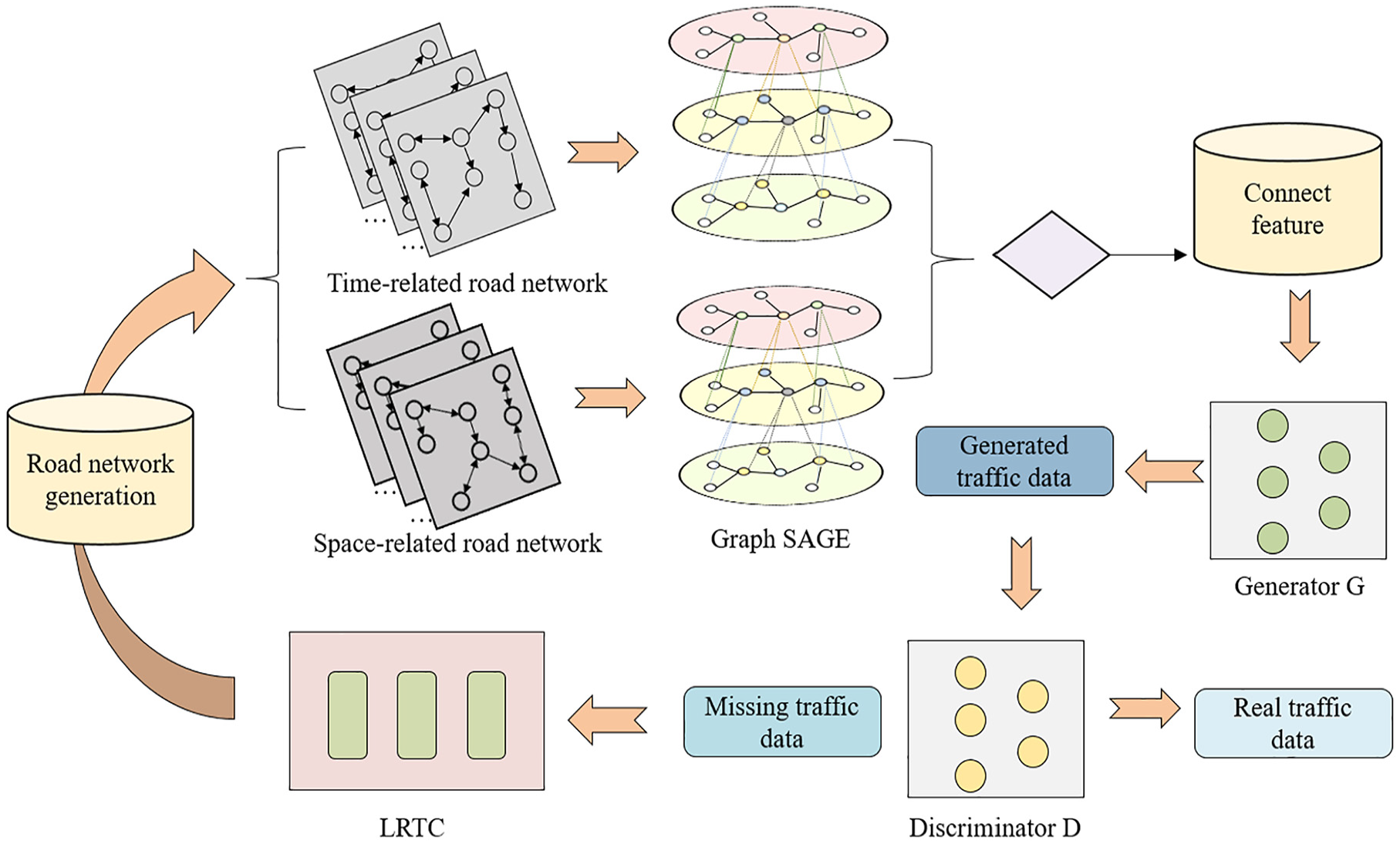
The structure of the tensor completion and graph network fusion (TCGNF).
Data Preprocessing
Firstly, the detectors in the road network are regarded as nodes of a graph
Next, based on the pattern of missing values in the traffic data matrix
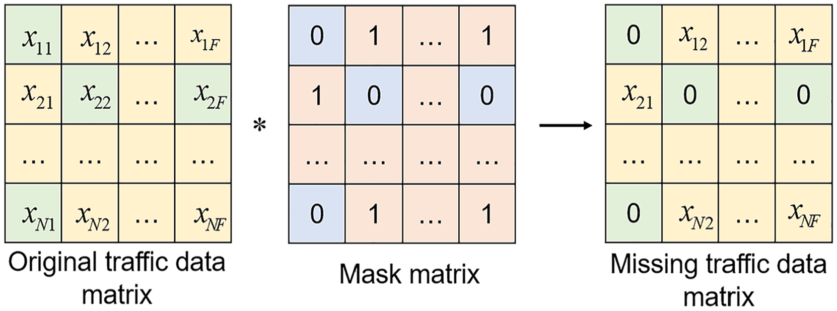
Missing data generation.
Road Network Construction
Construction of the Temporal-Correlation-Based Road Network
Using the Pearson correlation coefficient to calculate the temporal correlation between nodes in a road network is effective because it quantifies the linear relationship between traffic flow data at different time points. This method helps identify how traffic conditions at one node are related to those at another over time, capturing the temporal dependencies between traffic patterns at different locations. Given that traffic flow often follows linear trends over time, Pearson’s correlation is particularly suited for this purpose. The coefficient, ranging from−1. to 1, provides an intuitive and easily interpretable measure of correlation strength, facilitating the identification of significant temporal associations. Additionally, Pearson’s correlation is computationally efficient, making it highly suitable for large-scale traffic datasets and essential for reconstructing temporal correlation-based road networks in real-world applications.
For each road node i monitored by a detector, based on the historical traffic state data
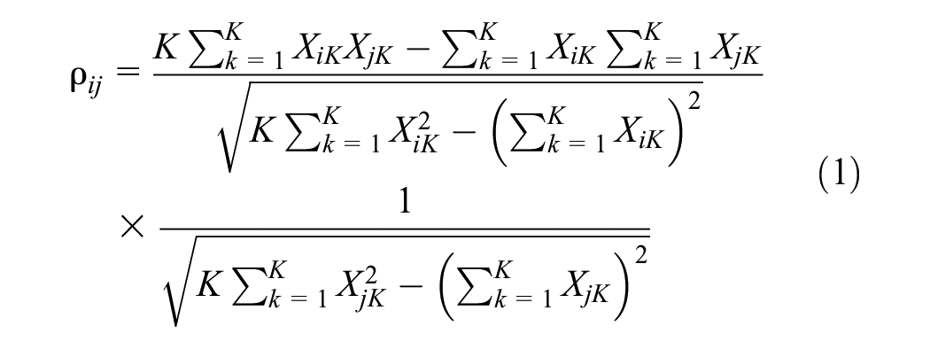
where K represents the length of the traffic network state nodes recorded by the selected detectors when calculating the Pearson correlation coefficient. Based on the calculated Pearson correlation coefficients, a Pearson correlation matrix
Some neighboring nodes have relatively low correlation with road nodes on the correlation coefficient matrix, which may interfere with the extraction of network features. To account for this, reconstruction of the traffic network involves selecting n detectors with higher Pearson correlation coefficients relative to node
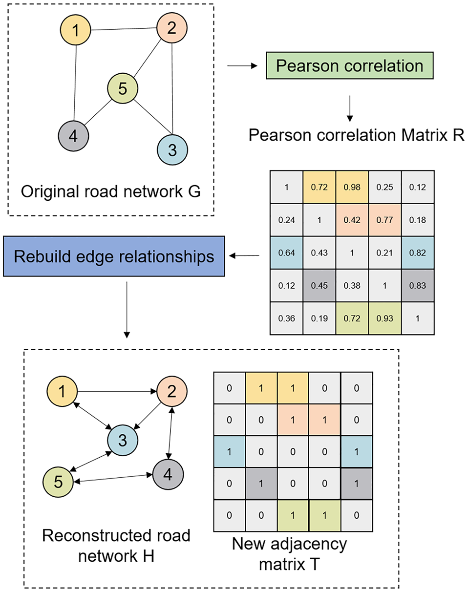
Construction of the temporal-correlation-based road network.
This method enables the identification of temporal associations between detectors within the original road network, thereby constructing a more correlated and accurate road network diagram. Although other methods, such as dynamic time warping (DTW), mutual information (MI), or even deep learning-based approaches, could potentially measure temporal associations, they often involve higher computational costs or added complexity. Compared with these alternatives, the Pearson correlation coefficient achieves a desirable balance between accuracy, simplicity, and computational efficiency, making it highly suitable for this study.
Construction of the Spatial-Correlation-Based Road Network
When considering the spatial relationships in sensor networks, traditional methods often limit their analysis to the direct physical connections between sensors. However, the indirect connections between sensors are particularly important in many scenarios, such as traffic monitoring or environmental surveillance. To more comprehensively reveal the network’s spatial relationships, this method proposes using a Gaussian function to construct an adjacency matrix that reflects the spatial relationships between sensors ( 55 ).
Initially, an adjacency matrix
The key step involves using a Gaussian function to convert each distance into a corresponding weight based on the standard deviation of the distance matrix, thereby reflecting the degree of interconnection between sensors in the network. The reason for using the Gaussian function is that it can smoothly decay the weights, making the closer sensors have stronger associations with each other, while the associations of the more distant sensors are gradually weakened, avoiding the phenomenon of abrupt changes in the traditional method, and also reflecting more accurately the natural spatial relationships between the sensors. The process is as follows:
Calculate the standard deviation σ of all non-infinite elements in the matrix

where μ is the mean of all non-infinite elements, and N is the number of non-infinite elements.
Transform distances into weights using a Gaussian function to obtain the weight matrix

This transformation reduces the impact of greater distances and normalizes the weights between 0 and 1. To decrease computational complexity and highlight closer spatial associations, the method adopts a similar construction approach to the temporal correlation matrix by selecting an appropriate n value, thereby increasing the sparsity of the matrix. The final output sparse adjacency matrix maps the physical distances between sensors and reveals their potential spatial relationships. This method makes it possible to understand and analyze the structure and function of sensor networks more precisely, providing a solid foundation for data processing and decision support.
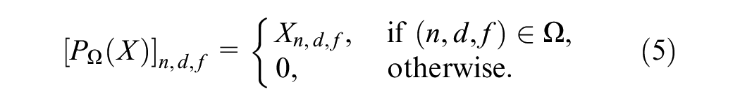
Low-Rank Tensor Completion
LRTC is a class of tensor completion methods based on the low-rank assumption. In this study, we apply LRTC for the initial imputation of traffic data. First, the missing traffic data
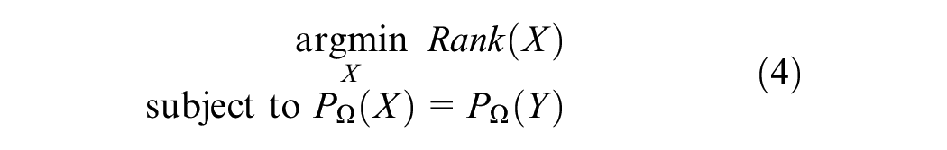
where
Here,
LRTC has several key limitations in traffic data imputation. First, rank minimization is an NP-hard problem, resulting in high computational cost, especially when handling large-scale, high-dimensional spatiotemporal data. Second, LRTC uses the standard nuclear norm (NN), which fails to distinguish between important and less significant singular values, potentially overlooking critical traffic patterns. Third, NN minimization can lead to over-smoothing, diminishing the representation of essential features, particularly in the presence of missing or noisy data. To address these issues, we introduce the TNN. By truncating smaller singular values and retaining larger ones, TNN effectively reduces computational complexity and improves data recovery accuracy. Moreover, TNN effectively prevents over-smoothing, significantly enhancing imputation performance, particularly in cases of missing or noisy data. The definition of the TNN regularization term is as follows:
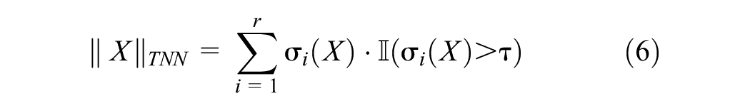
where X is the tensor, r is its rank, τ is a threshold parameter, and
Since the objective function minimized by TNN is non-convex, an ADMM-based non-convex optimization algorithm is employed. This algorithm decomposes the model optimization problem into three subproblems that are solved iteratively ( 56 ). This approach converts the original tensor completion problem into three subproblems that are solved iteratively.
Subproblem 1: Updating the tensor X
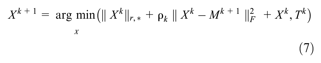
Subproblem 2: Updating the matrix M
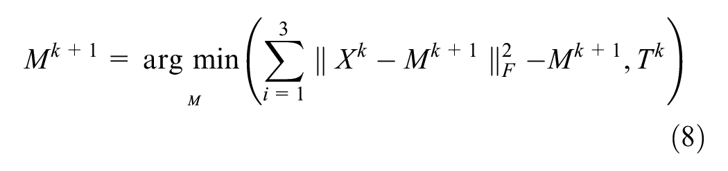
Subproblem 3: Update auxiliary variable T

where X is the current iterated data tensor,
These three subproblems collectively form the core optimization framework of the LRTC model. Solving these subproblems iteratively enables the model to converge toward an approximately completed tensor X, where missing values are imputed. This crucial step enhances the likelihood of having complete data available for the subsequent extraction of road network node features.
Road Network Feature Fusion
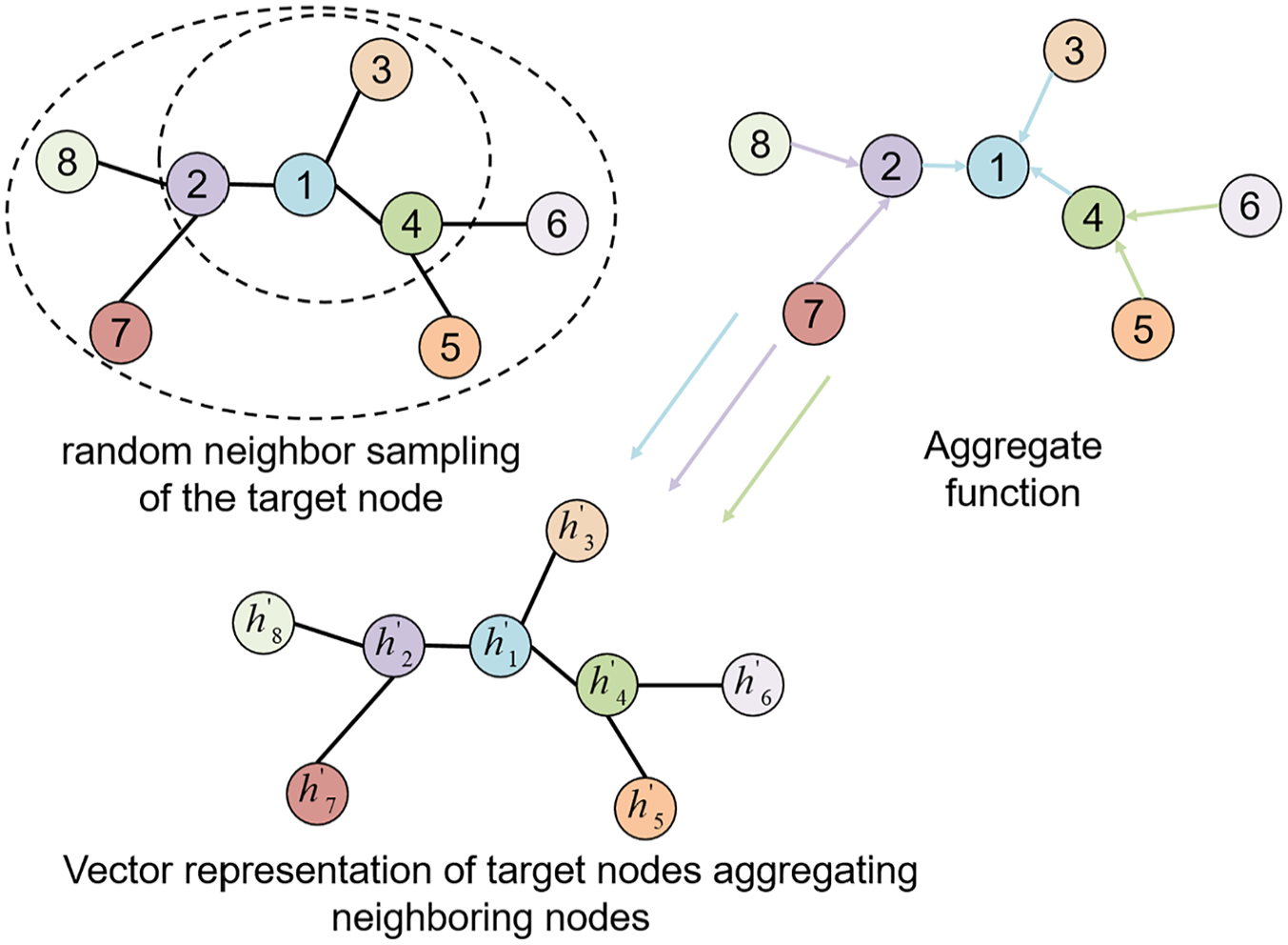
This study employs GraphSAGE to extract spatiotemporal information from reconstructed road network data, with the aim of improving the imputation of missing traffic data. The core of this method lies in how to aggregate feature information from neighboring nodes. The computation process can be divided into the following three steps:
Firstly, the adjacency matrix is processed to eliminate self-connections and normalize. This normalization ensures that the influence of each neighboring node is equal when aggregating their features. The purpose of normalization is to ensure that the aggregated features of each node are not biased by the differences in the number of neighbors.
Next, feature aggregation for the target node and its neighbors is performed using a selected aggregation function. Various aggregation functions are available, such as mean aggregation, LSTM aggregation, and pooling aggregation. This study selects mean aggregation, which calculates the average of each dimension across the embeddings of the neighboring nodes. The mean aggregation operation can be described as:

where Z represents the depth of aggregation,
Finally, the embedding features of the nodes are computed through nonlinear transformation operations. The formula for computing the node embedding features is:

where
Through Z layers of aggregation operations, we obtain the aggregated features for each node, which represent the road network’s features at different levels of abstraction. The node aggregation process is illustrated in Figure 4, where two layers of GraphSAGE are used to extract features from the road network nodes.
Node feature extraction.
After aggregating features from the spatially correlated road network data and temporally correlated traffic flow data to obtain

This concatenated feature vector
Generative Adversarial Network Training
The GAN, consisting of a generator and a discriminator, is employed to generate accurate traffic state data. The generator produces complete traffic state data by using the aggregated features of missing traffic state data. Simultaneously, the discriminator provides supervision to ensure that the distribution of the generated complete data is similar to the distribution of real data.
The training process of the generator and the discriminator relies on the definition of loss functions. The loss function of the generator consists of two parts: the loss from the discriminator on the generated data and the reconstruction loss. The reconstruction loss is used to measure the difference between the generated data and the real data. The generator consists of four linear layers, including three hidden layers and one output layer. The number of neurons in the hidden layers is 64, 128, and 256, respectively. After passing through the three hidden layers and an activation function, it takes an input and outputs the generated complete traffic state data. The generator’s loss function is as follows:

where
The discriminator in this study is symmetric to the generator and consists of four linear layers, including three hidden layers and one output layer. The number of neurons in the hidden layers is 256, 128, and 64, respectively. After passing through the output layer, a sigmoid activation function maps the output to a range between −1 and 1, representing the probability that the input data are real. The discriminator’s loss function consists of the loss from both the generated and real data. The discriminator’s loss function is as follows:

To address stability issues during the training process, this study employs WGAN. The training alternates between updating the generator and the discriminator, with the parameters of the discriminator being updated five times before updating the generator’s parameters to improve model convergence. The generator and the discriminator parameters are optimized using the Adam optimizer ( 57 ). This approach successfully implements data imputation for missing traffic data.
Experiment
Datasets and Data Configuration
This paper verifies the performance of, tensor completion and graph network fusion (TCGNF) on two real traffic datasets. Figure 5 shows the distribution of detectors across different datasets.
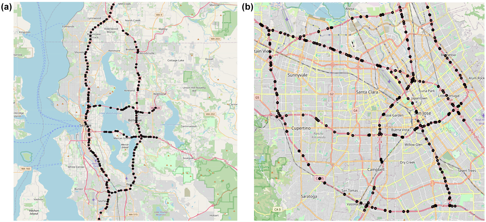
The distribution of detectors across different datasets: (a) Seattle Loop dataset and (b) PEMS-BAY dataset (PEMS-BAY—performance measurement system including data from the San Francisco Bay area.)
Seattle Loop Dataset: This dataset contains 2015 traffic speed data from 323 detectors along Seattle’s I-5, I-405, I-90, and SR-520 highways, recorded at 5-min intervals. Each detector provides time-stamped speed readings, structured as a time series with rows for time intervals and columns for individual detector readings (58, 59).
PEMS-BAY Dataset: Sourced from the performance measurement system (PEMS) by Caltrans, this dataset includes traffic speed data from 325 detectors across the San Francisco Bay Area, covering January 1 to June 30, 2017, at 5-min intervals. Similar to the Seattle Loop dataset, it provides time-series data with timestamps and detector-specific readings ( 60 ).
This paper proposes two missing data patterns: MCAR, where the probability of data being missing is completely independent of any other variable values, and MCARS, where the missing pattern is related to spatial, such as all data from a detector in a specific road segment being lost owing to a memory fault in the detector. The paper conducts experiments on data with missing rates ranging from 0.1 to 0.7 under these two patterns. Taking the PEMS-BAY dataset’s data from January 1, 2017, as an example, Figure 6 shows the heatmap of the complete data for January 1, 2017. The x-axis represents the time of the day (1/1/2017), and the y-axis represents different detectors.
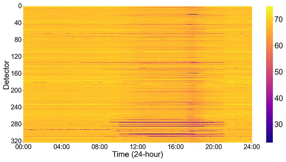
Heatmap of the PEMS-BAY observed data on January 1, 2017. (PEMS-BAY—performance measurement system including data from the San Francisco Bay area.)
Figure 7 displays the heatmaps for both MCAR and MCARS missing patterns at missing rates of 20%, 40%, and 60%. As the missing rate increases, the amount of zero data in the network grows, analogous to the increasing number of purple points in the heatmap.
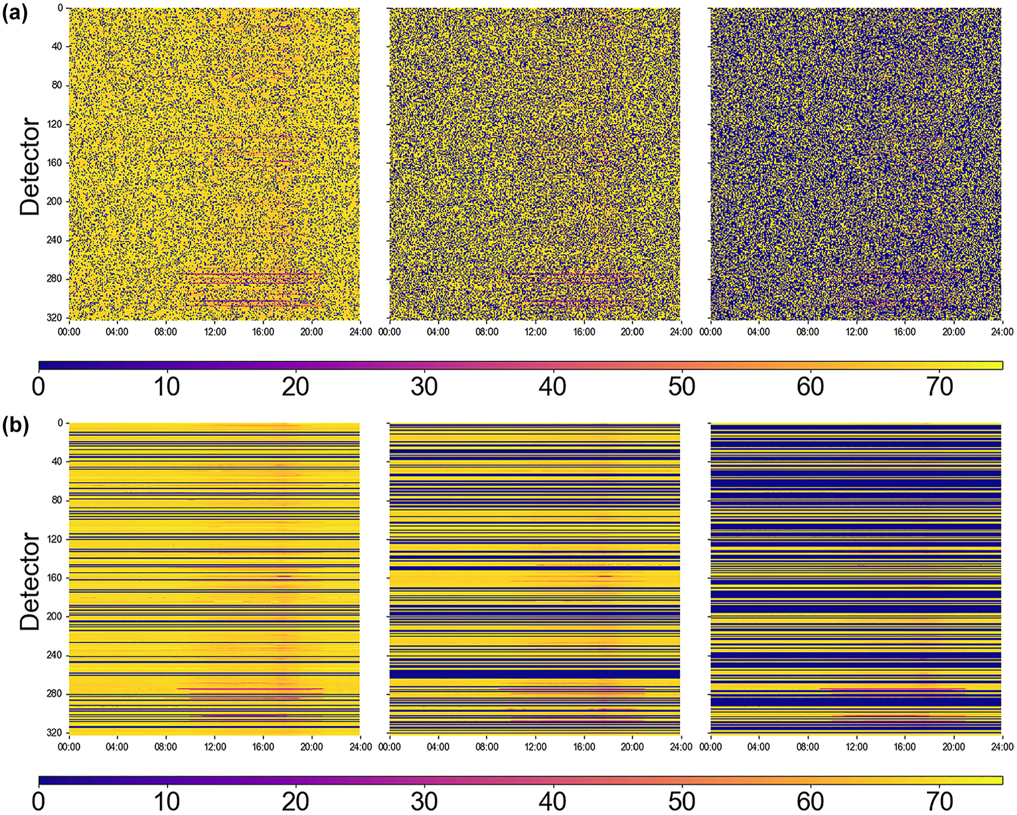
Heatmap of PEMS-BAY data on January 1, 2017: (a) missing completely at random (MCAR) missing patterns at missing rates of 20%, 40%, and 60% and (b) spatially missing completely at random (MCARS) missing patterns at missing rates of 20%, 40%, and 60%. (PEMS-BAY—performance measurement system including data from the San Francisco Bay area.)
Evaluation Metrics and Baseline Models
This paper employs three metrics for performance evaluation, including mean absolute error (MAE), root mean square error (RMSE), and mean absolute percentage error (MAPE). The calculation formulas are as follows:

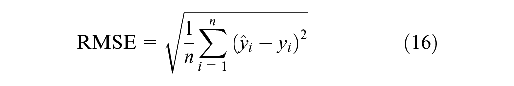

where
TCGNF is compared with the following representative baseline models:
(1) GAIN: A model that uses the generative adversarial network framework to generate and impute missing data, suitable for multivariate datasets ( 48 ).
(2) BGCP: A spatiotemporal traffic data imputation method based on Bayesian tensor decomposition, which enhances data integrity through Bayesian statistics and tensor decomposition techniques ( 61 ).
(3) LRTC-TNN: A non-convex low-rank tensor completion model utilizing truncated nuclear norm minimization, focused on addressing complex missing problems in spatiotemporal traffic data ( 36 ).
(4) LRTC-TSρN: Based on truncated tensor Schatten-norm, aimed at filling in complex missing patterns in traffic data ( 37 ).
(5) GA-GAN: A traffic state data imputation method based on graph aggregation generative adversarial networks, combining generative adversarial networks and graph aggregation technology ( 53 ).
(6) LCR: Combines circulant matrix nuclear norm with Laplacian kernel-based temporal regularization to efficiently impute traffic time series ( 62 ).
In TCGNF, the feature dimension
Experimental Results
The Experimental Results of the Seattle Loop Dataset
The selection of n values for the temporal-correlated and spatial-correlated networks was evaluated on the Seattle Loop dataset. The best performance was achieved with
Results of Different n in Temporal-Correlated Networks with 40% Missing in Missing Completely at Random
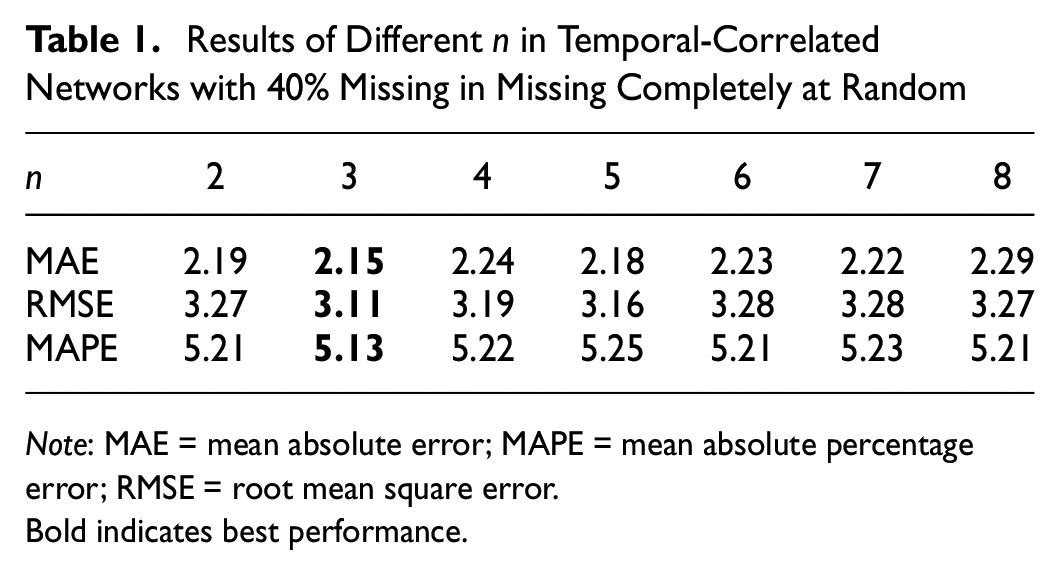
Note: MAE = mean absolute error; MAPE = mean absolute percentage error; RMSE = root mean square error.
Bold indicates best performance.
Results of Different n in Spatial-Correlated Networks with 40% missing in Missing in Missing Completely at Random
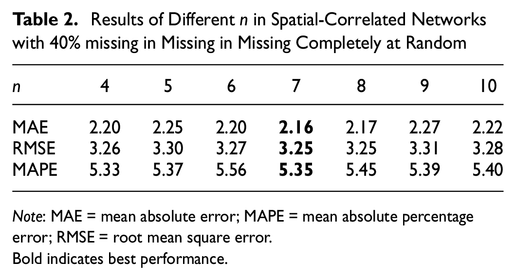
Note: MAE = mean absolute error; MAPE = mean absolute percentage error; RMSE = root mean square error.
Bold indicates best performance.
Figure 8 displays the distribution of residuals between the real data and the imputed data under different missing rates in the Seattle Loop. The left and right images in each subplot represent the residual distributions for the MCAR and MCARS missing patterns, respectively. At a 20% missing rate, the distribution of residuals in the MCAR pattern tends to be notably concentrated around the 0 value, and this concentration remains significant even when the missing rate is increased to 60%. From the MCARS pattern, it can also be seen that most residuals are near 0, indicating that the model can effectively identify different missing patterns and maintain its accuracy and robustness even at high missing rates.
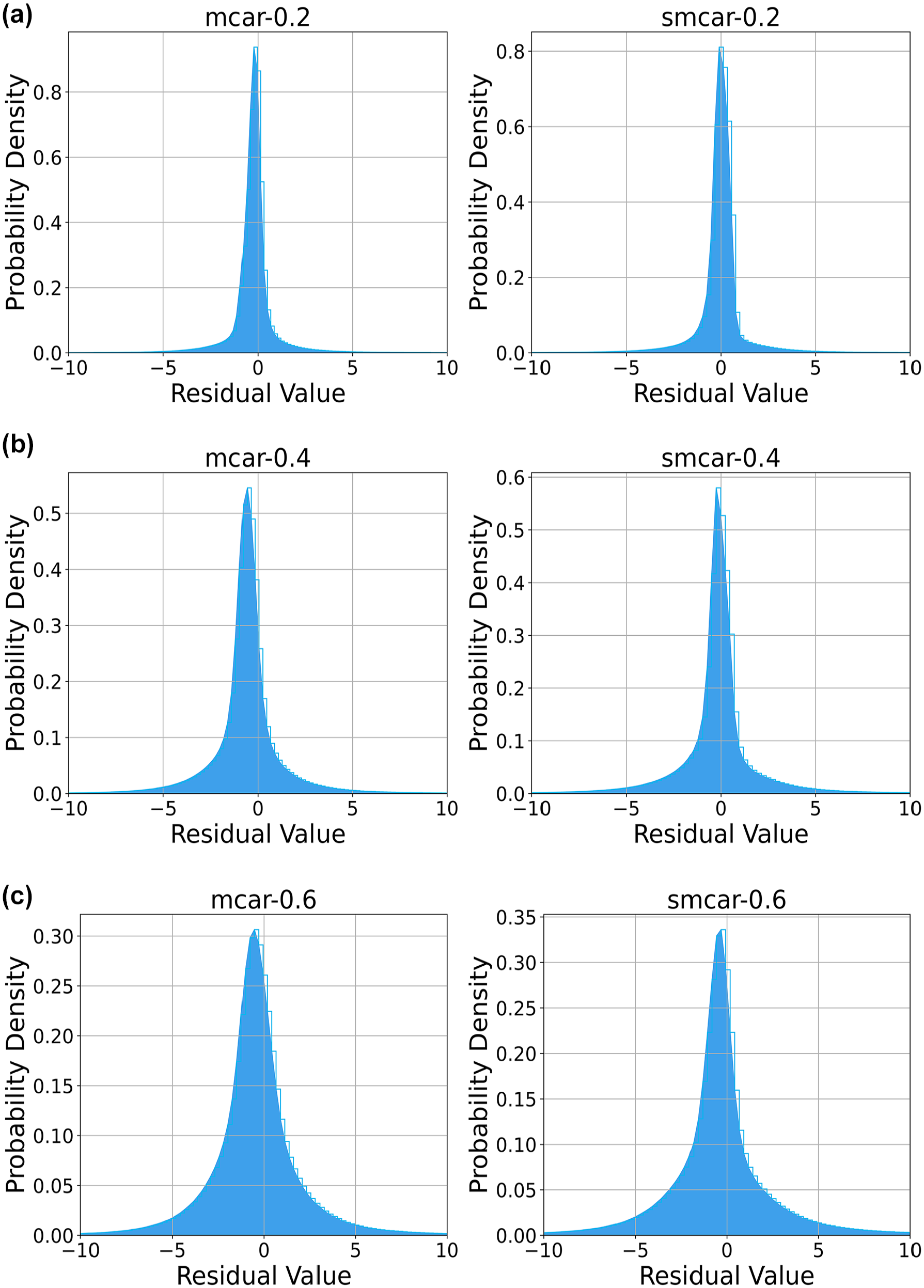
The residual distribution in the Seattle Loop dataset: (a) the residual distribution in the Seattle Loop dataset in the missing rate of 20%, (b) the residual distribution in the Seattle Loop dataset in the missing rate of 40%, and (c) the residual distribution in the Seattle Loop dataset in the missing rate of 60%.
Comparative experiments were conducted on the PEMS-BAY and Seattle Loop datasets under various baselines, missing ratios, and missing patterns. Table 3 presents the error metrics for the Seattle Loop data under the MCAR pattern, while Table 4 outlines the errors under the MCARS pattern. Both tables demonstrate that our model consistently outperforms the others across all patterns. Specifically, our model performs better than the LRTC-TSρN model in both the MCAR and MCARS patterns, with the LRTC-TSρN model being the best-performing baseline for comparison. In particular, under the MCAR pattern, our model achieves a MAPE significantly lower than 6.5%, and under the MCARS pattern, it remains below 10. While the GA-GAN model performs well under the MCAR pattern, its performance deteriorates under the MCARS pattern, where missing data are not completely random. Our analysis indicates that the GA-GAN model primarily relies on temporal correlation analysis within the network, but fails to sufficiently consider the low-rank structure of the data. This likely explains its weaker performance in addressing missing data at the spatial level. Additionally, the LCR model stands out as the second-best performer, after our model. However, owing to its reliance on a single low-rank tensor completion algorithm, it struggles with high missing rates, a limitation shared by other LRTC-based models. The LRTC-TNN and LRTC-TSρN models also exhibit similar issues, highlighting the significant performance degradation of low-rank tensor completion algorithms when faced with more complex missing data scenarios.
Error of Methods on Seattle Loop Data in Missing in Missing Completely at Random (MCAR) Pattern
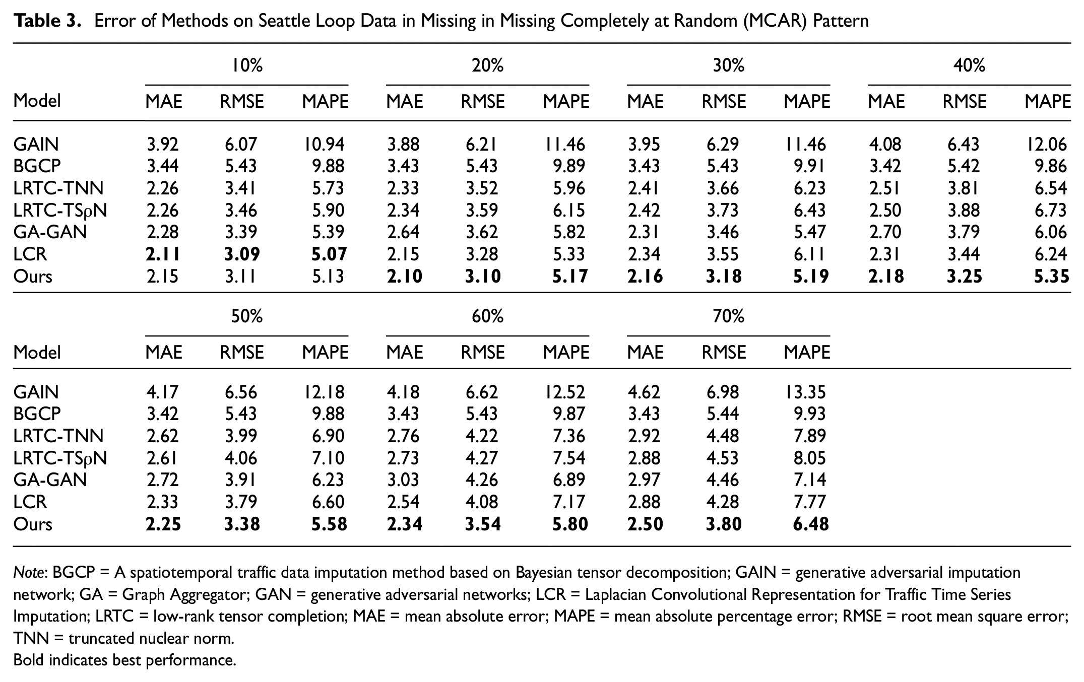
Note: BGCP = A spatiotemporal traffic data imputation method based on Bayesian tensor decomposition; GAIN = generative adversarial imputation network; GA = Graph Aggregator; GAN = generative adversarial networks; LCR = Laplacian Convolutional Representation for Traffic Time Series Imputation; LRTC = low-rank tensor completion; MAE = mean absolute error; MAPE = mean absolute percentage error; RMSE = root mean square error; TNN = truncated nuclear norm.
Bold indicates best performance.
Error of Methods on Seattle Loop Data in Spatially Missing Completely at Random (MCARS) Pattern
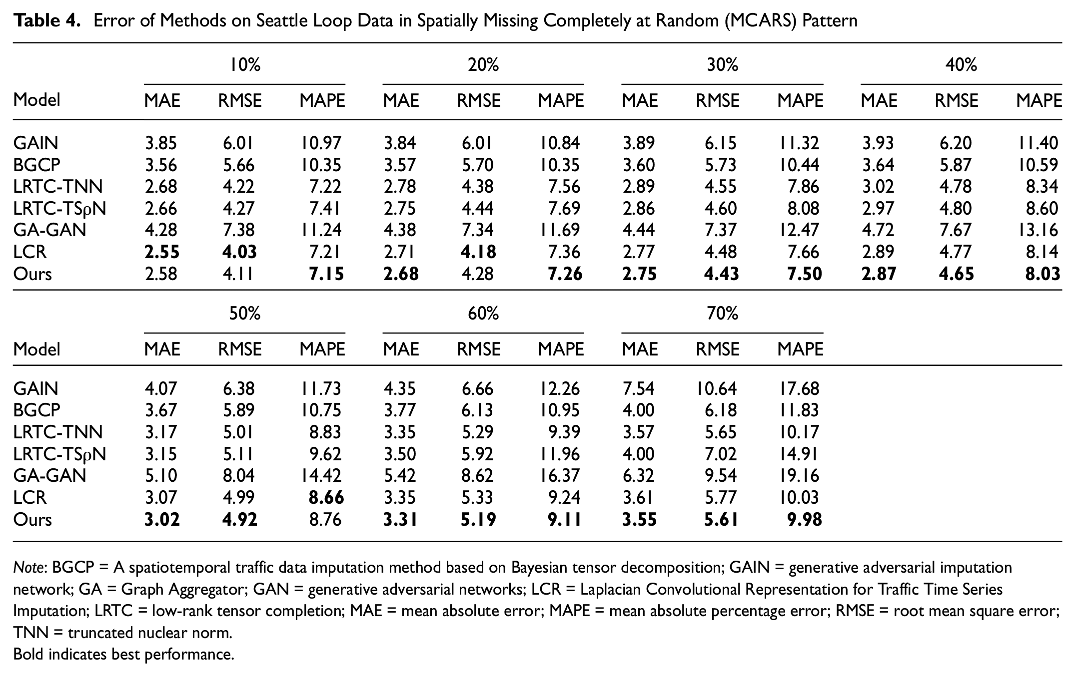
Note: BGCP = A spatiotemporal traffic data imputation method based on Bayesian tensor decomposition; GAIN = generative adversarial imputation network; GA = Graph Aggregator; GAN = generative adversarial networks; LCR = Laplacian Convolutional Representation for Traffic Time Series Imputation; LRTC = low-rank tensor completion; MAE = mean absolute error; MAPE = mean absolute percentage error; RMSE = root mean square error; TNN = truncated nuclear norm.
Bold indicates best performance.
The Experimental Results of the PEMS-BAY Dataset
Figure 9 presents the residual distribution in the PEMS-BAY dataset, where it is evident that the residual values cluster around 0, indicating the model’s exceptional performance on this dataset. Table 5 shows the error analysis for different missing ratios under the MCAR pattern using the PEMS-BAY dataset. In contrast, Table 6 displays the errors under the MCARS pattern. In both patterns, the TCGNF model demonstrated outstanding performance. Particularly in the MCAR pattern, the TCGNF model’s MAPE is below 2.4%, surpassing all comparison models’ best performance. Similarly, in the MCARS pattern, its MAPE remains below 5%, leading other models. It is worth noting that LRTC-TSρN performs better on the PEMS-BAY dataset because it has a larger dataset with clear spatial–temporal dependencies, which aligns well with the model’s low-rank assumption. In contrast, the Seattle Loop dataset, which consists of circular data from four interconnected highways, has a more complex spatial layout and traffic flow patterns, making it harder for the model to fully capture these intricate spatial–temporal relationships, leading to a lower performance. In all tested scenarios, whether compared with the PEMS-BAY or Seattle Loop datasets, TCGNF’s performance exceeds that of other comparison models.
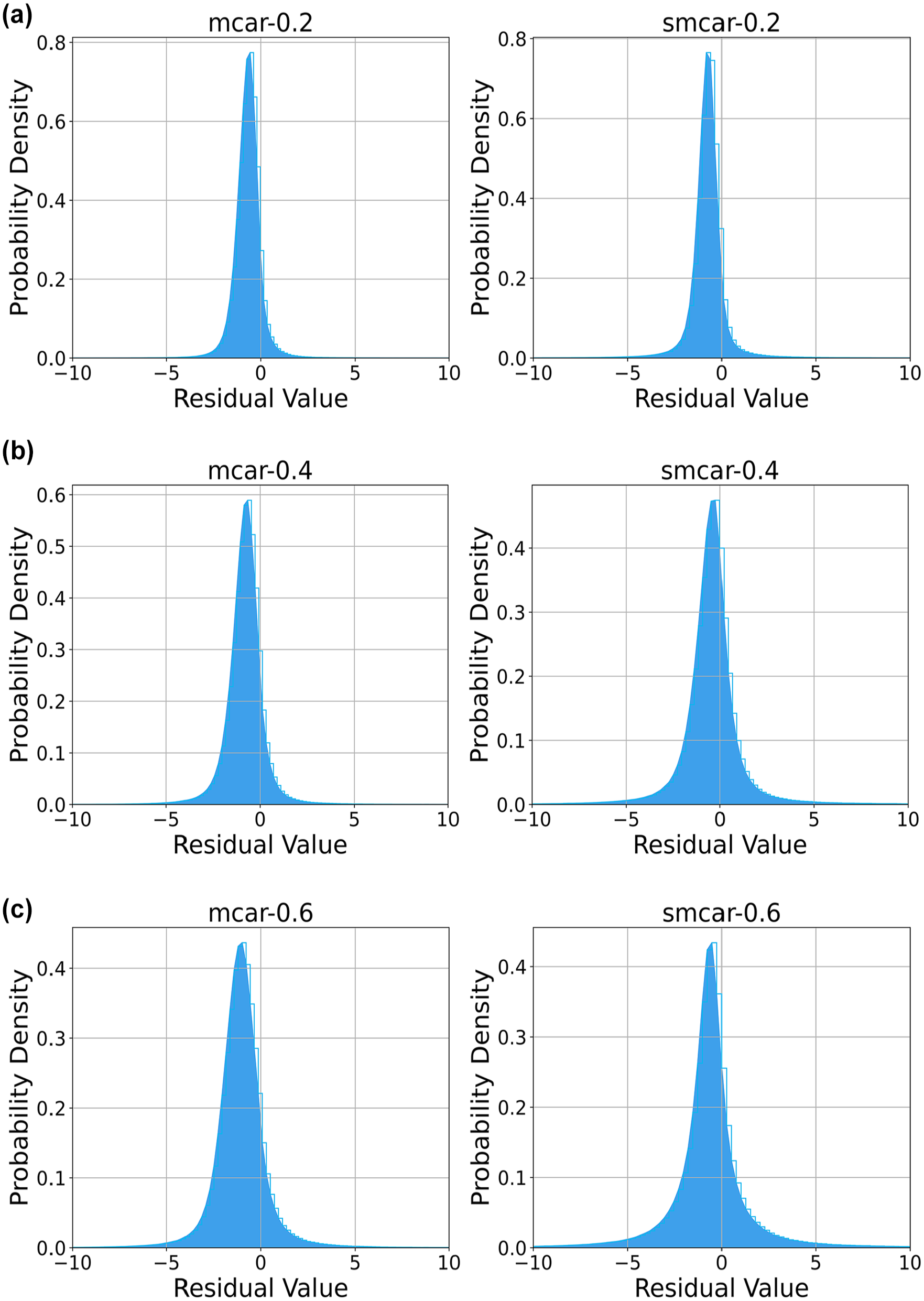
The residual distribution in the PEMS-BAY dataset: (a) the residual distribution in the PEMS-BAY dataset in the missing rate of 20%, (b) the residual distribution in the PEMS-BAY dataset in the missing rate of 40%, and (c) the residual distribution in the PEMS-BAY dataset in the missing rate of 60%. (PEMS-BAY—performance measurement system including data from the San Francisco Bay area.)
Error of Methods on PEMS-BAY Data in Missing Completely at Random (MCAR) Pattern (PEMS-BAY—performance measurement system including data from the San Francisco Bay area.)
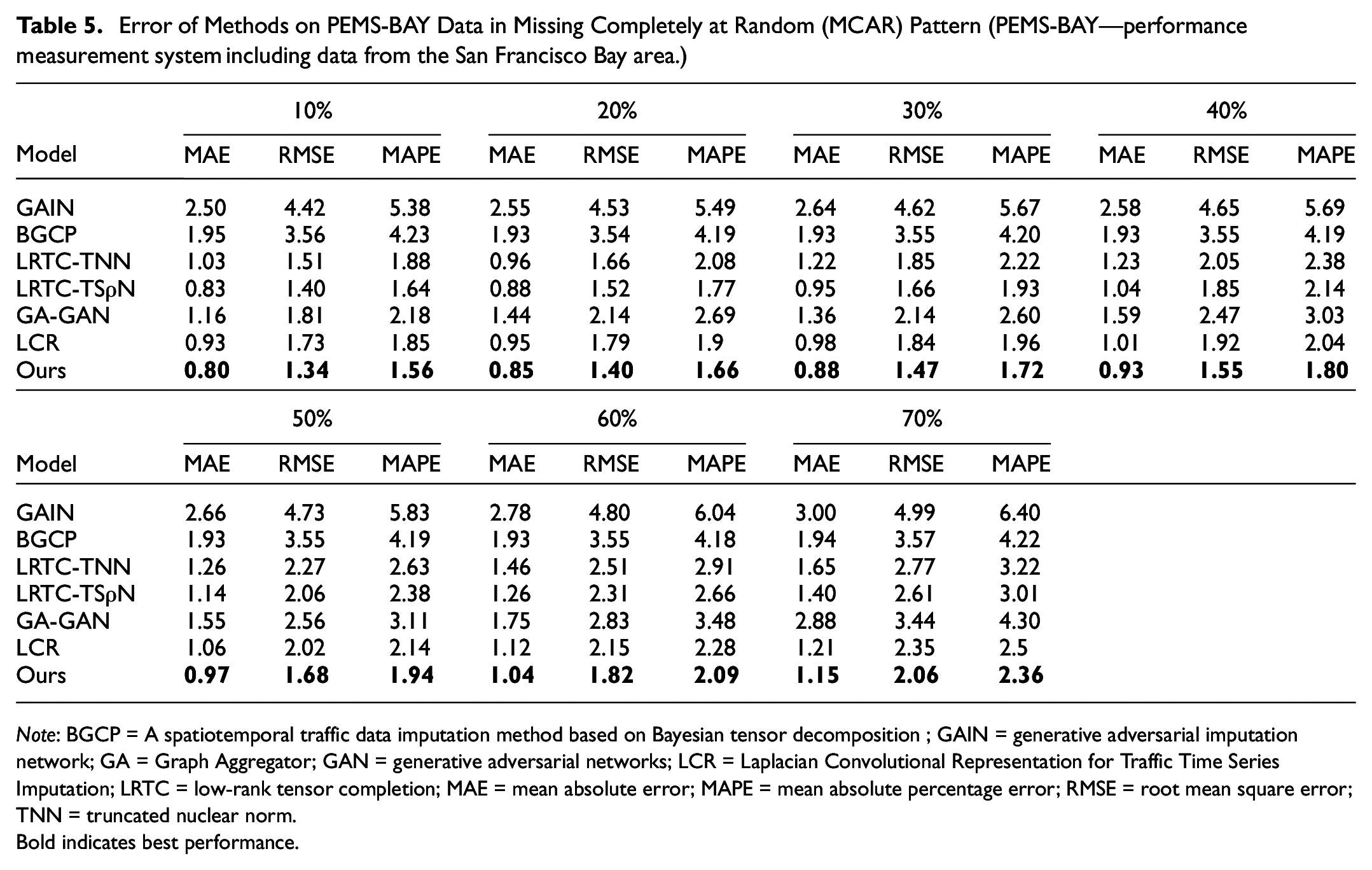
Note: BGCP = A spatiotemporal traffic data imputation method based on Bayesian tensor decomposition ; GAIN = generative adversarial imputation network; GA = Graph Aggregator; GAN = generative adversarial networks; LCR = Laplacian Convolutional Representation for Traffic Time Series Imputation; LRTC = low-rank tensor completion; MAE = mean absolute error; MAPE = mean absolute percentage error; RMSE = root mean square error; TNN = truncated nuclear norm.
Bold indicates best performance.
Error of Methods on PEMS-BAY Data in Missing Completely at Random (MCARS) Pattern (PEMS-BAY—performance measurement system including data from the San Francisco Bay area.)
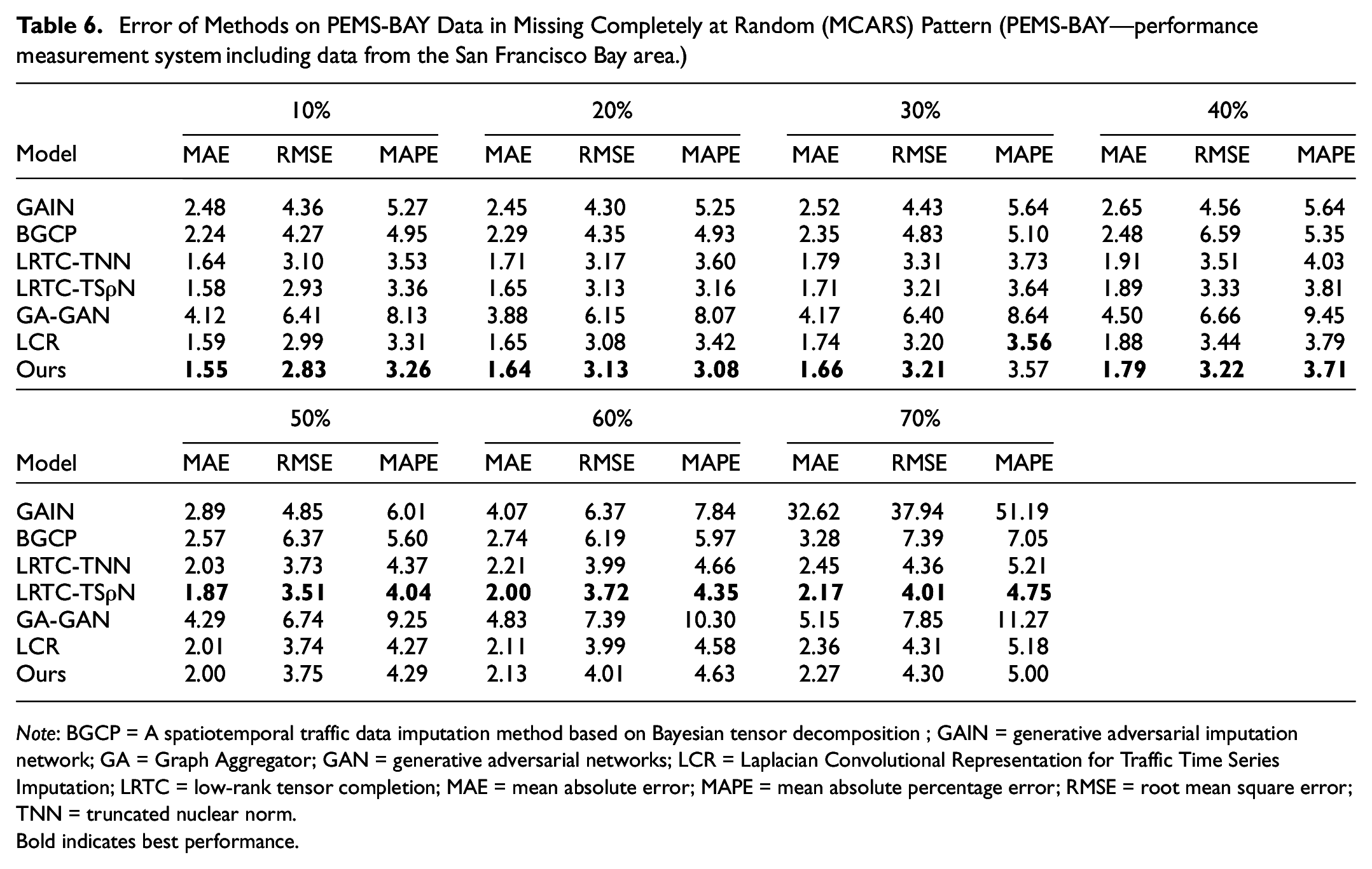
Note: BGCP = A spatiotemporal traffic data imputation method based on Bayesian tensor decomposition ; GAIN = generative adversarial imputation network; GA = Graph Aggregator; GAN = generative adversarial networks; LCR = Laplacian Convolutional Representation for Traffic Time Series Imputation; LRTC = low-rank tensor completion; MAE = mean absolute error; MAPE = mean absolute percentage error; RMSE = root mean square error; TNN = truncated nuclear norm.
Bold indicates best performance.
Ablation Experiment
This section aims to conduct ablation studies to show the contributions of different components within the proposed model. Given that MCAR is the most commonly studied missing pattern in the study, we conduct experiments under this pattern.
The Effectiveness of the LRTC Module
To verify the effectiveness of the LRTC module, two comparative experiments were set up: the first removes the LRTC module, and the second replaces the LRTC module with a basic moving smoothing completion module. The results are illustrated in Figure 10. Figure 10, a and b respectively, shows the comparisons for the Seattle Loop and PEMS-BAY datasets under the MCAR missing pattern. The x-axis of the graphs represents the missing rate, and the y-axis of the three subgraphs represent MAE, RMSE, and MAPE, respectively. “LRTC” indicates data preliminarily completed by the LRTC module, “SMOOTH” indicates data preliminarily completed by the moving smoothing completion module, and “NAN” indicates data without preliminary completion.
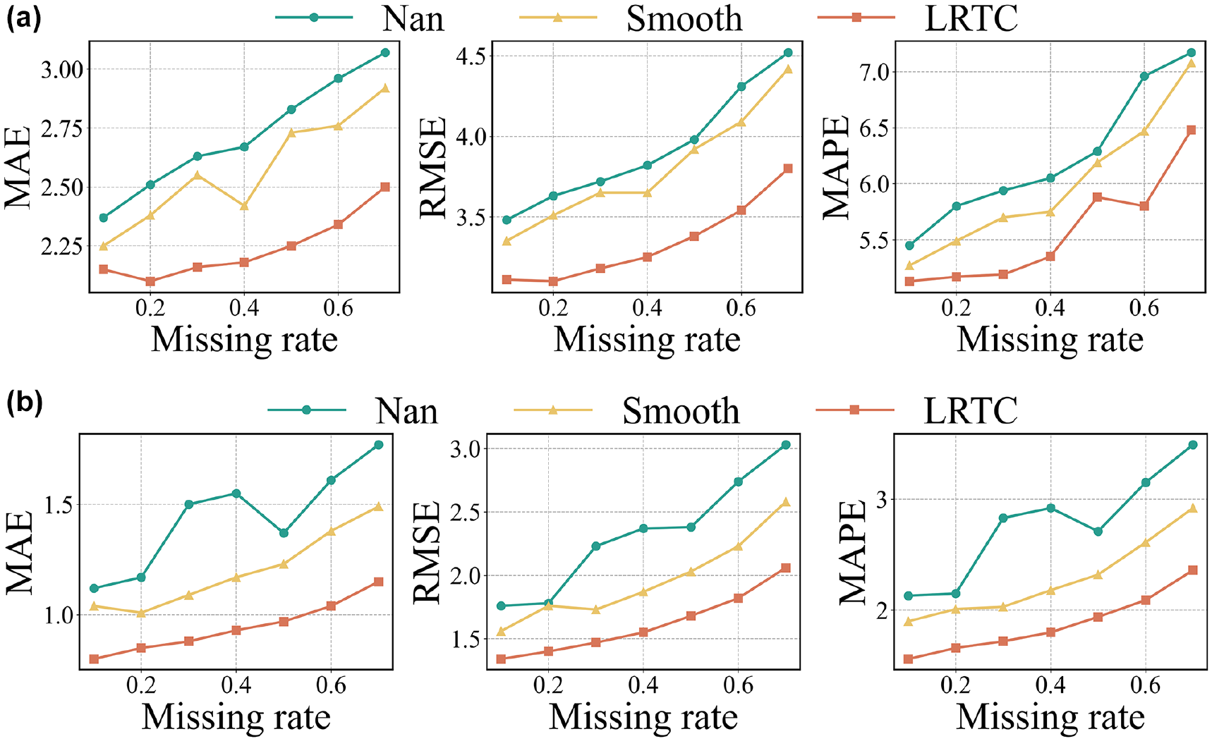
The effectiveness of the low-rank tensor completion (LRTC) module: (a) the effectiveness of the LRTC module in the Seattle Loop and (b) the effectiveness of the LRTC module in PEMS-BAY. (PEMS-BAY—performance measurement system including data from the San Francisco Bay area.)
The moving window step size for the moving smoothing completion was set to 3. In Figure 10, it is evident that the models which underwent preliminary completion using the LRTC module exhibit the lowest error values and the best imputation effects. The models that were preliminarily completed using the moving smoothing completion module ranked second, and the models without any preliminary completion performed the worst as regards imputation effectiveness. This demonstrates that LRTC preliminary completion is crucial in enhancing the model’s performance.
The Effectiveness of Road Network Fusion
To validate the effectiveness of network fusion, two comparative experiments were conducted: one using solely the temporal-correlation matrix for feature extraction and the other using only the spatial-correlation matrix for feature extraction. The results are illustrated in Figure 11. Figure 11, a and b respectively, shows the results of experiments on the two datasets. It can be observed that in the problem of traffic data imputation, spatial correlation has a greater impact than temporal correlation. The best imputation results are achieved when features from both are fused.
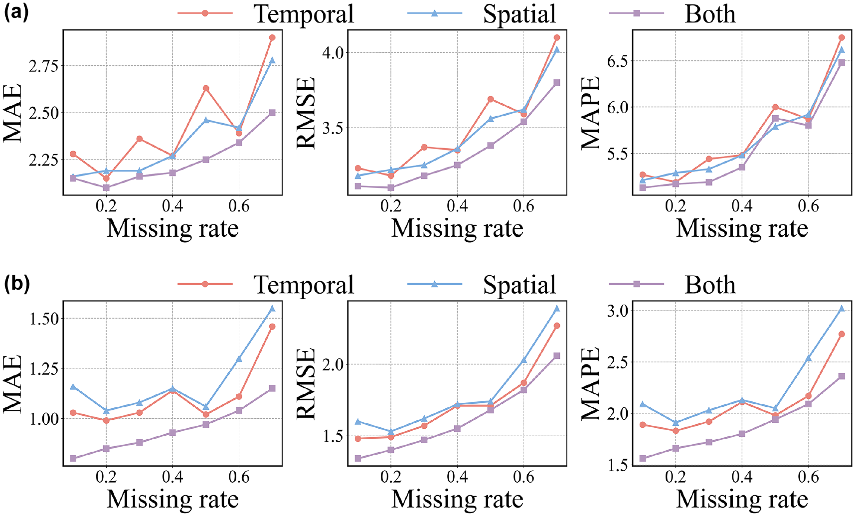
The effectiveness of road network fusion: (a) the effectiveness of road network fusion in the Seattle Loop and (b) the effectiveness of road network fusion in PEMS-BAY. (PEMS-BAY—performance measurement system including data from the San Francisco Bay area.)
Conclusion
This paper presents a novel approach for traffic data imputation, integrating tensor completion techniques with graph network fusion. We proposed a traffic state data imputation algorithm that leverages low-rank tensor completion, GraphSAGE feature fusion, and GAN. The algorithm begins by addressing missing data through low-rank tensor completion, followed by the construction of temporal and spatial correlation networks. Temporal correlations are calculated using the Pearson correlation coefficient, while spatial correlations are derived from the physical distances between detectors. GraphSAGE is then employed to extract features from these networks, optimizing the imputation process by effectively capturing the spatiotemporal dynamics of traffic data. Finally, GANs are used for model training, ensuring the generated imputed data reflect realistic traffic conditions. Experimental results on the Seattle Loop and PEMS-BAY datasets demonstrate the effectiveness of the proposed method, showing superior performance across various missing data patterns. The model successfully captures both the low-rank structure and spatiotemporal dependencies inherent in traffic data, significantly improving imputation accuracy. Despite these promising results, several avenues for future research remain. First, optimizing the method for computing temporal correlations between road networks, particularly by exploring alternatives to the Pearson correlation coefficient, could further enhance imputation accuracy. Second, while the approach has demonstrated effectiveness in traffic data imputation, its framework holds significant potential for generalization to other time series datasets, offering a versatile solution to missing data challenges across various domains.
Footnotes
Author Contributions
The authors confirm contribution to the paper as follows: study conception and design: Chengliang Xia, Xiang Yin; data collection: Junyang Yu, Xiaoli Liang, Lei Chen; analysis and interpretation of results: Chengliang Xia, Xiang Yin; draft manuscript preparation: Chengliang Xia, Xiang Yin, Junyang Yu. All authors reviewed the results and approved the final version of the manuscript.
Declaration of Conflicting Interests
The authors declared no potential conflicts of interest with respect to the research, authorship, and/or publication of this article.
Funding
The authors disclosed receipt of the following financial support for the research, authorship, and/or publication of this article: This work is partly supported by the National Natural Science Foundation of China (No. 42201465) and the Key Research and Development and Promotion Special Project in Henan Province (No. 232102210120, No. 232102211025).