Predicting and Evaluating Load-Displacement Trends of Helical Piles Using Machine Learning

Abstract

Evaluating the load-displacement trend of helical piles is essential to meet strength and serviceability standards for pile analysis and design. While pile load tests are the most accurate method, their cost and time constraints often lead in practice to the routine use of load transfer methods. This study aims to explore the feasibility of employing various machine learning–based algorithms to assess the load-displacement trend of axially loaded helical piles, using an existing database. Multiple machine learning models, including multi linear regression, K-nearest neighbors, random forest (RF), extreme gradient boosting (XGB), and artificial neural networks, were developed using data from 98 helical piles with a depth of 2.4 m to 16 m from 14 separate sites and corresponding in situ test data. Statistical evaluation was conducted to assess the performance of these models, comparing their predictions to measured curves from pile load tests. Based on the predictive analysis results, the average area under the regression error characteristic curve for XGB and RF was 0.035 and 0.043, respectively. The performance errors for XGB and RF were 0.01 and 0.05, respectively. The root mean squared error (RMSE) values for XGB and RF on the training data set were 0.083 and 0.1, respectively, while the RMSE values on the testing data set are 0.08 and 0.12.

Keywords

load-displacement trends axially loaded helical piles machine learning–based algorithms ultimate load-bearing capacity extreme gradient boosting random forest artificial neural networks

Pile foundations are essential for supporting structures on soft ground, transferring their weight deeper into the soil. Understanding how a single pile reacts to vertical loads is crucial for designing deep foundations, ensuring they meet both load-bearing and serviceability requirements. While pile load tests are the most reliable method, their cost and time constraints often limit their use to critical projects. Predicting pile load-displacement trends ( 1 – 3 ) through explicit modeling of construction processes is challenging and computationally intensive, hindering everyday application. Thus, the load transfer method, favored for its simplicity and feasibility, is widely used in practice. Load transfer methods are used to analyze helical piles and estimate their ultimate load-bearing capacity by modeling the distribution of forces between the pile and the surrounding soil. Two widely used approaches for load transfer analysis in helical piles are the cylindrical method and the single helix method, each offering distinct advantages depending on the pile configuration and soil conditions ( 4 – 6 ).

Helical piles, a widely employed foundation solution, have garnered significant attention in civil engineering because of their versatility and efficiency ( 4 ). Available methods for predicting the load-displacement behavior of helical piles rely on empirical equations and physical testing, which are fundamental to design and analysis. However, recent advances in machine learning–based algorithms (MLAs) could offer a supplementary tool for the preliminary evaluation of pile load behavior. Researchers have explored various MLAs such as multi linear regression (MLR), K-nearest neighbor (KNN), random forest (RF), XG Boost (XGB), and artificial neural networks (ANN) ( 7 ) to predict the load-displacement trends of helical piles ( 1 , 7 –9). By using large data sets and sophisticated algorithms, these studies aim to enhance the understanding and prediction capabilities of helical pile performance ( 10 ). MLR serves as a fundamental algorithm in machine learning, dating back to its introduction by Francis Galton in the late 19th century ( 11 ). Its simplicity offers users a transparent view of linear relationships within data, fostering confidence in accurate predictions. K-nearest neighbor (KNN), pioneered by Fix and Hodges ( 12 ), proves invaluable for both classification and regression tasks. Random forest (RF), stemming from the decision tree method and introduced by Breiman ( 13 ), aims to enhance prediction accuracy. XG Boost (XGB), presented by Chen and Guestrin ( 14 ), uses decision trees as base learners and has emerged as a widely embraced machine learning (ML) tool. ANNs mimic the structure and function of the human brain, featuring interconnected nodes or neurons that learn patterns through training. With versatility spanning classification, regression, and pattern recognition tasks, ANN offers a diverse array of applications.

In recent years, researchers have explored various machine learning algorithms (MLAs) to address a wide range of challenges in pile foundation design, achieving promising results ( 1 , 9 , 10 , 15 , 16 ). However, few studies have focused on predicting load-displacement curves for helical piles using MLAs, primarily as a result of the complexity of the input parameters. Identifying the most important parameters is challenging, which makes it difficult to develop a straightforward and accurate prediction method. A summary of selected related literature is presented in Table 1. For instance, Abu-Farsakh and Shoaib ( 3 ) assessed the load-settlement trend of axially loaded single square precast prestressed concrete piles using ML algorithms, specifically ANN, RF, and GBT to predict this trend from cone penetration test (CPT) data, including corrected cone tip resistance (qt) and sleeve friction (fs), using a database of 64 static pile load tests and corresponding CPT data. Ismail and Jeng; Ismail et al. ( 9 , 17 ) aimed to overcome the challenges of accurately estimating pile response to loading by developing a novel approach, employing a high-order neural network (HON) to simulate the pile load-settlement curve, using pile properties and standard penetration test (SPT) data as inputs and compared with methods such as backpropagation neural network, radial basis function, and general regression neural network models.

Table 1.

Selected Predictive MLA Used for Pile Evaluations

Reference	# of Piles	Pile type	# of train data (%)	# of test data (%)	Algorithms	Input parameters	Output parameter	Error metric	Error value
( 18 )	76	NA	85.60	14.40	ANN	SPT data	Displacement	RMSE	4.49
						Tip area
						Length
						Embedment depth
						Applied load
( 19 )	34	Drilled shafts	90	10	RNN	CPT data	Next load point	r	0.99
						Length		r	0.99
						Diameter		R²	0.97
						Previous load		R²	0.97
( 20 )	56	Concrete, steel, composite	90	10	ANN	CPT data	Displacement	r	0.96
						Loading type
						Pile material
						installation type
						Close or open-end		RMSE	4.34
						Cross section area
						Length
						Load
( 21 )	11	Bored	NA	NA	FTDNN	Length	Load	R²	0.99
						Diameter
						CPT data
					FFNN	Length	Load	R²	0.99
						Diameter
						CPT data
( 3 )	64	Precast prestressed concrete	90	10	ANN	CPT data	Load	RMSE	0.02
						Length
						Diameter
	64	Precast prestressed concrete	90	10	RF	CPT data	Load	RMSE	0.03
						Length
						Diameter
	64	Precast prestressed concrete	90	10	GBT	CPT data	Load	RMSE	0.02
						Length
						Diameter

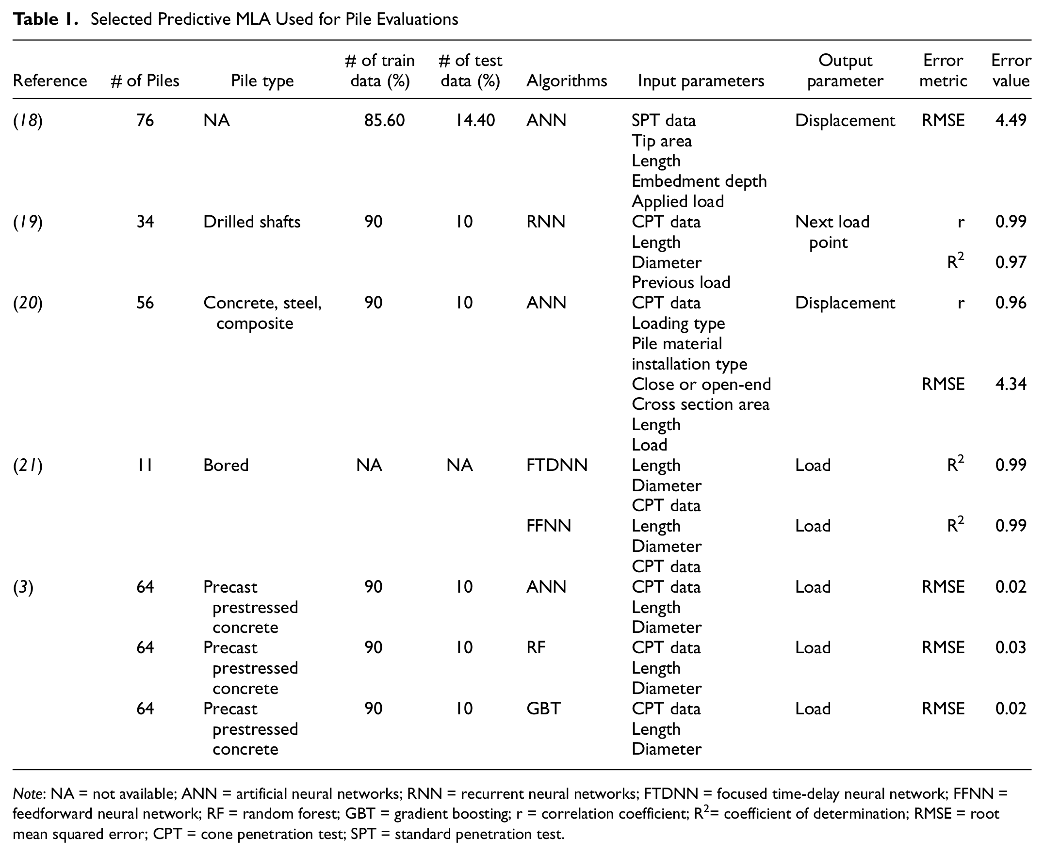
Note: NA = not available; ANN = artificial neural networks; RNN = recurrent neural networks; FTDNN = focused time-delay neural network; FFNN = feedforward neural network; RF = random forest; GBT = gradient boosting; r = correlation coefficient; R²= coefficient of determination; RMSE = root mean squared error; CPT = cone penetration test; SPT = standard penetration test.

The use of MLAs to predict the performance of piles has received increasing attention in recent years. Various studies have explored innovative approaches to predict pile capacity and improve prediction accuracy. Eslami et al. ( 1 ) investigated the potential of MLAs to predict the ultimate load-bearing capacity of helical piles. Their study evaluated multiple MLAs using a comprehensive data set to identify key features influencing pile performance, including geometric and soil parameters. The results demonstrated that MLAs, particularly ensemble methods, could achieve high prediction accuracy. Shuman et al. ( 10 ) explored MLAs for predicting the settlement behavior of large-diameter helical piles in c–φ soils. Their research emphasized the importance of input feature selection and highlighted the effectiveness of neural network architectures in capturing the nonlinear interactions between pile geometry, soil properties, and load-settlement behavior. Wang et al. ( 15 ) demonstrated the feasibility of using an ANN optimized with particle swarm optimization to predict the pullout bearing capacity of helical piles. Their study underlined the benefits of combining ANN with optimization techniques to enhance model accuracy and robustness, especially in scenarios with limited data. In another study, Wang et al. ( 16 ) evaluated MLAs for predicting the uplift behavior of helical anchors in dense sand for wind energy harvesting. By incorporating geometric and soil parameters, their research highlighted the efficiency of MLAs in modeling complex geotechnical behaviors, showcasing their potential for practical engineering applications.

Addressing the need for efficient and accurate methods to evaluate the load-displacement behavior of helical piles, this study aims to predict the load displacement of helical piles by implementing selected MLAs recommended in previous studies ( 1 ). The predictive models use data from 98 helical piles with a depth of 2.4 m to 16 m from 14 separate sites and corresponding cone penetration test (CPT) and standard penetration test (SPT) data. Recognizing the cost and time constraints associated with pile load tests, the research endeavors to harness the potential of MLA as a viable alternative.

Data Set

Description

To conduct this study, a total of 98 helical piles were carefully selected from the extensive database compiled by Rahimi ( 22 ). These selected piles were sourced from 14 distinct project sites located in Canada, the United States of America, South Korea, and Brazil. The selected helical piles exhibit a range of 1 to 6 helices, with helix diameters averaging between 254 mm and 762 mm, and installation depths varying from 2.4 m to 16 m. The specifications of these piles are presented in Table 2. Also, the distribution of the geometrical characteristics of the selected piles is illustrated in Figure 1 for visual reference and analysis. Please note that the water table as shown in Figure 1, represents the percentage of the pile depth that is submerged below the groundwater level.

Table 2.

Properties of Selected Helical Piles from the Database

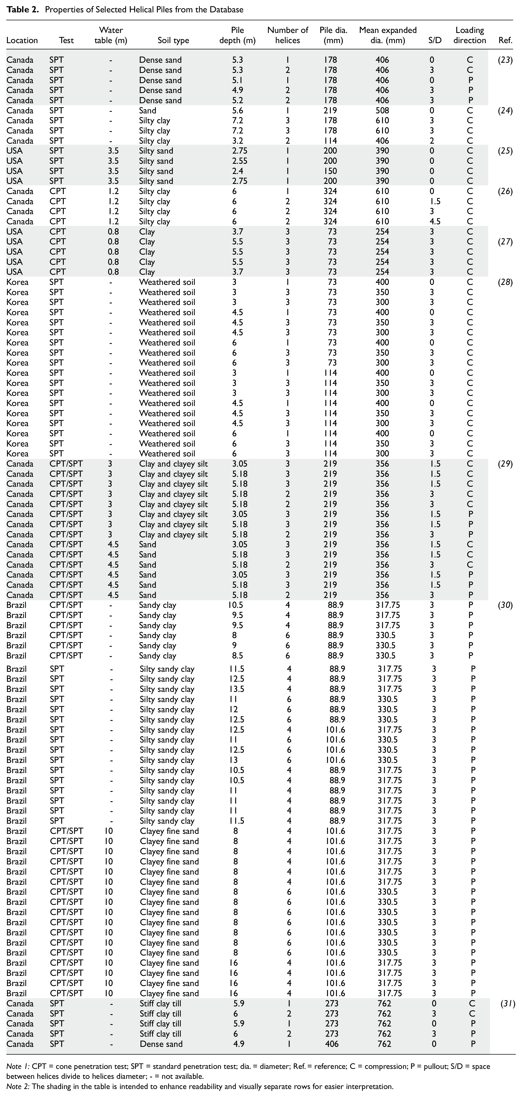
Note 1: CPT = cone penetration test; SPT = standard penetration test; dia. = diameter; Ref. = reference; C = compression; P = pullout; S/D = space between helices divide to helices diameter; - = not available.

Note 2: The shading in the table is intended to enhance readability and visually separate rows for easier interpretation.

Figure 1.

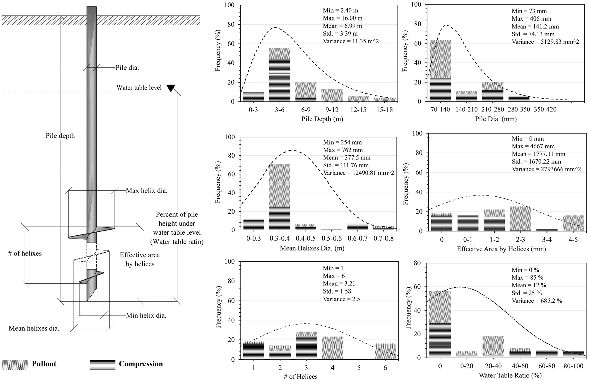
The database features the distribution of the helical piles.

Preparation

Calculate Ultimate Load

The ultimate load of each pile was used to normalize the load axis in the load-displacement curve. The criteria used for determining the ultimate load were the Brinch-Hansen 80% and an equivalent load with a displacement equal to 5% of the mean helices’ diameter. In cases where the ultimate load could not be calculated using the Brinch-Hansen 80%, the 5% criterion was employed. Figure 2 illustrates the overall scenario of the ultimate load calculated for each case in the database in comparison to the maximum measured load.

Figure 2.

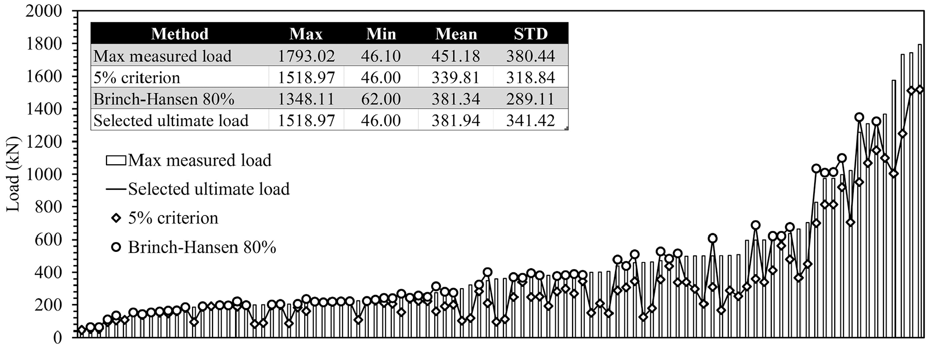
Helical piles ultimate loads in comparison to the maximum measured load.

While it may seem counterintuitive to compare piles with ultimate loads ranging from close to 0 to nearly 1,800 kN, this broad spectrum of pile capacities reflects the diversity in the data set. The inclusion of piles with widely varying ultimate loads is intentional, as it ensures the robustness and generalizability of the ML models used in the study. It is important to highlight that all input data, including ultimate loads, are normalized before being used to train the models. This normalization process effectively reduces the impact of variations in scale and magnitude across the data set. By doing so, the models focus on learning the underlying patterns and relationships rather than being influenced by the absolute differences in values. Additionally, the diversity in the data set enhances the models’ capability to make accurate predictions across a wide range of scenarios, which often involve varying pile and soil conditions. Figure 2 serves to illustrate the range and distribution of ultimate loads in the data set, highlighting the data that contributes to the reliability of the developed models.

Load-Displacement Curves Normalization and Model Framework

To accurately predict the load-displacement curve for helical piles, the displacement parameter was included as an input feature, representing the known values at different load stages. The corresponding load values for each displacement were treated as the target output for the ML algorithm to predict. This approach allows the model to learn the relationship between load and displacement effectively. For normalization, the load values were normalized with respect to the ultimate load, while displacement values were normalized using three key geometric parameters: pile depth (pile embedment), pile diameter (shaft diameter), and mean helices diameter. This normalization ensures that the model training process is not biased by the scale of the raw data and captures the critical influence of pile geometry on the load-displacement relationship. The trained model was then tasked to predict the load-displacement curve for a new pile, where displacement values (normalized using the same parameters) were provided as input, and the corresponding load values were predicted as output. The load-displacement curves for these data sets are depicted in Figure 3.

Figure 3.

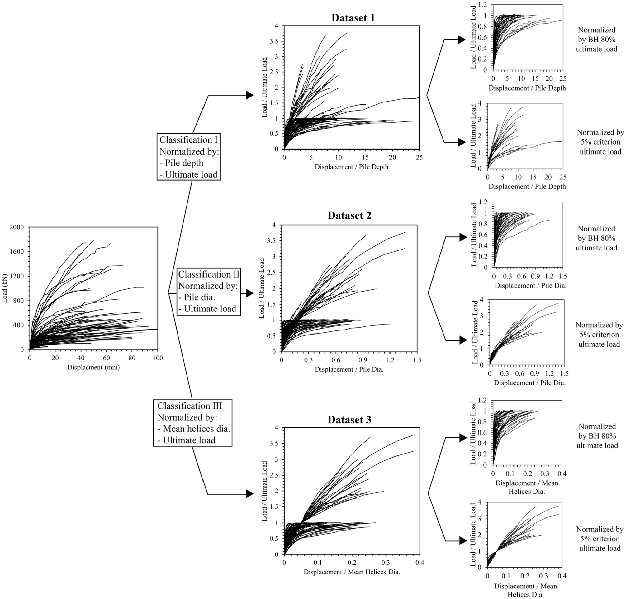
Helical piles load-displacement curves for different classifications for predictive model input normalization.

Soil Properties

The data on helical piles in the database can be classified into two main categories: geometric characteristics of the piles and soil properties. With regard to soil characteristics, SPT number values were frequently used as a key feature for training algorithms based on the available data and the prevalence of SPT in the field. In cases where only CPT logs were accessible, they were converted to SPT values to increase the data set. The relations used for this problem are presented in Table 3. Table 3 presents a series of equations (Equations 1 to 6) used to convert CPT data into equivalent SPT values, a necessary step since our models primarily rely on SPT values to characterize soil conditions. Furthermore, the water content at the depth where the piles were embedded was also considered a significant soil characteristic in the analysis.

Table 3.

Selected Correlations for Soil Layering Classifications (Convert CPT Data into Equivalent SPT)

Equation	Description	Ref.
$N_{60} = \frac{K_{h} K_{b} K_{s} K_{r} N}{60}$ (Equation 1)	$N_{60} Standard penetration number$ $corrected for field conditions$ $N Measured penetration number$ $K_{h} Hammer efficiency$ $K_{b} Correction for borehole diameter$ $K_{s} Sampler correction$ $K_{r} Correction for rod length$	( 32 , 33 )
$q_{t} = q_{c} + u_{2} (1 - a)$ (Equation 2)	$q_{c} : Cone resistance$ $q_{t} : Corrected coneresistance$	( 34 )
$Q_{t} = \frac{(q_{t} - σ_{v 0})}{σ'_{v 0}}$ (Equation 3)	$q_{c} : Cone resistance$ $q_{t} : Corrected coneresistance$ $Q_{t} : Normalized coneresistance$ $σ_{v 0} : In - situ vertical stresses$	( 34 )
$F_{r} = \frac{f_{s}}{(q_{t} - σ_{v 0})} \times 100 %$ (Equation 4)	$F_{r} : Friction ratio$ $q_{t} : Corrected coneresistance$ $σ_{v 0} : In situ vertical stresses$ $f_{s} : Sleevefrictionresistance$	( 35 )
$I_{c} = {(\begin{matrix} {(3.47 - \log Q_{t})}^{2} + \\ {(\log F_{r} + 1.22)}^{2} \end{matrix})}^{0.5}$ (Equation 5)	$Q_{t} : Normalized coneresistance$ $I_{c} : Radius of essentially concentric$ $circles that represent the boundaries$ $between each SB T_{n} zone$ $F_{r} : Friction ratio$	( 36 )
$\frac{(q_{t} / P_{a})}{N_{60}} = 10^{(1.1268 - 0.2817 I_{c})}$ (Equation 6)	$q_{t} : Corrected coneresistance$ $P_{a} : Atmosphere pressure$	( 29 )

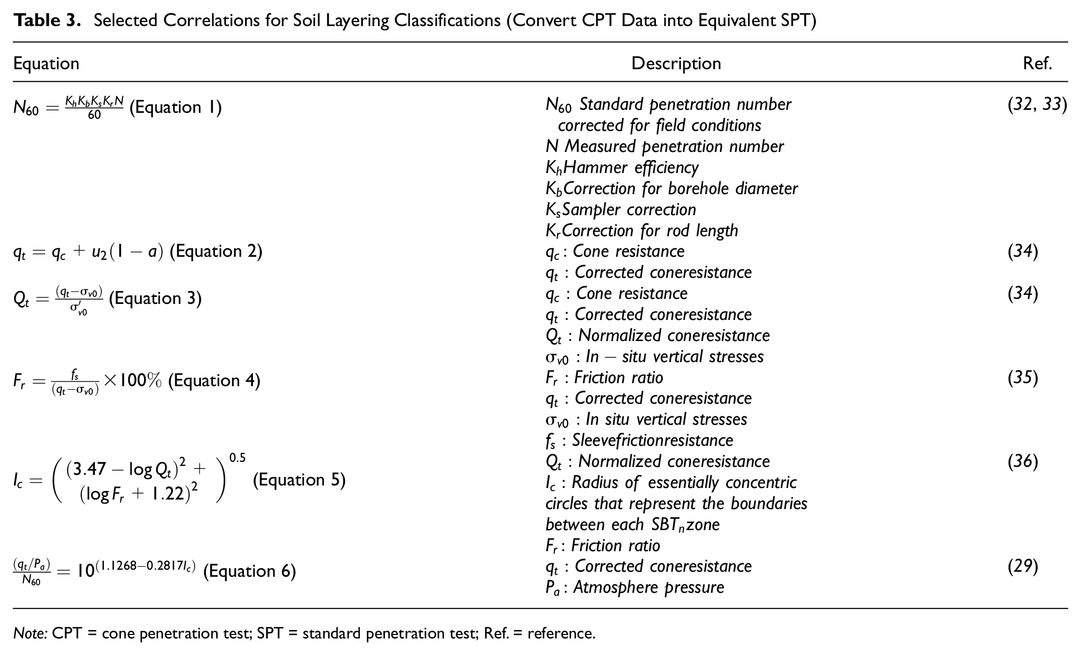
Note: CPT = cone penetration test; SPT = standard penetration test; Ref. = reference.

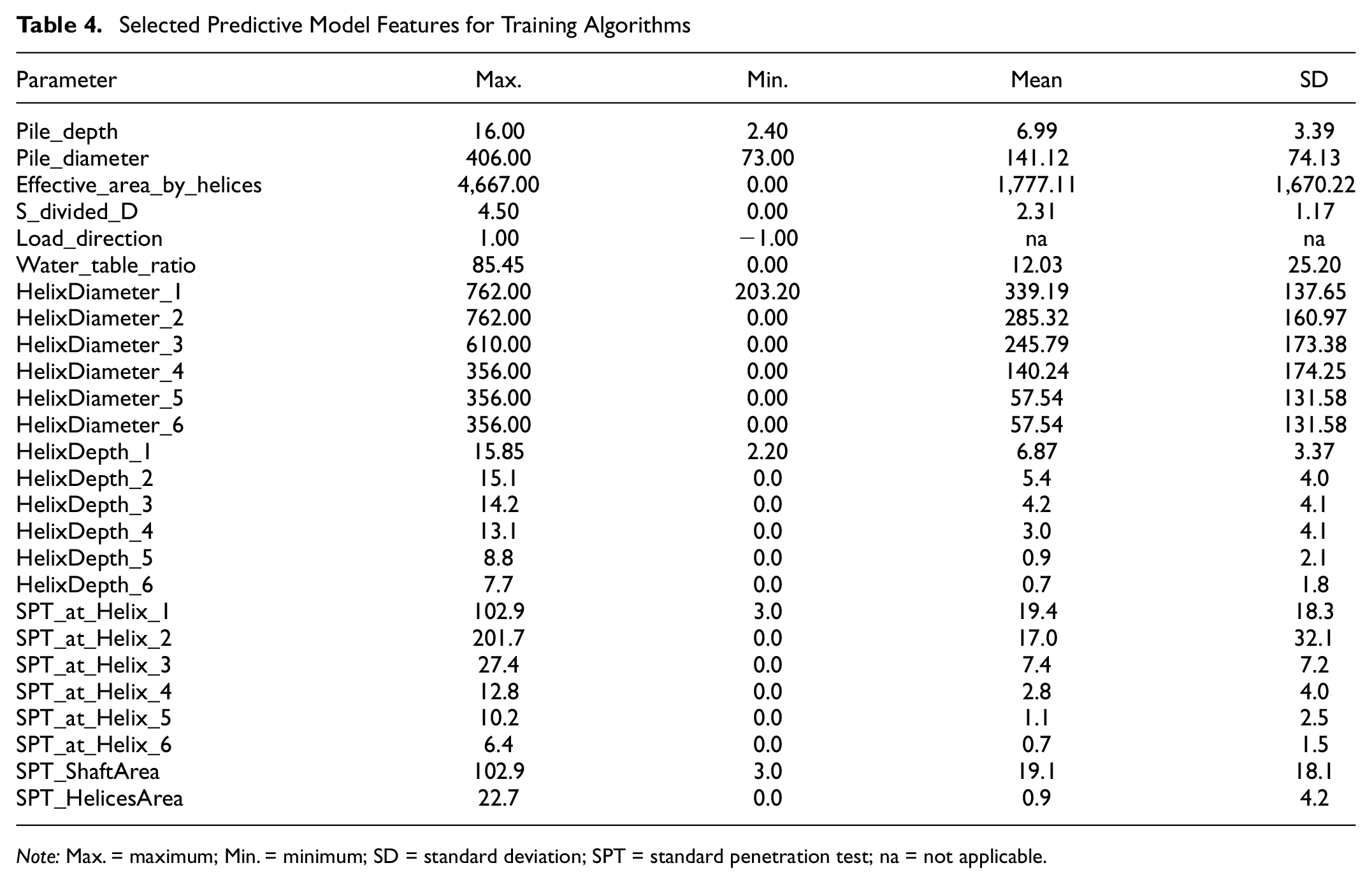
The data preparation for these two categories of features followed the methodology outlined in a study by Rahimi et al. ( 22 ). In their research, Eslami et al. ( 1 ) explored various feature combinations to train MLA for predicting the ultimate load of helical piles and identified the most effective set of features for this purpose. Eslami et al. ( 1 ) investigated how the performance of MLAs is greatly influenced by the correlation between input values, particularly when it comes to helical piles, where design parameters such as embedment depth, shaft diameter, and helix diameter are closely related. It can be difficult to choose the best set of parameters for MLAs because, depending on how they relate to other parameters and how important they are for load-bearing calculations, adding some parameters might either improve or degrade model accuracy. Three different packages (GSP I, GSP II, and GSP III) and every possible combination of fixed characteristics were systematically evaluated to handle this complexity ( 1 ). Pile depth, pile diameter, number of helices, effective helix area, mean helix diameter, maximum and minimum helix diameters, and water table depth (%) were among the permanent features. To capture soil variability across the pile, the floating features in GSP I included the average SPT numbers for areas with and without helices as well as six SPT values for helices. Incorporating the diameters, SPT values, and depths of these crucial sites, GSP II concentrated on the geometry and soil properties at the highest and lowest helix areas. To provide a segmented perspective of soil resistance, GSP III separated the pile embedment depth into five portions and determined the mean SPT values for each region ( 1 ). The features used in this study were selected based on the recommendations provided in their research, as illustrated in Table 4.

Table 4.

Selected Predictive Model Features for Training Algorithms

Parameter	Max.	Min.	Mean	SD
Pile_depth	16.00	2.40	6.99	3.39
Pile_diameter	406.00	73.00	141.12	74.13
Effective_area_by_helices	4,667.00	0.00	1,777.11	1,670.22
S_divided_D	4.50	0.00	2.31	1.17
Load_direction	1.00	−1.00	na	na
Water_table_ratio	85.45	0.00	12.03	25.20
HelixDiameter_1	762.00	203.20	339.19	137.65
HelixDiameter_2	762.00	0.00	285.32	160.97
HelixDiameter_3	610.00	0.00	245.79	173.38
HelixDiameter_4	356.00	0.00	140.24	174.25
HelixDiameter_5	356.00	0.00	57.54	131.58
HelixDiameter_6	356.00	0.00	57.54	131.58
HelixDepth_1	15.85	2.20	6.87	3.37
HelixDepth_2	15.1	0.0	5.4	4.0
HelixDepth_3	14.2	0.0	4.2	4.1
HelixDepth_4	13.1	0.0	3.0	4.1
HelixDepth_5	8.8	0.0	0.9	2.1
HelixDepth_6	7.7	0.0	0.7	1.8
SPT_at_Helix_1	102.9	3.0	19.4	18.3
SPT_at_Helix_2	201.7	0.0	17.0	32.1
SPT_at_Helix_3	27.4	0.0	7.4	7.2
SPT_at_Helix_4	12.8	0.0	2.8	4.0
SPT_at_Helix_5	10.2	0.0	1.1	2.5
SPT_at_Helix_6	6.4	0.0	0.7	1.5
SPT_ShaftArea	102.9	3.0	19.1	18.1
SPT_HelicesArea	22.7	0.0	0.9	4.2

Note: Max. = maximum; Min. = minimum; SD = standard deviation; SPT = standard penetration test; na = not applicable.

The features were selected based on the findings of Eslami et al. ( 1 ), who investigated the influence of various factors on the ultimate load of helical piles. Building on their insights, we identified key features that significantly affect the load-displacement behavior of helical piles. By incorporating factors such as the number of helices, helix diameter, and soil properties, we ensured that our models were equipped with the critical information needed to accurately predict the load-displacement behavior of helical piles.

With regard to Table 4 and Figure 1, the parameters include pile depth, representing the vertical embedment depth of the pile, and pile diameter, which refers to the shaft’s diameter. The effective area by helices indicates the total effective area of all helices contributing to load-bearing capacity, while S-divided-D denotes the ratio of spacing between helices to the shaft diameter, a critical geometric factor. Load direction specifies whether the load is applied axially or laterally, and the water table ratio expresses the relative depth of the water table as a percentage of the pile depth. The helix diameters and their corresponding depths provide detailed geometric information about the pile, influencing soil interaction and load transfer. The SPT values at helix locations represent soil resistance at these depths, while the SPT helix area and SPT shaft area capture the average soil resistance in regions directly influenced by helices and along the shaft, respectively.

Correlation Diagram of Model Features

A heatmap was generated to evaluate the selected features for training MLA. Figure 4 illustrates the pairwise correlation between the features under consideration, providing valuable insights into their interrelationships.

Figure 4.

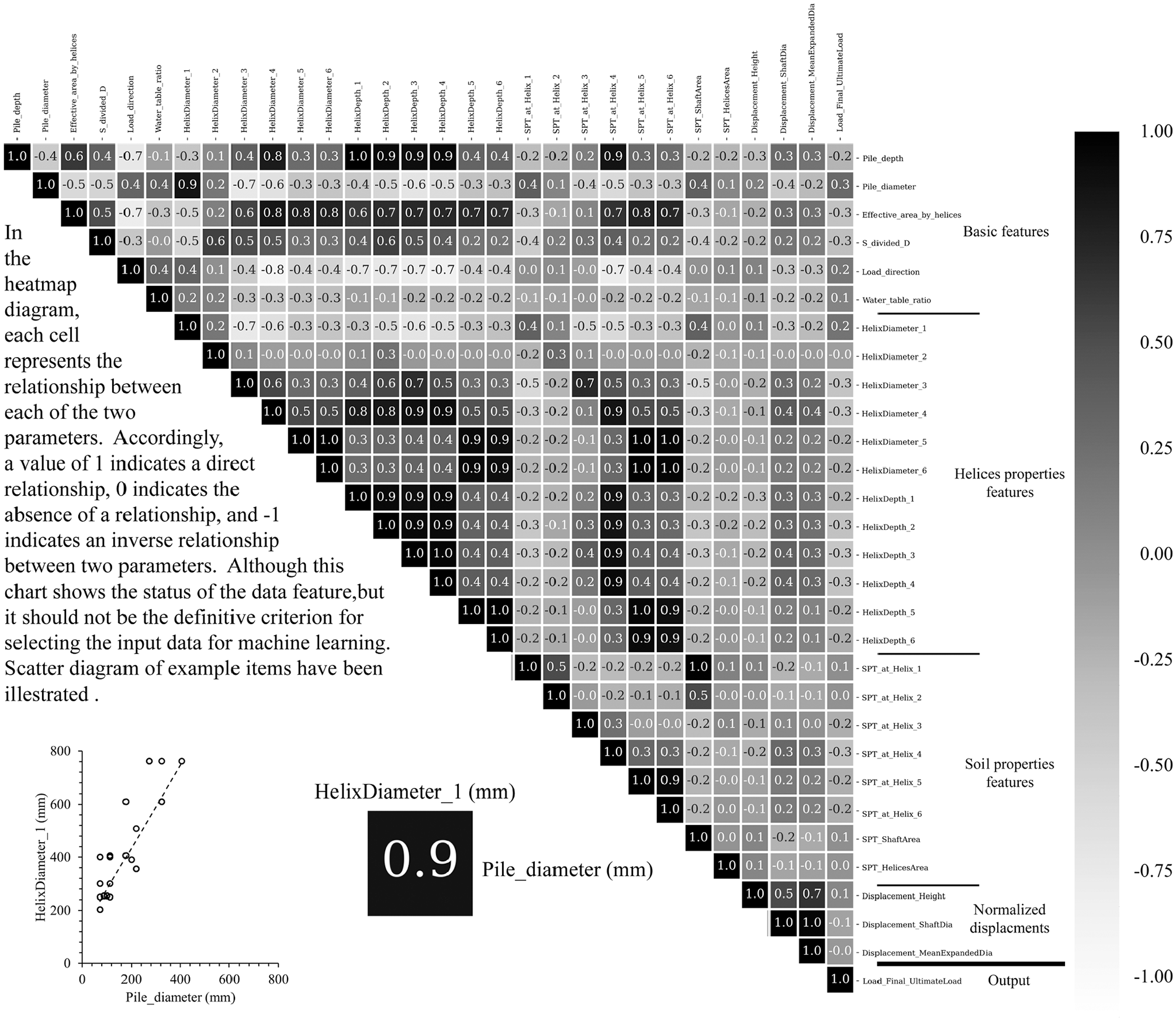
Correlation diagram between predictive model input and output.

A heat map was generated to evaluate the selected features used for training the MLAs. Specifically, the heat map in Figure 4 illustrates the pairwise correlations between the various features under consideration. Each cell in the heat map represents the strength and direction of the correlation between two parameters, with values ranging from −1 to 1. A value of 1 indicates a perfect positive correlation, 0 indicates no correlation, and −1 indicates a perfect negative correlation. This visualization provides critical insights into the interrelationships among the features, which is an important step in feature selection for MLA training. To create the heat map, the correlation coefficients were calculated and the data preprocessing, including normalization of the features, was performed to ensure consistent scaling and comparability between variables. The visualization was generated to ensure clarity and precision.

Methodology

Figure 5 presents the road map of the current study. To predict the load-displacement curve of helical piles based on previous research findings of Eslami et al. ( 1 ), relevant features were extracted from the database for algorithm training. These features included the geometric characteristics of the piles, such as depth, diameter, helix diameter, and helix embedment depth. Additionally, soil properties were incorporated into the analysis by including results from SPT and underground water depth alongside geometric characteristics. SPT was selected as the primary method for analyzing soil parameters and descriptions for several reasons. First, SPT is widely used and recognized in geotechnical engineering, making data more readily available and accessible. Second, established correlations exist between SPT values and key soil parameters, allowing for effective soil description and classification. Third, the data set collected included both SPT and CPT data, and existing correlations allowed for the conversion of CPT data into equivalent SPT values to maintain consistency in analysis. Finally, the data set primarily described soil properties, which presented a broad range of variability that made classification challenging. Therefore, using SPT values was deemed more accurate and practical for analyzing the soil’s influence on the load-displacement behavior of helical piles.

Figure 5.

Flow guideline of selected MLAs in predicting the load-displacement trend of axially loaded helical piles.

Following the methodology outlined in the study by ( 3 ), the load-displacement curve was normalized. For this purpose, by using the ultimate load to normalize the load axis and pile depth, diameter, and mean helix diameter to normalize displacement 3, a normalized curve was obtained (three different classifications in Figure 3).

To validate the trained algorithms, 20% of the piles were randomly selected as unseen data from the data set of 98 piles. The algorithms were trained using the target parameter of load tolerance at each displacement to predict the load-displacement curve of helical piles. Subsequently, the trained algorithms were validated using test pile data. The predictions for the test data were assessed using standard error criteria such as mean absolute error (MAE) and mean squared error (MSE). Finally, the predicted load-displacement curves for the helical piles were compared with measured values based on the algorithm outputs. The steps of this research are briefly shown in Figure 5.

Selected Machine Learning–Based Algorithms (MLA)

In the past, various algorithms have been used by researchers to forecast different parameters in geotechnical engineering ( 1 , 37, 38). In this study, the researchers chose to employ common MLA to focus on determining key features, particularly the normalization methods for load-displacement curves. Using these algorithms not only allows for a more thorough investigation of the factors influencing the accuracy of load-displacement curve prediction but also simplifies the explanation of the calculation methods employed. In this context, five algorithms were examined to predict the load-displacement curve of piles.

Selected Features of MLAs

The correlation among input values significantly influences the performance of various MLAs. In the context of helical piles, where the design factors such as helix diameter, shaft diameter, and embedment depth are intricately interconnected, selecting the right parameters for input into algorithms presents a formidable challenge. The presence of one parameter may either enhance or hinder model accuracy based on its relationships with other parameters and its critical role in load-bearing calculations. To address this complexity, all possible combinations of fixed parameters and the three different packages were systematically evaluated for MLA.

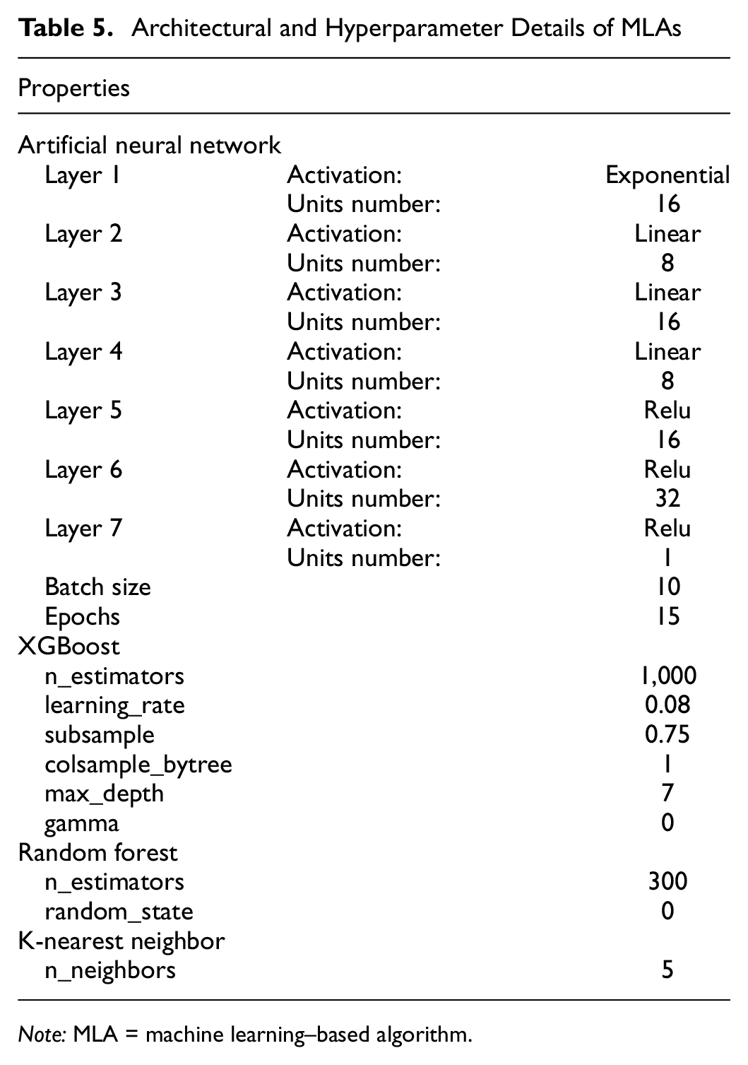
The parameters of the models were selected based on their relevance to the load-displacement behavior of helical piles, as identified in a previous study ( 1 ). These parameters include geometric characteristics (e.g., pile depth, shaft diameter, helix diameter, helix embedment depth) and soil properties derived from SPT results. The selection process aimed to capture the most critical factors influencing load-bearing capacity while minimizing redundancy or noise in the data set. Both parametric and non-parametric models were used to explore the predictive capabilities of MLAs ( 1 , 3 ). Parametric models, such as MLR, assume a predefined functional form and provide interpretable relationships between input features and output. MLR estimates coefficients for each feature to minimize the difference between predicted and actual values, using a simple mathematical framework where the output is a weighted sum of input features plus a bias term ( 1 , 3 ). In contrast, non-parametric models, including KNN, RF, XGB, and ANN, do not rely on predefined assumptions, allowing them to model complex, nonlinear relationships in the data ( 1 , 3 ). KNN predicts the target value based on the values of the KNN in the feature space, capturing local patterns without requiring explicit training. RF, an ensemble learning model, builds multiple decision trees on different data subsets and aggregates their outputs, effectively handling nonlinear relationships and high-dimensional data sets ( 1 , 3 ). XGB, a boosting algorithm, builds trees sequentially, with each tree learning to correct the errors of the previous ones, incorporating regularization techniques to prevent overfitting and ensuring robustness for complex data sets ( 1 , 3 ). ANN, inspired by the human brain, consists of an input layer that accepts the feature set, multiple hidden layers with neurons applying activation functions to capture nonlinear relationships, and an output layer that produces the final prediction ( 1 , 3 ). This dual approach of parametric and non-parametric models enabled a comprehensive analysis of the load-displacement prediction problem by using the strengths of both model types. To address the influence of input correlations on model performance, all possible combinations of fixed parameters and three feature packages (GSP I, GSP II, and GSP III) were systematically evaluated. This evaluation ensured that the models accounted for the intricate relationships between geometric and soil-related features. Hyperparameter optimization for non-parametric models, such as grid search, was employed to fine-tune the models for optimal performance. Table 5 provides the architectural and hyperparameter details of the MLAs used in this study.

Table 5.

Architectural and Hyperparameter Details of MLAs

Properties
Artificial neural network
Layer 1	Activation:	Exponential
	Units number:	16
Layer 2	Activation:	Linear
	Units number:	8
Layer 3	Activation:	Linear
	Units number:	16
Layer 4	Activation:	Linear
	Units number:	8
Layer 5	Activation:	Relu
	Units number:	16
Layer 6	Activation:	Relu
	Units number:	32
Layer 7	Activation:	Relu
	Units number:	1
Batch size		10
Epochs		15
XGBoost
n_estimators		1,000
learning_rate		0.08
subsample		0.75
colsample_bytree		1
max_depth		7
gamma		0
Random forest
n_estimators		300
random_state		0
K-nearest neighbor
n_neighbors		5

Note: MLA = machine learning–based algorithm.

To address the risk of overfitting when working with small sample data sets, several strategies were implemented in this study to ensure model generalization. A k-fold cross-validation technique was used to evaluate performance, which involves dividing the data set into k equally sized subsets (folds). During each iteration, one fold is used as the validation set to test the model’s performance, while the remaining k−1 folds are used for training. The process is repeated k times, allowing every data point to be used exactly once for validation and k−1 times for training. Hyperparameter optimization, through grid search, was applied to tune parameters such as tree depth (RF, XGB), learning rate (XGB), and the number of neurons and layers (ANN), reducing the likelihood of overfitting. Regularization techniques, including L1 and L2 regularization for XGB and dropout layers for ANN, were employed to control model complexity. Early stopping was also used in iterative models such as ANN and XGB by monitoring validation loss and halting training once it ceased to improve.

Evaluation of Model Hyperparameters

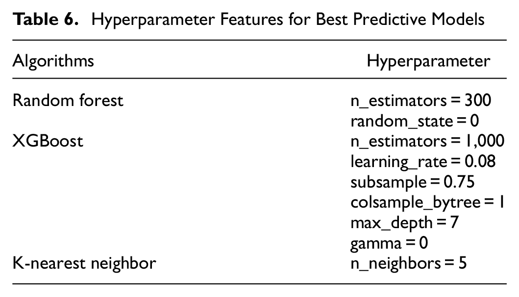
After determining the best combination of input parameters, which was accompanied by initial hyperparameter settings, hyperparameters in each method were manually adjusted using the best combination of input parameters to increase model accuracy and quality. The evaluation for both training and testing employs identical hyperparameter configurations. Table 6 displays the hyperparameter combination derived from the final predictive model.

Table 6.

Hyperparameter Features for Best Predictive Models

Algorithms	Hyperparameter
Random forest	n_estimators = 300
	random_state = 0
XGBoost	n_estimators = 1,000
	learning_rate = 0.08
	subsample = 0.75
	colsample_bytree = 1
	max_depth = 7
	gamma = 0
K-nearest neighbor	n_neighbors = 5

Predictive Model Performance Metrics

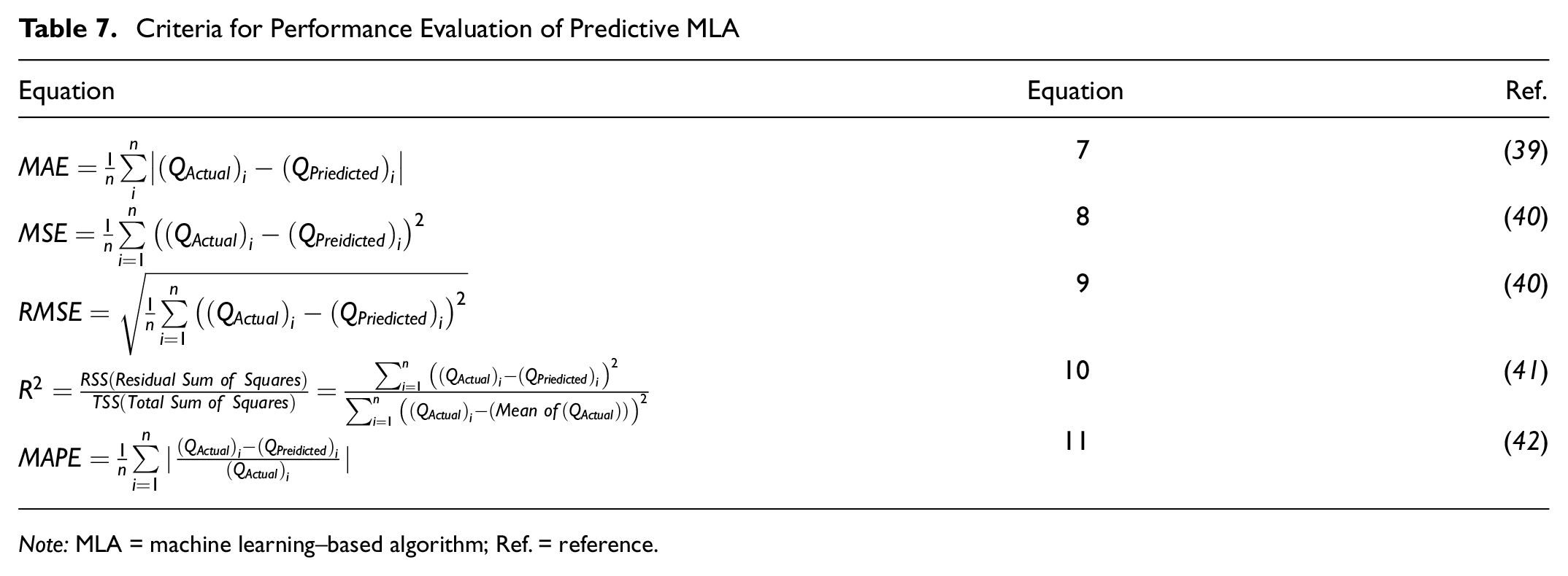
To evaluate the ML models, five metrics (Equations 7–11), including mean absolute error (MAE), mean squared error (MSE), root mean squared error (RMSE), R², and mean absolute percentage error (MAPE), have been used (Table 7). In most previous studies, researchers reported the accuracy of their models based on the first four metrics, which are directly related to the magnitude of the predicted feature. However, given the variability of load-bearing values in different data sets, it is not possible to compare the accuracy of different models solely based on these metrics. Moreover, using R² as a metric can lead to false results because the use of the average of actual values in the denominator of the fraction increases with the increase in the number of data and finally causes a false increase in the R² values. Therefore, R² is not a suitable metric for comparing different studies with different data distributions. In this study, in addition to the first four metrics, MAPE was used to provide a more accurate assessment of the MLA ( 14 ).

Table 7.

Criteria for Performance Evaluation of Predictive MLA

Equation	Equation	Ref.
$MAE = \frac{1}{n} \sum_{i}^{n} \| {(Q_{Actual})}_{i} - {(Q_{Priedicted})}_{i} \|$	7	( 39 )
$MSE = \frac{1}{n} \sum_{i = 1}^{n} {({(Q_{Actual})}_{i} - {(Q_{Preidicted})}_{i})}^{2}$	8	( 40 )
$RMSE = \sqrt{\frac{1}{n} \sum_{i = 1}^{n} {({(Q_{Actual})}_{i} - {(Q_{Priedicted})}_{i})}^{2}}$	9	( 40 )
$R^{2} = \frac{RSS (Residual Sum of Squares)}{TSS (Total Sum of Squares)} = \frac{\sum_{i = 1}^{n} {({(Q_{Actual})}_{i} - {(Q_{Priedicted})}_{i})}^{2}}{\sum_{i = 1}^{n} {({(Q_{Actual})}_{i} - (Mean of (Q_{Actual})))}^{2}}$	10	( 41 )
$MAPE = \frac{1}{n} \sum_{i = 1}^{n} \| \frac{{(Q_{Actual})}_{i} - {(Q_{Preidicted})}_{i}}{{(Q_{Actual})}_{i}} \|$	11	( 42 )

Note: MLA = machine learning–based algorithm; Ref. = reference.

Predictive Model Results and Validation

MLA Evaluative Metrics

The findings of this research can be analyzed through two distinct lenses. The first perspective involves evaluating the impact of altering the normalization technique for load-displacement curves on the predictive performance of each algorithm. The second perspective entails assessing the prediction accuracy of various MLAs across different data sets. Subsequently, we will delve into the results derived from these dual viewpoints.

The spider diagrams in Figure 6 display the metrics obtained from predicting test data using five MLAs across three data sets. The performance of the MLR and ANN algorithms appears to be relatively weaker compared with the others. On closer inspection of individual graphs, the impact of normalizing load-displacement curve data on the accuracy of the ANN method becomes evident. Among the metrics used, MAPE stands out as the sole measure enabling comparisons across data sets of varying scales. Analysis of Figure 6 suggests that Data set 1 exhibits lower prediction accuracy than the other two data sets. Based on this, we can draw conclusions by normalizing load-displacement data based on pile diameter and mean helices diameter, which yields superior results compared with normalization using pile depth.

Figure 6.

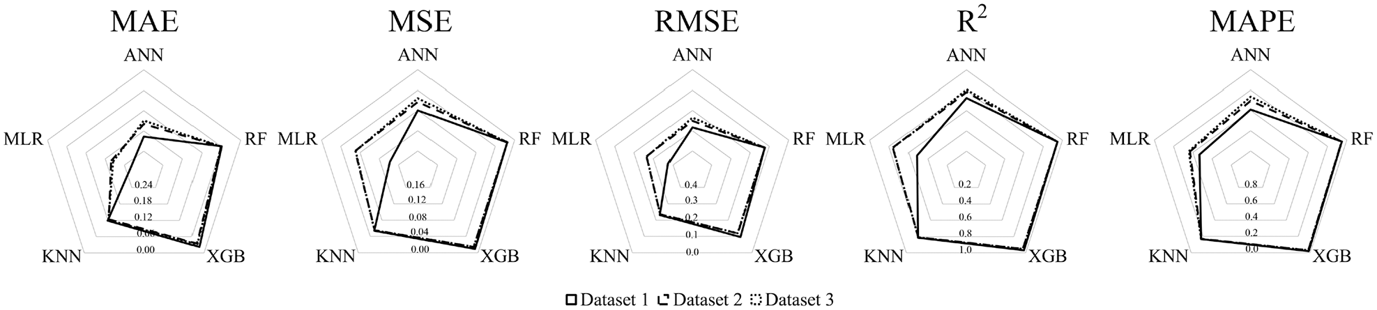
Results of predictive model performance metrics.

Regression Error Characteristic (REC)

To further analyze the performance of the algorithms in the prediction of test data, the REC charts were used; the results are illustrated in Figure 7. Each graph is accompanied by a table detailing the area over the REC curve (AOC) and the area under the REC curve (AUC). Given that reducing the area over the REC curve increases the prediction accuracy, the three methods, XGB, RF, and KNN, have shown the best results, and the results observed in the previous figures have been confirmed. Additionally, the impact of data normalization on the ANN algorithm is clearly depicted in these graphs.

Figure 7.

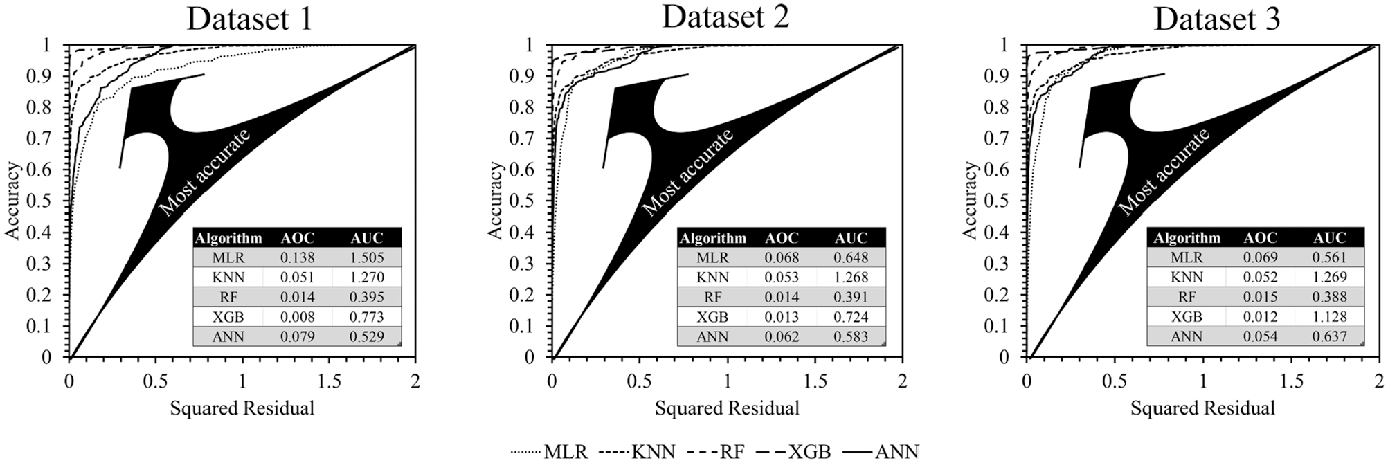
Regression error characteristic (REC) for best feature combination in all MLA.

Performance of Selected MLAs

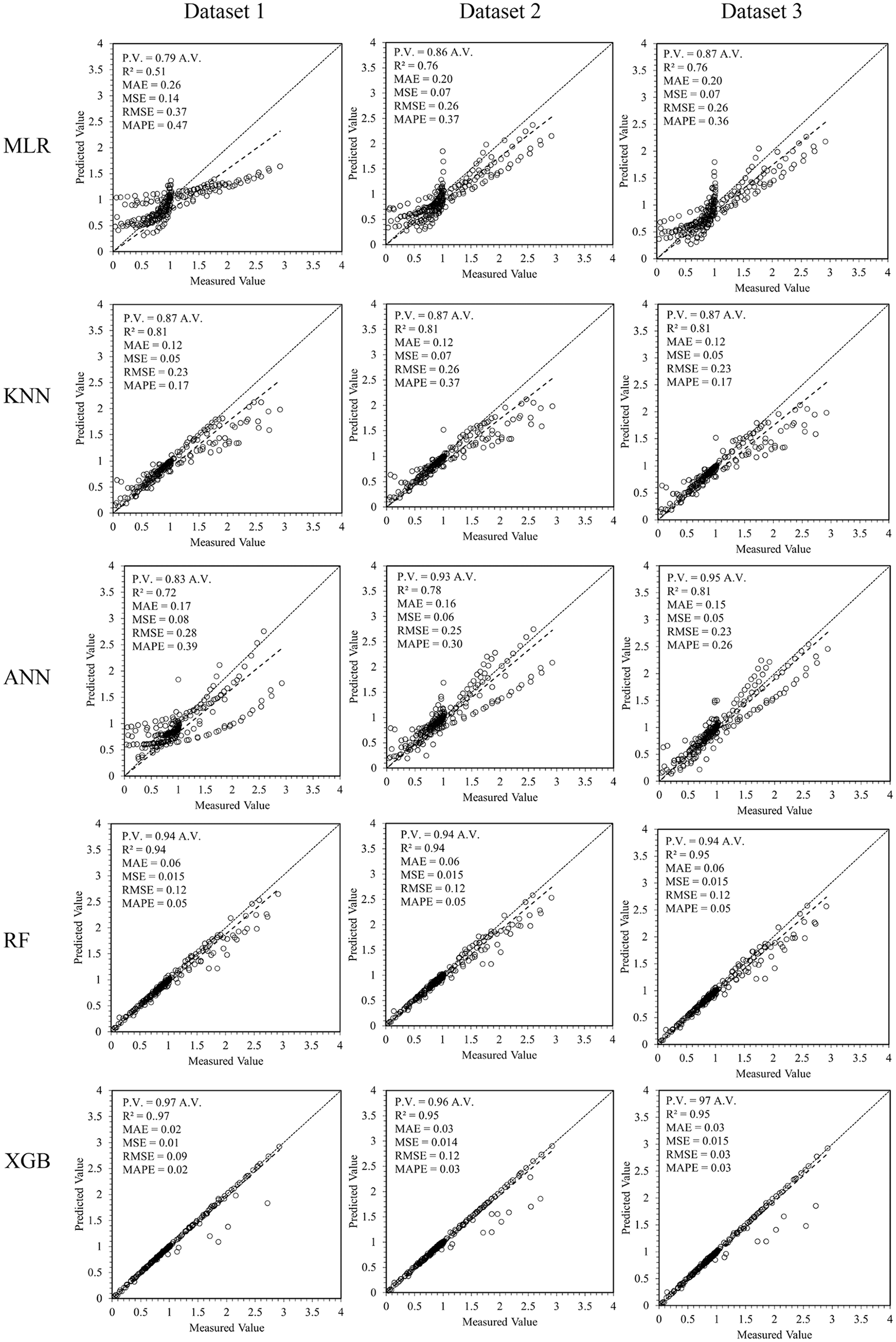
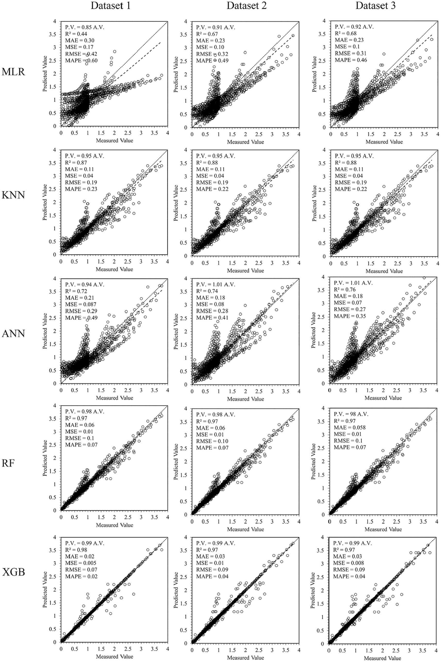
To illustrate the comparison between measured and predicted values across all three data sets using the five learning algorithms, Figures 8 and 9 were generated. In each diagram, the horizontal axis represents the measured values, while the vertical axis displays the predicted values. As the data points converge toward the dotted line, indicative of perfect alignment, the predictive accuracy improves.

Figure 8.

Performance of predicted MLA on testing data.

Figure 9.

Performance of predicted MLA on training data.

Analysis of Figures 8 and 9, shows that XGB, RF, and KNN consistently demonstrate superior prediction quality across the data sets. Additionally, a marginal enhancement in accuracy is observed when transitioning from Data set 1 to Data set 3 within each algorithm. Notably, XGB stands out as the most effective algorithm, particularly when applied to Data set 3.

Predicted Load-Displacement Curved Trending

Figure 10 displays the predicted load-displacement curves for three sample piles subjected to algorithm testing. It is evident from the graph that the ANN and MLR algorithms exhibit higher discrepancies from the measured values when compared with other algorithms used in the study.

Figure 10.

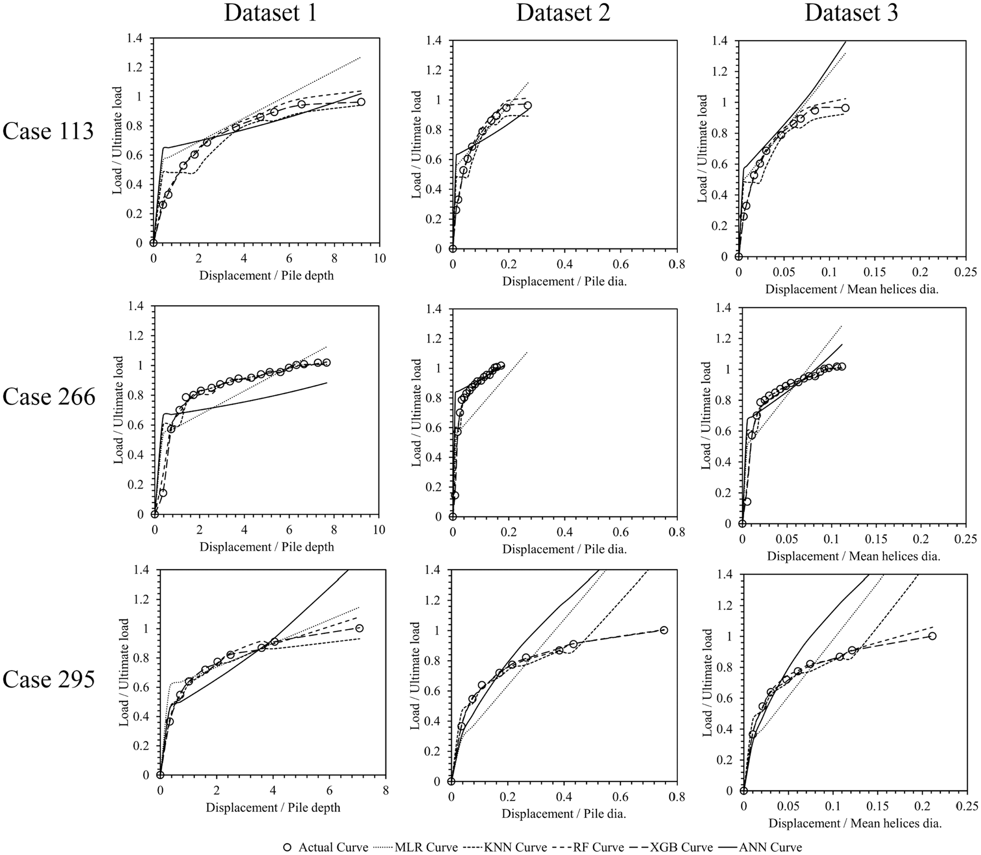
Helical piles predicted load-displacement trend via MLA.

Discussion of the Developed Predicted Models: Sensitivity Analysis and Limitations

Data Set’s Influence

In analyzing the results derived from the predicate test data, it is evident that normalizing displacement in the load-displacement curve can enhance the correlation between the curve’s shape and geometric parameters. This normalization process can significantly improve prediction accuracy in algorithms using decision trees or nearest-neighbor methods. Selecting the appropriate parameter for normalizing the load-displacement curve is crucial for enhancing prediction accuracy, warranting further exploration in future research endeavors.

Furthermore, the examination of three displacement normalization parameters (pile depth, pile diameter, mean helices diameter) on the load-displacement curve revealed that using the mean helices diameter for normalization, as opposed to pile depth, resulted in a higher number of accurately predicted values. The significance of this finding underscores the need for meticulous consideration when choosing normalization parameters. Additionally, the method of determining the ultimate load can affect forecast accuracy, prompting a call for more in-depth investigations into this aspect.

Features

Based on previous research conducted by Eslami et al. ( 1 ), the geometric and soil characteristics selected as features for algorithm training have proven to yield favorable results in prediction accuracy. However, future studies could benefit from exploring the inclusion of data obtained from CPT to further enhance the predictive capabilities of the algorithms.

Sensitivity Analysis

The sensitivity analysis, reported by Davar et al. ( 43 ), of input parameters based on the predictive models results involves examining how variations in these parameters affect the outcomes predicted by the models. Moreover, it was observed that among the selected predictive models, XGB, RF, and KNN demonstrated promising performance, showing good results with input parameters such as pile geometry, helix geometry, and soil characteristics surrounding the helix (Figure 11). This process helps in understanding the influence and significance of different inputs on the model’s predictions, thereby providing insights into the robustness and reliability of the predictive models.

Figure 11.

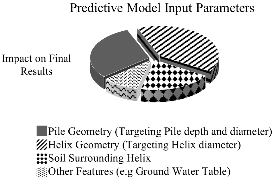
Sensitivity analysis of input parameters based on the predictive model results.

Errors

According to the error percentage analysis of the predicted values in comparison to the measured values, it was observed that the errors in small displacements were predominantly positive, indicating an overall tendency for overestimation. The significant errors observed in these regions are attributed to the relatively low measured loads present at the initial stages of curve movement.

To evaluate the accuracy of the algorithms in predicting load-displacement curves, Figure 12 illustrates the errors between predicted and measured load values. Negative values on the graphs indicate an underestimation of loads by the algorithms. Analysis reveals that the MLR and KNN methods generally overestimate loads, while the ANN algorithm initially overestimates but later underestimates. The RF and XGB algorithms exhibit a balance of negative and positive errors. Notably, as data sets progress from 1 to 3, all algorithms show a trend of decreasing negative errors and increasing positive errors.

Figure 12.

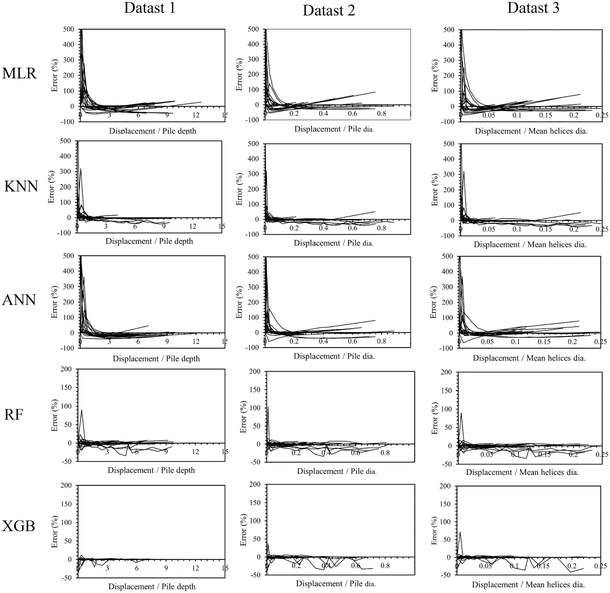
Model performance error variations in each data set for MLAs.

A notable observation from the analysis of Figure 12 is the significant error values present at the initial stages of the load-displacement curve of the pile. This discrepancy arises from the low measured load applied during small displacements, leading the error percentage to significant values. In summary, based on this observation, it is evident that most algorithms exhibit elevated error percentage values at the initial segment of the graph.

The errors between predicted and measured values, as observed in Figure 12, stem from multiple sources, including model-related, data-related, and feature-related factors. Model-related errors arise from the limitations of certain algorithms, such as MLR and KNN, which struggle to capture complex nonlinear relationships, while occasional overfitting or underfitting can affect models such as ANN, RF, and XGB. Data-related errors may be caused by noise, measurement inconsistencies, or the limited size of the data set, which can restrict the generalizability of more complex models. Feature-related errors stem from variability in input features, such as soil properties and geometric parameters, and the choice of normalization parameters, with Data set 3 (normalized by mean helix diameter) consistently showing better performance. To reduce these errors, strategies such as improving data quality and quantity, refining feature selection, optimizing model hyperparameters, applying effective normalization techniques, and using ensemble or hybrid models can be employed.

Factors Influencing Accuracy Differences Across Algorithms

An important aspect to consider in this review is the notable disparities in the prediction results obtained from XGB, RF, and KNN algorithms compared with MLR and ANN algorithms ( 44 ). The lack of accuracy in the predictions made by the MLR algorithm can be attributed to its calculation method. As demonstrated in the heatmap analysis, the features associated with helical piles, particularly when sourced from diverse sites, may not exhibit a clear linear relationship, thereby affecting the predictive accuracy of this algorithm. Similarly, the poor performance of the ANN algorithm can be attributed to its requirement for a larger data set. Given the diverse range of test sites used in this study, it is plausible that employing the ANN algorithm on a smaller number of test sites with a greater number of piles could potentially enhance its predictive accuracy.

Practical Applicability and Limitations of MLAs in Engineering Design and Construction

The MLAs’ direct application to design and construction guidance requires careful consideration of both their potential and limitations. Compared with available empirical methods and numerical simulations, these MLAs provide a data-driven alternative that can capture complex relationships between input parameters and load-displacement behavior, offering high accuracy and computational efficiency. However, they rely heavily on the quality and representativeness of the training data set. For practical engineering decision making, these models must be validated against diverse site-specific conditions to ensure reliability across various scenarios. Additionally, while MLAs excel in prediction, they lack the interpretability of available empirical methods and numerical simulations and do not inherently provide insights into the underlying physics of soil–pile interaction. As such, they are best used as a complementary tool alongside available empirical methods and numerical simulations to enhance efficiency and provide initial evaluations. To bridge the gap between model predictions and practical usability, a deliverable product from this study will be a user-interface software package. This tool will allow engineers to upload their site-specific data, input new data sets, select the desired predictive model, and obtain the predicted load-displacement trend. This software will make the models more accessible and operable for practitioners, offering a streamlined workflow for integrating ML predictions into design and construction processes.

Conclusions

This research study focused on predicting the load-displacement curve of helical piles, using data from the available complied database. Specifically, 98 helical piles were selected from this database, and their load-displacement curves were normalized using three distinct methods, resulting in three separate data sets. A comprehensive approach was adopted to forecast these curves, employing multiple algorithms, including MLR, KNN, ANN, RF, and XGB. Additionally, to evaluate the efficacy of these algorithms, 20 piles (20% of the data sets) were randomly allocated as unseen data for testing. The test set was selected through a random sampling process to ensure that the testing data remained independent of the training data. This random allocation helps to reduce bias and ensures that the test set is unseen during model training. To maintain representativeness, the random sampling was conducted in a manner that reflects the diversity and variability of the entire data set, including variations in soil properties, pile geometry, and other critical input features. By integrating various MLA and leveraging a sizable data set, this research contributes to advancing the predictive capabilities in the field of helical pile analysis and design. Derived from the findings of this investigation, the subsequent conclusions can be inferred:

○ MLAs offer a viable means to predict the load-displacement curve of helical piles, potentially reducing testing expenses and time requirements.

○ The normalization techniques applied to load-displacement curves significantly influenced the predictive accuracy of the algorithms. Notably, using the mean diameter of helices relative to pile depth to normalize the displacement axis resulted in increased positive errors. This underscores the importance of the chosen parameter for curve normalization and necessitates deeper exploration in subsequent research endeavors.

○ The optimal MLA performance results were achieved with the XGB, RF, and KNN algorithms. However, the performance of these algorithms is contingent on the characteristics of the training sites, potentially leading to decreased accuracy when forecasting piles from different locations.

○ The ANN method demonstrated subpar performance. Augmenting the data set with more piles and narrowing the scope of investigated sites could enhance prediction accuracy using this algorithm.

○ Across all data sets, XGB and RF consistently exhibit the lowest prediction errors, demonstrating their ability to model complex nonlinear relationships. ANN performs moderately well but shows higher errors compared with XGB and RF, while KNN and MLR display higher variability and larger errors, indicating lower reliability for predicting load-displacement behavior. Errors across all models generally decrease as normalized displacement values increase, with smaller displacements showing higher complexity and variability. Data set 3, normalized by mean helix diameter, results in improved performance for all models, particularly for XGB and RF, suggesting that this normalization better captures the load-displacement trends.

○ Pile geometry and helix geometry account for a significant portion of the model’s sensitivity, emphasizing their critical role in influencing the load-displacement behavior of helical piles. Soil properties surrounding the helix also play a substantial role, reflecting the importance of capturing soil-structure interactions accurately.

○ Considering the predicted and actual load-displacement curves for three test cases across three data sets, XGB and RF consistently deliver the most accurate predictions, closely aligning with the actual curves, while ANN shows moderate performance but with noticeable deviations at higher displacements. In contrast, KNN and MLR struggle to capture the shape of the curves, particularly at the initial and later stages of displacement. Data set 3, normalized by mean helix diameter, consistently provides better results across all models, indicating that this normalization captures the relationship between load and displacement more effectively.

○ Comparing predicted values to measured values across three data sets of five MLAs for training data sets, XGB and RF consistently deliver the best performance, achieving R² values close to 0.97 and exhibiting minimal errors across all data sets. ANN and KNN demonstrate moderate accuracy, with slightly higher error values, while MLR shows the weakest performance.

○ For testing data sets, among the models, XGB consistently demonstrates the best performance across all data sets, with high R² values (0.95–0.97) and minimal errors (MAE, MSE, RMSE, and MAPE). RF also performs exceptionally well, showing R² values around 0.94 and similarly low error metrics. ANN and KNN exhibit moderate performance, with ANN showing higher accuracy in Data sets 2 and 3. MLR consistently underperforms compared with the other models, with lower R² values (0.51–0.76) and higher error metrics, reflecting its limited capability to handle complex relationships.

○ Considering REC curves for the best feature combination in five MLAs across three data sets, XGB consistently outperforms the other models, achieving the highest AUC values (0.773, 0.724, and 0.728) and the lowest AOC values across all data sets, followed closely by RF. ANN and KNN demonstrate moderate performance, while MLR performs the worst, with the lowest AUC values and highest AOC values, reflecting its limited ability to handle complex relationships.

Footnotes

Acknowledgements

The authors would like to thank graduate research assistants, engineers, and others, those who helped make this research possible.

Author Contributions

The authors confirm contribution to the paper as follows: study conception and design: Abolfazl Eslami, Masoud Nobahar; data collection: Masoud Nobahar, Amirhossein Rahimi; analysis and interpretation of results: Masoud Nobahar, Amirhossein Rahimi; draft manuscript preparation: Masoud Nobahar. All authors reviewed the results and approved the final version of the manuscript.

Declaration of Conflicting Interests

The author(s) declared no potential conflicts of interest with respect to the research, authorship, and/or publication of this article.

Funding

The author(s) received no financial support for the research, authorship, and/or publication of this article.

ORCID iDs

Masoud Nobahar

Amirhossein Rahimi

Data Accessibility Statement

The data that supports the findings of this study are available from the corresponding author, on request.

References

Eslami

Rahimi

Nobahar

Ultimate Load Bearing of Helical Piles Prediction and Evaluation Using Machine Learning-Based Algorithms. An International Journal of Geomechanics and Geoengineering, Vol. 20, 2024, pp. 1–26. https://doi.org/10.1080/17486025.2024.2438077.

Shojaei

Eslami

Ganjian

Self-Expanded Piles: A New Approach to Unconventional Piles Development. Marine Georesources & Geotechnology, Vol. 39, No. 1, 2021, pp. 115–128.

Abu-Farsakh

M. Y.

Shoaib

M. M.

Machine Learning Models to Evaluate the Load Settlement Trend of Piles from Cone Penetration Test Data. Geotechnical and Geological Engineering, Vol. 42, No. 5, 2024, pp. 3433–3449. https://doi.org/10.1007/s10706-023-02737-6.

Perko

H. A.

Helical Piles: A Practical Guide to Design and Installation. John Wiley & Sons, Hoboken, NJ, 2009.

CFEM. Canadian Foundation Engineering Manual, 4th ed. Bi-Tech Publisher Ltd, Vancouver, Canada, 2006.

IBC (International Building Code). Acceptance Criteria for Helical Foundation Systems and Devices (AC358). International Code Council Evaluation Service, Brea, CA, 2009.

Nobahar

Khan

M. S.

Prediction of Matric Suction of Highway Slopes Using Autoregression Artificial Neural Network (ANN) Model. Geo-Extreme, Vol. 2021, 2021, pp. 40–50.

Khan

M. S.

Ivoke

Nobahar

Amini

Artificial Neural Network (ANN) Based Soil Temperature Model of Highly Plastic clay. Geomechanics and Geoengineering, Vol. 17, No. 4, 2022, pp. 1230–1246.

Ismail

Jeng

D.-S.

Modelling Load–Settlement Behaviour of Piles Using High-Order Neural Network (HON-PILE Model). Engineering Applications of Artificial Intelligence, Vol. 24, No. 5, 2011, pp. 813–821.

10.

Shuman

N. M.

Khan

M. S.

Amini

Efficient Machine Learning Model for Settlement Prediction of Large Diameter Helical Pile in c—Φ Soil. AI in Civil Engineering, Vol. 3, No. 1, 2024, p. 10.

11.

Galton

Regression Towards Mediocrity in Hereditary Stature. The Journal of the Anthropological Institute of Great Britain and Ireland, Vol. 15, 1886, pp. 246–263. https://doi.org/10.2307/2841583.

12.

Fix

Hodges

J. L.

Discriminatory Analysis. Nonparametric Discrimination: Consistency Properties. International Statistical Review / Revue Internationale de Statistique, Vol. 57, No. 3, 1989, pp. 238–247. https://doi.org/10.2307/1403797.

13.

Breiman

Random Forests. Machine Learning, Vol. 45, No. 1, 2001, pp. 5–32. https://doi.org/10.1023/A:1010933404324.

14.

Chen

Guestrin

XGBoost: A Scalable Tree Boosting System. Proceedings of the ACM SIGKDD International Conference on Knowledge Discovery and Data Mining. 2016. https://doi.org/10.1145/2939672.2939785.

15.

Wang

Moayedi

Nguyen

Foong

L. K.

Rashid

A. S. A.

Feasibility of a Novel Predictive Technique Based on Artificial Neural Network Optimized With Particle Swarm Optimization Estimating Pullout Bearing Capacity of Helical Piles. Engineering with Computers, Vol. 36, 2020, pp. 1315–1324.

16.

Wang

Chen

Hao

Tian

Efficient Machine Learning Models for the Uplift Behavior of Helical Anchors in Dense Sand for Wind Energy Harvesting. Applied Sciences, Vol. 12, No. 20, 2022, p. 10397.

17.

Ismail

Jeng

D.-S.

Zhang

L. L.

An Optimised Product-Unit Neural Network With a Novel PSO–BP Hybrid Training Algorithm: Applications to Load–Deformation Analysis of Axially Loaded Piles. Engineering Applications of Artificial Intelligence, Vol. 26, No. 10, 2013, pp. 2305–2314.

18.

Nejad

F. P.

Jaksa

M. B.

Kakhi

McCabe

B. A.

Prediction of Pile Settlement Using Artificial Neural Networks Based on Standard Penetration Test Data. Computers and Geotechnics, Vol. 36, No. 7, 2009, pp. 1125–1133.

19.

Shahin

M. A.

Load–Settlement Modeling of Axially Loaded Drilled Shafts Using CPT-Based Recurrent Neural Networks. International Journal of Geomechanics, Vol. 14, No. 6, 2014, p. 06014012.

20.

Nejad

F. P.

Jaksa

M. B.

Load Settlement Trend Modeling of Single Piles Using Artificial Neural Networks and CPT Data. Computers and Geotechnics, Vol. 89, 2017, pp. 9–21.

21.

Moayedi

Hayati

Applicability of a CPT-Based Neural Network Solution in Predicting Load Settlement Responses of Bored Pile. International Journal of Geomechanics, Vol. 18, No. 6, 2018, p. 06018009.

22.

Rahimi

Load Displacement Analysis of Different Expanded Pile for Using in Marine Structures. Amirkabir University of Technology (Tehran Polytechnic), 2022.

23.

Sakr

Performance of Helical Piles in Oil Sand. Canadian Geotechnical Journal, Vol. 46, No. 9, 2009, pp. 1046–1061. https://doi.org/10.1139/T09-044.

24.

Elsherbiny

El Naggar

M. H.

The Performance of Helical Pile Groups under Compressive Loads: A Numerical Investigation. 18th International Conference on Soil Mechanics and Geotechnical Engineering: Challenges and Innovations in Geotechnics, ICSMGE 2013, Vol. 4, No. 3, 2013, pp. 2723–2726.

25.

Sakr. Comparison between High Strain Dynamic and Static Load Tests of Helical Piles in Cohesive Soils. Soil Dynamics and Earthquake Engineering, Vol. 54, 2013, pp. 20–30. https://doi.org/10.1016/j.soildyn.2013.07.010.

26.

Fahmy

El Naggar

M. Hesham

. Axial Performance of Helical Tapered Piles in Sand.” Geotechnical and Geological Engineering, Vol. 35, No. 4, 2017, pp. 1549–1576. https://doi.org/10.1007/s10706-017-0192-1.

27.

Beim

Luna

S. C.

Results of Dynamic and Static Load Tests on Helical Piles in the Varved clay of Massachusetts. DFI Journal - The Journal of the Deep Foundations Institute, Vol. 6, No. 1, 2012, pp. 58–67. https://doi.org/10.1179/dfi.2012.005.

28.

Lee

Kim

H.-N.

Choi

Effect of Configuration of Shaft and Helix Plate on Bearing Capacity of Moderate-Size Helical Pile : I. Test-Bed Construction and Field Loading Test. Journal of the Korean Geosynthetics Society, Vol. 13, No. 2, 2014, pp. 31–39. https://doi.org/10.12814/JKGSS.2014.13.2.031.

29.

Zhang

D. J. Y.

Predicting Capacity of Helical Screw Piles in Alberta Soils. University of Alberta, 1999, pp. 1–304.

30.

Dos Santos Filho

J. M. S. M.

Tsuha

C. de H. C.

Uplift Performance of Helical Piles with Cement Injection in Residual Soils. Canadian Geotechnical Journal, Vol. 57, No. 9, 2019, pp. 1335–1355. https://doi.org/10.1139/CGJ-2019-0317.

31.

Tappenden

K. M.

Predicting the Axial Capacity of Screw Piles Installed in Western Canadian Soils. University of Alberta, 2007, pp. 1–193. https://era.library.ualberta.ca/files/bv73c235m/4008200.pdf.

32.

Skempton

A. W.

Standard Penetration Test Procedures and the Effects in Sands of Overburden Pressure, Relative Density, Particle Size, Ageing and Overconsolidation. Géotechnique, Vol. 36, No. 3, 1986, pp. 425–447. https://doi.org/10.1680/geot.1986.36.3.425.

33.

Bolton Seed

Tokimatsu

Harder

L. F.

Chung

R. M.

Influence of SPT Procedures in Soil Liquefaction Resistance Evaluations. Journal of Geotechnical Engineering, Vol. 111, No. 12, 1985, pp. 1425–1445. https://doi.org/10.1061/(ASCE)0733-9410(1985)111:12(1425).

34.

Lunne

Robertson

P. K.

Powell

J. J. M.

Cone Penetration Testing in Geotechnical Practice. Blackie Academic and Professional, London, 1997.

35.

Campanella

R. G.

Robertson

P. K.

Gillespie

Grieg

Use of Piezometer Cone Data. Proceedings of American Society of Civil Engineering, ASCE, In-Situ 86 Specialty Conference, 1986b, p. 1263e1280. Publication GSP No. 6.

36.

Eslami

Fellenius

B. H.

CPT and CPTu Data for Soil Profile Interpretation: Review of Methods and a Proposed New Approach. Iran Journal of Science and Technology, Transection B, Vol. 28, No. B1, 2004, p. 69e86.

37.

Thai

P. B.

Nguyen

D. D.

Bui Thi

Q.-A.

Nguyen

M. D.

T. T.

Prakash

Estimation of Ultimate Bearing Capacity of Bored Piles Using Machine Learning Models. Vietnam Journal of Earth Sciences, Vol. 44, No. 4, 2022, 470–480. https://doi.org/10.15625/2615-9783/17177.

38.

Ozturk

Kodsy

Iskander

Forecasting the Capacity of Open-Ended Pipe Piles Using Machine Learning. Infrastructures, Vol. 8, No. 1, 2023, p. 12. https://doi.org/10.3390/infrastructures8010012.

39.

Willmott

C. J.

On the Validation of Models. Physical Geography, Vol. 2, No. 2, 1981, pp. 184–194. https://doi.org/10.1080/02723646.1981.10642213.

40.

Geurts

Box

G. E. P.

Jenkins

G. M.

Time Series Analysis: Forecasting and Control. Journal of Marketing Research, Vol. 14, No. 2, 1977, p. 269. https://doi.org/10.2307/3150485.

41.

Pearson

Mathematical Contributions to the Theory of Evolution. On a Form of Spurious Correlation Which May Arise When Indices Are Used in the Measurement of Organs. Proceedings of the Royal Society of London, Vol. 60, No. 359–367, 1897, pp. 489–498. https://doi.org/10.1098/rspl.1896.0076.

42.

Fildes

Scott Armstrong

Long-Range Forecasting: From Crystal Ball to Computer. The Journal of the Operational Research Society, Vol. 30, No. 7, 1979, pp. 673–674. https://doi.org/10.2307/3009390.

43.

Davar

Nobahar

Khan

M. S.

Amini

The Development of PSO-ANN and BOA-ANN Models for Predicting Matric Suction in Expansive clay Soil. Mathematics, Vol. 10, No. 16, 2022, p. 2825.

44.

Masoud

Han

Eslami

Khan

Amini

Stability Prediction of Highway Slope on Highly Plastic clay Using Particle Swarm Optimization (PSO)-Based Neural Network. Geo-Congress, 2024, pp. 264–274.

Predicting and Evaluating Load-Displacement Trends of Helical Piles Using Machine Learning–Based Algorithms

Abstract

Keywords

Data Set

Description

Preparation

Calculate Ultimate Load

Load-Displacement Curves Normalization and Model Framework

Soil Properties

Correlation Diagram of Model Features

Methodology

Selected Machine Learning–Based Algorithms (MLA)

Selected Features of MLAs

Evaluation of Model Hyperparameters

Predictive Model Performance Metrics

Predictive Model Results and Validation

MLA Evaluative Metrics

Regression Error Characteristic (REC)

Performance of Selected MLAs

Predicted Load-Displacement Curved Trending

Discussion of the Developed Predicted Models: Sensitivity Analysis and Limitations

Data Set’s Influence

Features

Sensitivity Analysis

Errors

Factors Influencing Accuracy Differences Across Algorithms

Practical Applicability and Limitations of MLAs in Engineering Design and Construction

Conclusions

Footnotes

Acknowledgements

Author Contributions

Declaration of Conflicting Interests

Funding

ORCID iDs

Data Accessibility Statement

References