
Abstract
Surrogate safety measures (SSM) have been used extensively in traffic safety studies for crash risk estimation. Most SSM-based studies employing extreme value theory (EVT) use the peak over threshold (POT) approach to detect anomalies or extreme events during safety-critical situations. This study investigated the efficacy of unsupervised machine learning (ML)-based anomaly detection methods as an extreme event sampling approach compared with the conventional POT sampling approach by developing bivariate EVT models for rear-end crash risk estimation on a freeway segment. Three widely used SSMs, namely time-to-collision (TTC), modified time-to-collision (MTTC), and deceleration rate to avoid crash (DRAC), were considered for the bivariate EVT modeling. Video data were collected from the selected segment of the I-40 expressway in Memphis, Tennessee. Among three SSMs, the combination of MTTC and DRAC bivariate EVT models provided the most accurate crash risk estimation (within the 99% confidence interval of the observed crashes), applying the traditional POT sampling approach, and ML-based isolation forest (iForest) and one-class support vector machine (OCSVM) sampling approaches. ML-based OCSVM sampling method provided a 21% crash estimation accuracy improvement over the POT and iForest sampling methods. Based on these findings, it can be concluded that unsupervised ML anomaly detection can be an effective sampling approach, reducing subjectivity in the threshold selection encountered in the POT sampling method. Safety improvement programs aim to maximize outcomes with limited resources, and an accurate estimation of the expected number of crashes helps engineers prioritize high-impact improvement locations.
Keywords
According to a report published in 2024 by the National Highway Traffic Safety Administration (NHTSA), about 42,514 fatalities and 2.38 million injuries occurred in the United States in 2022, which had a significant economic impact ( 1 ). Traffic safety studies provide valuable insights into the causes and contributing factors enabling the development and deployment of effective targeted countermeasures by policy makers and transportation agencies. Safety studies have traditionally relied on police-reported crash data. Crash data have several limitations, including underreporting crash events, small sample sizes for location-specific analysis, limited user behavioral insights, and missing data ( 2 , 3 ). These limitations could provide unreliable crash risk estimates ( 4 ). Traffic conflicts are considered precursors to actual crashes and have been used as a viable alternative to conventional crash data–based traffic safety studies ( 2 , 3 , 5 ). Conflict-based safety analysis can mitigate and overcome the shortcomings of crash data–based safety studies. Traffic conflict–based safety analysis reduces the need to wait for the accumulation of crash records and facilitates faster and more proactive traffic safety evaluations and countermeasure deployment ( 5 ).
Past research has established various models for exploring relationships between traffic conflicts and observed crashes. Among these techniques, the extreme value theory (EVT) model has proven effective in estimating crash risk by analyzing frequently observed traffic conflicts ( 6 ). EVT has been used to estimate the probability and frequency of crashes based on traffic conflict estimates without relying on the explanatory variables of observed crashes ( 7 ). However, poorly sampled extreme events can lead to major differences between observed and estimated crashes ( 6 ). Block maxima (BM) and peak over threshold (POT) are two popular approaches used for sampling extremes in EVT-based crash risk estimation; the POT approach outperforms the BM approach ( 6 ). However, POT uses a subjective approach based on the diagnostic plots in EVT applications to identify extreme events. An alternative approach, unsupervised ML-based anomaly detection algorithms, can reduce this subjectivity by clearly distinguishing between anomalies (extremes) and normal events ( 3 , 6 ). This study explores whether the unsupervised ML anomaly detection methods can effectively reduce subjectivity in sampling extreme events/conflicts and provide reliable rear-end crash estimation compared with the conventional POT approach. Choosing appropriate thresholds is crucial in applying the EVT method to estimate crash risk. To accomplish this, we applied two unsupervised ML anomaly detection methods to sample extreme events and compare their effectiveness in rear-end crash estimation, applying the conventional POT approach.
The paper is structured as follows: the literature review summarizes previous studies on surrogate safety measures (SSM) and their use as traffic conflict indicators, particularly in EVT. The data section outlines the strategy for data collection, extraction, and the characteristics of the data. The results and discussion section presents estimates of traffic conflicts using various EVT approaches and discusses the insights gained. Finally, the conclusion offers inferences drawn from the study.
Literature Review
Traffic crashes are rare, and reported crash data often lack crucial information, making it challenging to analyze location-specific traffic safety ( 2 , 3 ). Various alternative analysis methods have been developed to address these challenges associated with crash data to ensure the statistical integrity of the findings ( 8 ). In recent years, SSM-based traffic conflict analysis has been used to overcome the limitations of relying on scenarios with limited or no crash data. Traffic conflicts are observable non-crash events considered precursors to actual crashes ( 9 ). A conflict is influenced by traffic, road conditions, and other factors. While not the same as a crash, many factors are shared. Traffic conflicts happen more readily in the field than crashes and can be accurately observed using modern measurement techniques ( 9 ). Wang et al. ( 10 ) reviewed and summarized different SSMs, allocating them into broad categories based on time, deceleration, and energy. The most common SSM is time-to-collision (TTC), which assumes that the involved vehicles’ (leading and following) speeds and directions remain constant and measures the time until the crash occurrence if the current course and speed difference is maintained ( 10 ). MTTC uses the leading and following vehicles’ acceleration rather than considering constant speed ( 10 ). The minimum deceleration rate to avoid crash (DRAC) SSM represents the minimum braking rate needed to avoid a crash, considering that one vehicle takes evasive action while the other vehicle maintains the same speed and direction ( 10 ). Post encroachment time (PET), another popular SSM, calculates the time gap between the exit of the lead vehicle from a conflict point and the approach of the follower vehicle to that same point and is applied in angle or crossing interaction ( 10 ). The energy-based SSM, DeltaV, quantifies the velocity change forced on road users by a crash. It depends on each vehicle’s speed, mass, and angle of approach, and does not consider evasive actions ( 10 ). Time-based indicators, such as MTTC, represent when a driver’s reaction time is insufficient to avoid a crash. Even with a quick reaction, a crash can still happen if the DRAC exceeds the maximum available deceleration rate (MADR). Complementary indicators address all aspects of road safety, including the driver, vehicle, and road ( 11 ). This study used TTC, MTTC, and DRAC as conflict indicators for their suitability in identifying rear-end conflict and associated crash risk estimation ( 12 , 13 ).
Many studies have explored different methods to identify safety-critical locations, such as probabilistic frameworks ( 14 ), count models ( 15 ), causal models ( 16 ), and extreme value theory ( 9 , 17 ). Probabilistic models can estimate the likelihood of a crash and show that conflict can be identified from crash probability ( 14 ). However, this method does not provide crash estimates. Count models, such as binomial or Poisson, consider that the conditions leading to crashes differ from those causing conflicts and rely on the crash-to-conflict conversion factor for a crash estimate, which, when combined with typically smaller sample sizes, may result in uncertainty in the estimation of that factor ( 7 , 18 ). Davis et al. ( 16 ) developed a causal model by reconstructing crashes and using a counterfactual technique to simulate various hypothetical scenarios, estimating crash risk based on their link to different conflict severity conditions ( 6 , 7 ). Extreme value theory (EVT), proposed by Songchitruksa and Tarko ( 17 ), simplifies crash risk estimation based on short-time traffic data by using observed conflict events to predict infrequent and severe crashes. This model predicts the number or likelihood of crashes during the period when conflicts are observed. One of the main benefits of this modeling approach is that this method can be applied to estimate crash frequency without any observed crash data ( 9 , 17 ). Recognizing the potential of EVT in traffic safety analysis, EVT models have been widely used in studies on traffic safety in the past decade; examples include Zheng and Sayed ( 2 ), Hussain et al. ( 3 ), Arun et al. ( 5 ), Ali et al. ( 6 ), Tarko ( 9 ), and Songchitruksa and Tarko ( 17 ).
EVT models avoid the need for a fixed coefficient to convert conflict frequency to crash frequency ( 19 ). In EVT models, block maxima (BM) and peak over threshold (POT) approaches have been used as sampling methods. In BM, the values are segregated into blocks (either space or time), and the maximum or minimum of each individual block is taken as the extremes. On the other hand, in the POT approach, values exceeding a threshold are considered extremes ( 3 , 6 ). Songchitruksa and Tarko ( 17 ) applied EVT to establish whether traffic conflict and crashes have a relationship using PET as a conflict indicator and applied the BM sampling technique ( 17 ). Conflict-based crash estimates were within Poisson-based confidence intervals for seven out of 12 sites. Several studies, such as Zheng and Sayed ( 2 ), used PET and MTTC to improve the accuracy and estimation of crash risk. Zheng et al. ( 20 ) used the PET derived from lane-changing maneuvers on the freeway and applied the BM and POT approach to characterize extreme events. POT was more accurate and reliable than BM in estimating crashes with a limited observation period, as POT considers all possible extremes above the threshold ( 20 ).
Previous studies found that by including more than one indicator, bivariate models capture additional information about the crash-generating process, which leads to enhanced accuracy and precision of the crash estimates ( 21 , 22 ). Bivariate EVT models with POT perform better than univariate POT models in relation to prediction accuracy and efficiency and provide a narrow confidence interval of crash estimates ( 21 , 23 , 24 ). Zheng et al. ( 25 ) used a combination of traffic conflict indicators (i.e., TTC, MTTC, PET, and DRAC) for the bivariate EVT model, and the TTC and PET combination provided the most accurate estimations and significantly narrower 95% confidence intervals compared with univariate models. Bivariate POT-based EVT models offer more accurate and precise estimates, with the mean falling within the Poisson confidence interval and narrower prediction intervals than BM-based EVT models ( 2 , 21 , 22 ). Fu et al. ( 26 ) developed multivariate models that can incorporate more than two conflict indicators. However, compared with multivariate models combining MTTC, DRAC, and PSD (proportion of stopping distance), the estimates of the bivariate MTTC and DRAC models were a little more precise with comparable accuracy ( 11 ). This suggests that expanding the number of traffic conflict indicators in safety studies may not provide reliable crash estimates consistently ( 6 , 11 ).
While BM and POT sampling approaches are used extensively in EVT modeling, poor sampling of extremes could contribute to estimation discrepancies between estimated and observed crashes ( 6 ). In this regard, unsupervised machine learning (ML) anomaly detection methods as alternatives to the POT sampling approach have been explored in this study. Liu et al. ( 27 ) found that the isolation forest (iForest) is fast, accurate, and memory-efficient for processing large data sets. It effectively detects anomalies even when they are concealed (masking) or misidentified as normal data (swamping) and handles high-dimensional data with irrelevant features ( 27 ). Zhang et al. ( 28 ) reported that the OCSVM is highly effective in detecting anomalies in network traffic data and can learn normal patterns from both normal and abnormal data, allowing it to identify new and previously unseen anomalies. The core premise of anomaly detection assumes that anomalies are infrequent within the data set, and their attributes notably deviate from those of typical events ( 29 ). This premise can be used to sample extreme traffic conflicts, which are indicators or proxies for traffic crashes ( 3 ).
Data Collection and Extraction
This study collected data from a freeway segment in Memphis, one of the most populous cities in Tennessee, to accomplish the research objective. Considering several traffic and land use factors such as segment length, number of ramps, traffic volume, level of service (LOS), traffic composition, and availability of traffic data collection cameras, a segment of Dr. Martin Luther King Junior Expressway (I-40) in Memphis (TN) was selected for field data collection. Historical radar sensor (RDS) data were analyzed at the selected site to identify the evening peak hour (3:30 to 4:30 p.m.), and field video data were collected and analyzed for the same period. The selected segment was 2.18-mi long and consisted of six lanes (three lanes in each direction). Using traffic data from four traffic cameras, vehicle trajectories were extracted using the YOLOv8 ( 30 ) and Deepsort algorithm ( 31 ) from the collected video data. The YOLOv8 algorithm detects a vehicle from a frame, and the Deepsort algorithm tracks that vehicle along the roadways segment. Detailed architecture and features of the YOLOv8 and Deepsort algorithms can be found at ( 30 , 31 ). YOLOv8 and Deepsort algorithms along with DataFromSky Viewer software ( 31 ) were used to get the trajectory and extract data. Surrogate drivers’ behavior data that indirectly link human behavioral factors to vehicle dynamics ( 32 – 35 ) (i.e., speed, headway, acceleration), along with vehicle types were extracted and used to calculate SSMs (i.e., TTC, MTTC, DRAC). YOLOv8 was used to detect vehicles, and Deepsort was used to track the detected vehicles’ trajectory. We geocoded and defined traffic regions to extract traffic characteristics using DataFromSky Viewer software ( 36 ) from the trajectory. These traffic characteristics (i.e., speed, headway, acceleration, type of vehicle) were used to calculate the SSMs. After data extraction, we plotted the vehicle speed distribution to address outlier issues (e.g., unrealistic speed, 200 mph). Outliers were appended using the median value approach ( 37 ). In addition, no missing value was observed in the extracted data.
In addition, 2013–2022 crash data for the study roadway segment were acquired from the Enhanced Tennessee Roadway Information Management System (ETRIMS) database of the Tennessee Department of Transportation (DOT) ( 38 ). Rear-end crashes were filtered from total observed crashes, as the objective of this study is to estimate rear-end crash risks. A total of 257 rear-end crashes were observed from 2013 to 2022, with an average of 23 crashes per year.
Methods
We introduce below the traffic conflict indicators adopted in this study. We then briefly describe the conventional POT and unsupervised ML sampling approaches for EVT, before explaining EVT’s generalized Pareto distribution (GPD) and how conflict indicators are modeled using bivariate EVT.
Traffic Conflict Indicators
Time-to-collision (TTC): The time remaining until a crash occurs between two vehicles if they maintain their current course, and the speed difference is defined as the time-to-collision ( 12 ). TTC can be calculated using the following equation,

where
The numerator in Equation 1 can also be calculated as
Modified time-to-collision (MTTC): TTC assumes that the speed of the vehicle pair will remain constant. To account for the acceleration and deceleration in TTC, MTTC can be calculated using Equation 2. As MTTC yields two values, the minimum of the two is taken if both are positive, and only the positive value is taken if they are of opposite sign.
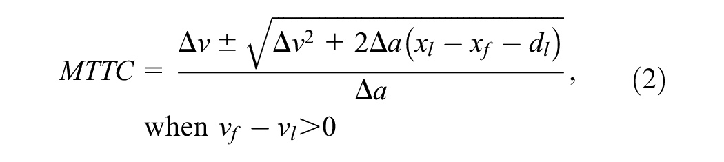
where
Deceleration rate to avoid crash (DRAC): DRAC measures the following vehicle’s deceleration rate that must be used to avoid a collision with the leader vehicle. Equation 3 is used in calculating DRAC.

Some events may not indicate conflict, so events with TTC or MTTC values less than 4.0 s and DRAC greater than 0 m/s2 are used to identify traffic conflict from normal/non-conflicting interactions ( 12 ).
Conflict Sampling Approaches
In EVT models, BM and POT methods are widely used for sampling extreme occurrences, which are subsequently fitted to extreme value distributions. POT was more accurate and reliable than BM in estimating crashes with a limited observation period ( 20 – 22 ). From the literature review, the premise of unsupervised ML anomaly detection methods can be used to identify extreme traffic conflicts as anomalies. This study used unsupervised ML-based anomaly detection methods in addition to POT as a sampling approach.
POT Sampling Method
The POT approach identifies all observations that exceed a specified threshold as extreme events to fit the extreme value distribution ( 20 ). In the EVT model, POT extremes are modeled using the generalized Pareto distribution (GPD) ( 41 ). If X1, X2…, Xn are a sequence of independently and identically distributed random conflict observations, the distribution function for conflict values X over a high threshold u (X > u), can be written as Fu(x) = Pr(X - u ≤ x| X > u). Mathematically, the GPD function can be written as follows:

where
ML-Based Sampling Methods
Anomalies are defined as uncommon traffic events that differ from normal traffic events based on adopted criteria ( 29 ). In our study, anomalies are extreme traffic conflicts used to predict the crash risk. For example, a TTC of more than 4.0 s allows a car enough time to change its speed or course to avoid a crash. On a high-speed interstate, however, a TTC value of less than 4.0 s might not be enough time, suggesting a possible conflict. Based on a previous study ( 12 ), events with TTC or MTTC values of less than 4.0 s and a DRAC greater than 0 m/s2 are used to identify traffic conflicts from normal/non-conflicting interactions in our study. We then categorized traffic conflicts with extreme values as anomalies. Extreme values are those that fall either above the threshold (for DRAC) or below the threshold (for TTC and MTTC).
Isolation Forest (iForest)
The isolation forest (iForest) is an ensemble algorithm based on decision trees, where a forest is formed by multiple trees. The algorithm’s core concept is that observations with distinct characteristic values will be isolated sooner during the partitioning process. Therefore, the likelihood of those points being anomalies is considerable because the trees of the random forest generate a shorter path length ( 27 ).
Mathematically, let X = {X1, X2,…, XN} represent traffic conflict observations. X0 is a subset of those observations used to construct an isolation tree (iTree). The iTree divides the data set recursively by randomly selected attributes and splits until nodes contain either single observations or identical attribute values. Anomalies have shorter path lengths from the root to the final node because their unique attributes lead to quicker isolation. Trained iTrees use these paths to compute anomaly scores, which helps differentiate anomalies from normal observations, akin to the structure of a binary search tree and an unsuccessful search termination ( 27 ). In iForest, h(x) represents the average path length to isolate an observation. It is compared with c(n), the average path length for a binary search tree, to determine the anomaly score. A shorter h(x) relative to c(n) indicates a likely anomaly.

where H is the Harmonic number, and n represents the number of observations or data points in the data set used to construct the isolation tree. The anomaly score can be calculated by normalizing the h(x),

The average of the anomaly scores h(x) produced by a group of isolation trees is represented by the function E(h(x)). Based on the anomaly score, if s is close to 1, the observation is a probable anomaly, and if s < 0.5, it is a normal event. If there are no noticeable anomalies in the sample, all observations have s≈ 0.5 ( 27 ).
One-Class Support Vector Machine (OCSVM)
A support vector machine (SVM), initially created for binary classification, has applications in anomaly detection. Here, all observations are considered part of a single class. OCSVM constructs a hyperplane (or higher-dimensional equivalent) encompassing most normal data points, maximizing the margin from the closest data points (support vectors) to the hyperplane ( 28 ).
Let X = {X1, X2,……., XN} represent the traffic conflict observations, where N is the total count of observations. Assume Фx is a mapping function that transforms Xi from the input space to the feature space F. In this feature space, a linear decision boundary (a hyperplane) f(x) is defined as
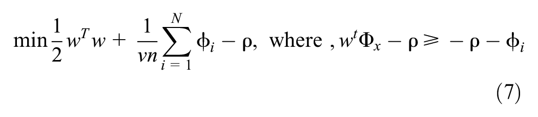
where
This study explored other ML anomaly detection methods: minimum covariate determinant (MCD) and local outlier factor (LOF). MCD measures the distance between the data center and each traffic conflict value, considering the data distribution’s shape ( 42 ). LOF identifies anomalies by assessing how much an observation deviates from the local density of its neighbors, detecting those with lower density compared with nearby points ( 43 ). These methods are described in the corresponding references ( 42 , 43 ). We minimized the method description because these methods did not provide better accuracy than POT.
Standard validation methods (i.e., splitting data into testing and training) are applicable for the development of supervised learning–based ML models using labeled data. In unsupervised ML models with unlabeled data, standard validation measures cannot be applied as ground truth data are not available to compare ( 44 – 50 ). Since the data used in our study was unlabeled, unsupervised ML models were developed through hyperparameter tuning by testing various configurations to find the best-fit model that provides stable, meaningful, and consistent results ( 44 ). Based on past studies ( 44 , 51 , 52 ), we trained and tweaked the parameters systematically to optimize our chosen measure of minimizing the false detection (where data is wrongly detected as an anomaly or a non-anomaly).
The parameters of the OCSVM and iForest models were iteratively tuned. In OCSVM, the parameters to be tuned are nu, tolerance (tol), gamma, and the kernel function. The hyperparameter nu modifies the trade-off between slack penalties ϕi and the hyperplane f(x) margin, which regulates the proportion of data considered outliers. The tolerance hyperparameter regulates the convergence during optimizing parameters w and ρ. The hyperparameter gamma affects the kernel function, which in turn influences the mapping Φ(x) and the shape of the hyperplane ( 53 ). After tuning, the final value of the nu parameter was set to 0.15 and 0.25 for MTTC and DRAC, respectively. The tolerance value was set to 0.001. For the OCSVM model, the radial basis function (RBF) kernel function was used with the gamma value set to auto. On the other hand, for iForest, the number of trees for partitioning, contamination rate, and maximum sample hyperparameter were tuned. The hyperparameter number of trees for partitioning affects E(h(x)), representing the average path length across all trees. The hyperparameter contamination determines the cutoff for anomaly scores s(x,n). The maximum sample hyperparameter affects c(n), which standardizes path lengths among subsamples ( 53 ). After tuning, the number of trees was set to 120, and the contamination rate was set to 0.15 and 0.25 for MTTC and DRAC, respectively. The maximum sample hyperparameter was set to auto. The ML models used one feature (i.e., TTC, MTTC, or DRAC) at a time to find the threshold between anomaly and non-anomaly. Thus, the dimensionality was one in our ML models.
Crash Risk Estimation Approach
Bivariate Generalized Pareto Distribution (BGPD) of EVT
If {(x1, y1), (x2, y2), …} represents independent observations of a random vector (X, Y) with a joint distribution function denoted as F (x, y), where each pair (xi, yi) corresponds to a specific observation of the variables X and, the bivariate threshold excess model is employed to approximate the joint distribution F (x, y) on regions defined as x > ux, y > uy, where the thresholds ux and uy are sufficiently large. For large thresholds, each marginal distribution of F can be approximated by a univariate GPD, with (σx,ξy) and (σx,ξy) as respective parameters ( 23 ).
The bivariate GPD is commonly expressed using the standard Fréchet distribution, which can be derived through the transformations in Equation 8 (54),
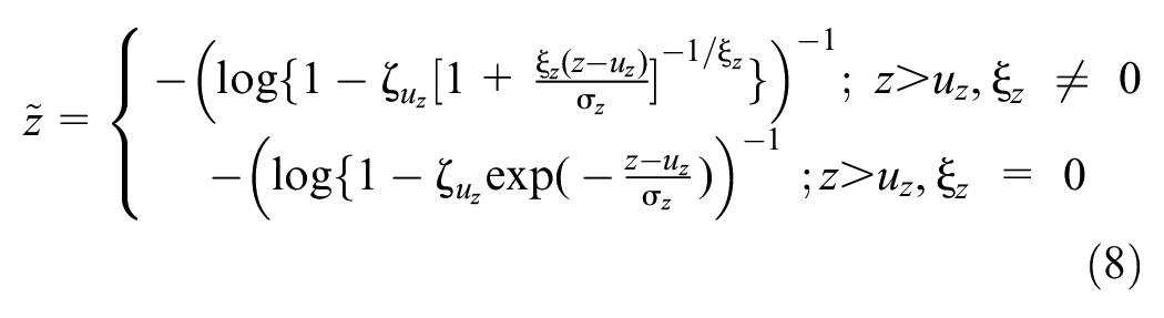
where
z is either the x or y of the original margins,
(X, Y) are the independent observations of conflict indicators (TTC and DRAC, MTTC and DRAC) belonging to a joint distribution.
The parameters (σz, ξz) can be estimated using maximum likelihood estimation.
After the transformation of both margins, both transformed extremes can be modeled by,

where V is the component measure function and
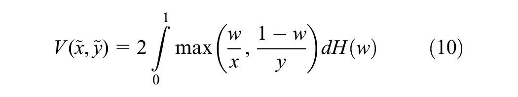
where H (also known as the spectral measure) is a distribution function defined on the interval [0, 1], satisfying the constraint,

Equation 9 provides a valid limit for any distribution function H, defined on the interval [0, 1] in Equation 10, and satisfies the mean constraint specified in Equation 11. However, this will lead to Equation 10 giving rise to a vast range of possible classes of limits ( 23 ). As a result, bivariate distributions become difficult as this will give rise to nearly infinite parametric forms. One way to address this issue is by using specific parametric distributions, such as the logistic family for H, which results in sub-families of distributions for G ( 23 , 41 ). For the logistic model, the spectral density h(w) for the distribution can be presented as,

and

Thus, Equation 9 takes the form,
Parameter α is used to measure the strength of dependence, where α→ 0 indicates complete dependence and α = 1 represents complete independence. The parameter α of the logistic family of parametric distributions quantifies dependence between the random variables at an extreme level ( 42 ).
Various parametric families, such as asymmetry logistic, asymmetry negative logistic, bi-logistic negative logistic, negative bi-logistic, and Husler–Reiss, can be used to model bivariate extreme value distributions ( 23 ). The logistic model is widely used because of its straightforward structure, minimal number of parameters, and flexibility in representing all levels of dependence ( 23 , 54 , 55 ).
Drawing inferences from bivariate excess models can be complicated. While both components in a bivariate pair may surpass their respective thresholds, it is important to note that neither might exceed the specified thresholds. Whether x or y exceeds their respective threshold, four cases arise ( 41 ),
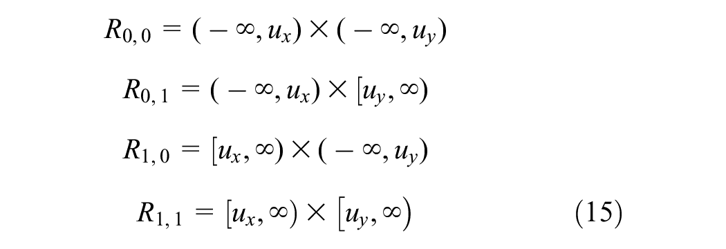
For instance, a point
Setting a very low threshold could undermine the GDP’s theoretical expectation. Conversely, a very high threshold could result in too few extreme events, leading to higher variance in parameter estimates. Therefore, it is crucial to select a threshold that is reasonably low/high enough to maintain a good model approximation ( 41 ). The threshold is generally selected using the mean residual life plot, and the threshold stability plot, and guides for the bivariate model fitting can be found in the appendix section of Zheng et al. ( 54 ). More details about the EVT and related likelihood estimations can be found in Coles ( 41 ).
Modeling Conflict Indicators with Bivariate EVT
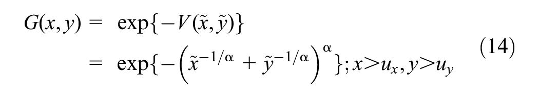
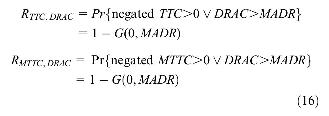
According to the definition, a crash will occur if the value of TTC/MTTC becomes less than or equal to 0 or a negated (negative) TTC/MTTC greater than or equal to 0. However, a crash occurs if the DRAC value exceeds the MADR. According to Cunto and Saccomanno ( 56 ), MADR is the measure of a vehicle’s braking capability and follows a truncated normal distribution MADR∼ Normal (8.45, 1.402) I (4.23, 12.68), where 4.23 m/s2 and 12.68 m/s2 are the lower and upper limits of the distribution. The MADR value is different for different vehicles and depends on factors such as vehicle braking system, pavement, and environmental conditions, and a crash could occur when DRAC exceeds MADR ( 12 , 56 ).
Let E be an event defined by the joint distribution of two random variables
where the estimated bivariate threshold excess distribution from Equation 14 is denoted by G(.).
The number of crashes for both univariate and bivariate approaches can be obtained from the following equation,

where T is the longer period of interest (such as one year) for crash estimation, and the time period (t) represents the shorter period (data collection/observation period).
Results and Discussion
This section presents the findings from bivariate EVT model estimations by applying POT and ML sampling approaches to estimate the rear-end crash risk of the selected segment. During the evening peak hour, there were 8,098 vph (in both directions), with 8.65% being heavy vehicles. The land use pattern of the selected segment was rural, with an annual average daily traffic (AADT) of 100,331 based on the ETRIMS database. Conflicts were identified at the study freeway segment, applying the criteria defined above. The summarized descriptive statistics of the SSMs are as follows: For TTC, there are 327 observations with a mean of 2.16 s and a standard deviation of 1.23; MTTC has 586 observations with a mean of 2.59 s and a standard deviation of 0.97; DRAC includes 410 observations with a mean of 2.51 m/s2 and a standard deviation of 3.57.
Threshold Selection Results
The thresholds for POT were chosen using the method described above. The mean residual life plots and threshold stability plots for TTC, MTTC, and DRAC are shown in Figures 1 and 2, respectively. For DRAC, Figure 1c was moderately linear within the range of 2.5 m/s2 and 5.0 m/s2. The parameter-threshold stability plot was stable between 3.0 and 4.0 (Figure 2c). Based on these observations, 3.5 m/s2 is selected as the threshold for DRAC. The same procedure is followed for the threshold of TTC (−2.3 s) and MTTC (−2.5 s). The
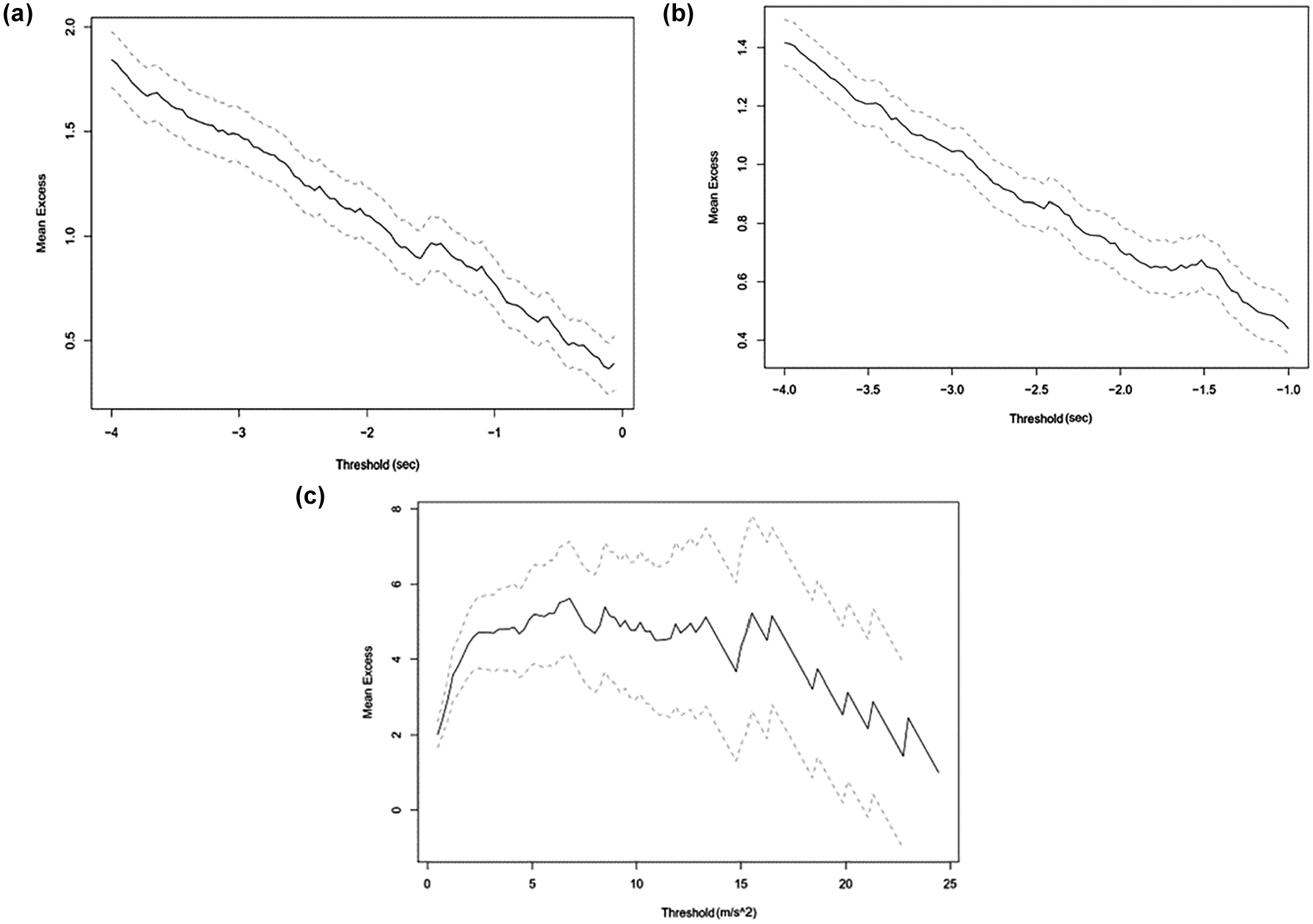
Mean excess plots for (a) time-to-collision (TTC); (b) modified time-to-collision (MTTC); and (c) deceleration rate to avoid crash (DRAC).
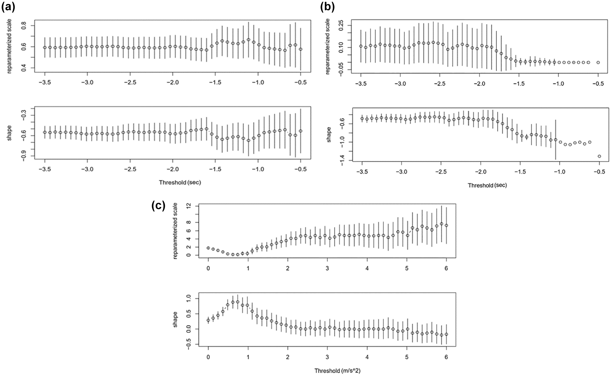
Threshold stability plots for (a) time-to-collision (TTC); (b) modified time-to-collision (MTTC); and (c) deceleration rate to avoid crash (DRAC).
The sampling approaches, such as the POT and ML approaches, identify the threshold necessary for modeling EVT’s GPD. The previous section’s discussion underscores the necessity of selecting proper thresholds, as an improper threshold will lead to bias and variance in the results. However, specifying a threshold in POT for extremes is inherently arbitrary, as neither mean residual life plots nor assessments of parameter stability plots can remove subjectivity from choosing suitable thresholds. These plots are employed initially in selecting the threshold values, where the appropriate thresholds were identified based on minimizing crash prediction errors iteratively ( 3 ). ML-based approaches can reduce this subjectivity by distinguishing anomalies or extremes from normal or non-extreme values. For instance, an SSM value is labeled as an anomaly or normal based on each approach’s anomaly score criteria. The anomalies’ lowest (negated SSMs) or highest value is taken as the threshold.
Bivariate EVT Model Results
The result of the bivariate EVT with the POT approach is given in Table 1. Model goodness of fit can be expressed with the QQ plot and density plot of the marginal distribution of the individual SSM, the Pickands dependence function plot, and the spectral density plot of the logistic distribution function ( 22 , 59 ). Figures 3 and 4 show the QQ, dependence function, and spectral density plots for the MTTC and DRAC models based on the POT approach. The QQ plot shows that the quantiles follow the straight line closely, suggesting that the model fits the data well. The spectral density and the dependence function plot show the goodness of fit for the bivariate model. The spectral density displays a flat profile with peaks at 0 and 1. The peaks depict scenarios where only one component is extreme, and the center (t = 0.5) relates to components reaching extreme values simultaneously. The dependence plot, exhibiting symmetry around t = 0.5, suggests a well-fitted model, with the non-parametric and parametric lines closely aligned, indicating weak dependence ( 22 , 59 ). The spectral density plot would have displayed a peaked curve if the variables were strongly dependent. Also, the dependence function (solid line) plot would have approached the lower end of the triangular region’s (dotted line), indicating that they are completely dependent, and thus, the bivariate MTTC and DRAC model has a good fit. The dependence parameter (α) from Table 1 is approximately 0.99, suggesting weak dependence, and is reasonable given the absence of crashes during the data collection period. If crashes had occurred, there would have been strong dependence at extreme levels, resulting in a smaller value of α ( 22 , 59 ).
Parameter Estimations Applying Bivariate POT and ML Approaches
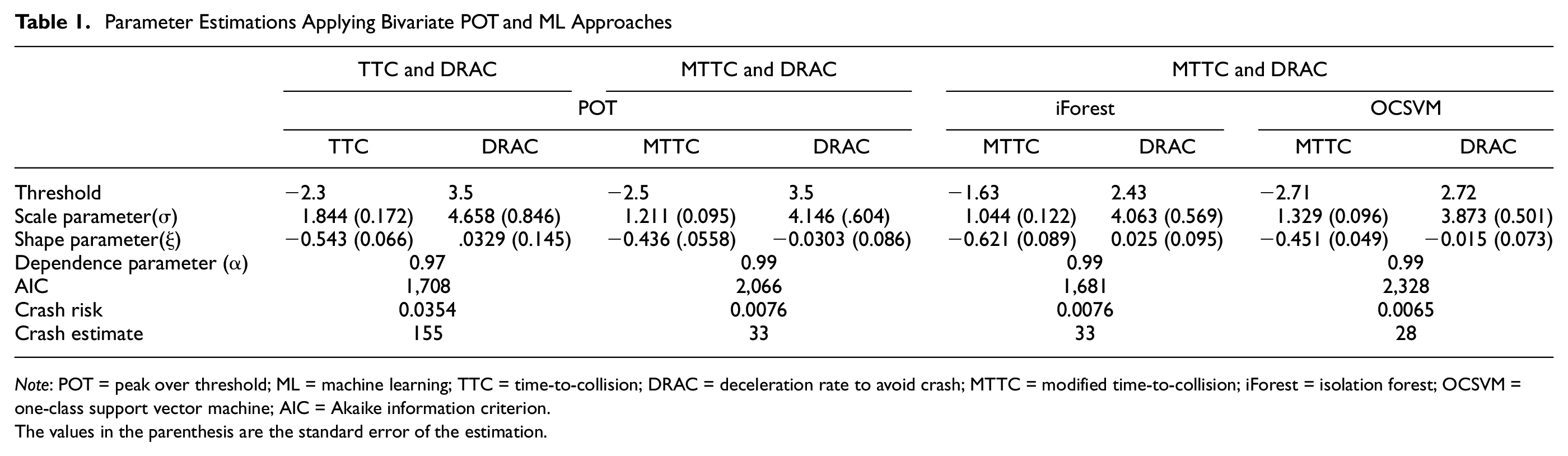
Note: POT = peak over threshold; ML = machine learning; TTC = time-to-collision; DRAC = deceleration rate to avoid crash; MTTC = modified time-to-collision; iForest = isolation forest; OCSVM = one-class support vector machine; AIC = Akaike information criterion.
The values in the parenthesis are the standard error of the estimation.
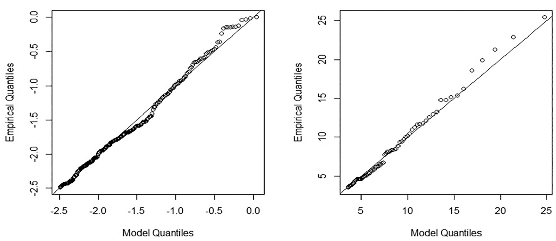
QQ plot of modified time-to-collision (MTTC) (left); and deceleration rate to avoid crash (DRAC) (right).
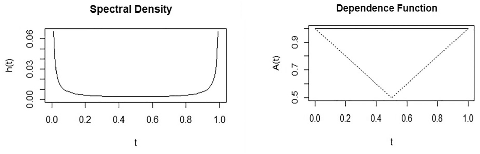
Spectral density and dependance function plot for modified time-to-collision (MTTC) and deceleration rate to avoid crash (DRAC) combination for peak over threshold (POT) approach.
The SSM combinations used in bivariate modeling were (i) TTC and DRAC, and (ii) MTTC and DRAC. Using a combination of complementary traffic conflict indicators, one based on proximity (i.e., MTTC) and another based on evasive actions (i.e., DRAC), provides a more comprehensive understanding of aspects that contribute to crashes, compared with relying on only one SSM indicator ( 11 ). Considering 23 reported rear-end crashes per year, the MTTC and DRAC model combination gave the closest estimate of 33 based on the POT approach.
As the MTTC and DRAC combination provided the best estimate using the POT approach, ML-based sampling, and EVT models were developed for this combination of SSMs. The results of bivariate EVTs with ML sampling approaches are presented in Table 1. As shown in Table 1, the OCSVM sampling method provided the best crash estimate of 28, followed by the iForest sampling method’s crash estimate of 33. The crash estimates by three (POT, iForest, OCSVM) for the MTTC and DRAC combination are within the 99% confidence interval of the observed crashes. The confidence interval (CI) of the observed crash and the CI of the estimated crashes of the bivariate POT and ML models and their corresponding threshold values are shown in Table 2. The overestimation and wider confidence interval could be a result of the pronounced variability of EVT estimates given the short observation period ( 23 , 25 ).
Confidence Interval for Estimated and Observed Crashes
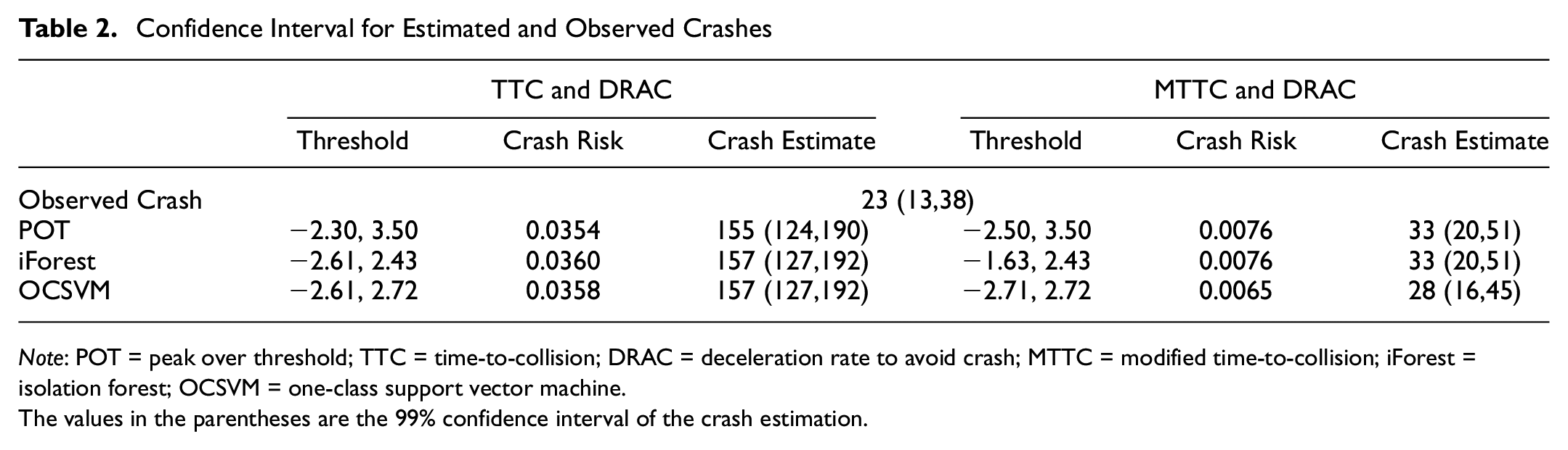
Note: POT = peak over threshold; TTC = time-to-collision; DRAC = deceleration rate to avoid crash; MTTC = modified time-to-collision; iForest = isolation forest; OCSVM = one-class support vector machine.
The values in the parentheses are the 99% confidence interval of the crash estimation.
From the sampling approaches adopted in this study, the OCSVM performed better than POT and iForest. The absolute percentage difference between the estimated crash frequency and the observed crash frequency, and the 99% confidence interval, were used as the performance measure to identify the best-performing model. The absolute percentage differences between crash estimates and observed crashes applying POT, iForest, and OCSVM approaches with EVT were 43.5%, 43.5%, and 21.7% for the MTTC and DRAC models, respectively. Although the crash estimates of the three approaches were within the 99% confidence interval of the observed crashes, the OCSVM approach had a 21% higher accuracy compared with the POT and iForest approaches. Figure 5 shows the comparison of crash estimates for different sampling approaches.
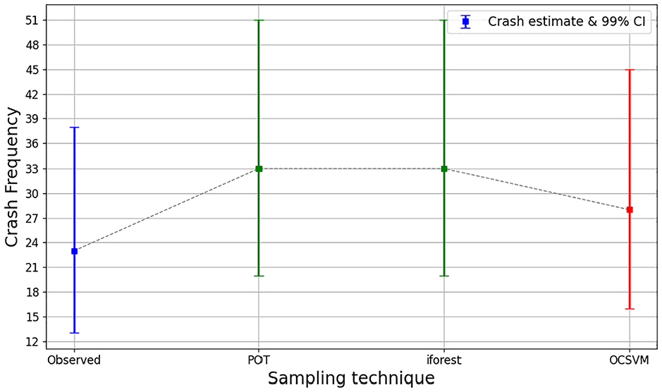
Comparison of crash estimates by sampling approaches for modified time-to-collision (MTTC) and deceleration rate to avoid crash (DRAC).
Using a kernel function, OCSVM transforms input data into a high-dimensional feature space and constructs a decision function to separate normal events from anomalies with maximum margin, and this approach effectively distinguishes normal patterns from anomalies by identifying high-density regions for normal data ( 28 ). Furthermore, the radial basis function (RBF) kernel used in OCSVM is widely used to manage complex data distributions and effectively model non-linear decision boundaries ( 60 ). These capabilities likely contributed to the better performance of the OCSVM in detecting traffic conflict extremes. The performance of iForest can be attributed to its robustness in handling masking and swamping effects and clustered anomalies ( 27 ). These findings show that MTTC and DRAC can be a better bivariate combination to estimate rear-end crash risk in freeway segments, and the OCSVM sampling approach combined with MTTC and DRAC can be an effective modeling framework for freeway crash estimation.
ML methods have become increasingly important in traffic safety studies and prediction because they can model complex functions ( 61 ). Prior research has also demonstrated the potential for improved outcomes from combining statistical and ML techniques. For instance, Wang et al. ( 62 ) combined statistical techniques such as autoregressive integrated moving average (ARIMA) with ML-based SVM to provide improved prediction accuracy for time series forecasts for short-term traffic flow. Xie and Choi ( 63 ) reported similar improvements in long- and short-term traffic flow prediction accuracy by combining statistical and ML neural network (NN) methods for real-time and historical data. This study demonstrated that ML-based sampling methods combined with statistical methods (i.e., EVT) can be used for conflict-based safety studies to improve crash risk estimation accuracy compared with the traditional POT sampling method. Proactive safety evaluation combining ML and EVT without reliance on slow accumulation of crash data can provide accurate results and assist transportation engineers in taking action to maximize safety outcomes. This study’s framework shows that combining the ML method (OCSVM) and statistical method (EVT) yields the most accurate crash estimates. Applying the combined methodology (ML and EVT), practitioners can implement proactive mitigation measures based on conflict measures and estimated crash risk at the newly constructed facility with or without a limited historic crash record. Various data collection strategies, such as lidar or drones, can extract the traffic characteristics data needed to identify and assess spatiotemporal characteristics of conflicts under different traffic conditions ( 64 ). While more data or an observation period can improve accuracy, it requires more data collection and processing resources.
Limitation and Future Direction
Several potential future research directions were identified based on the limitations of this study. This study did not consider the MADR distribution relevant to the specific site and was adopted from a past study by Cunto and Saccomanno ( 56 ). Future research could focus on incorporating appropriate MADR distribution values that accurately reflect the study segments to improve crash estimation accuracy further. In addition, field traffic data collection and analysis over a longer period (compared with one peak hour data used in this study) could improve the estimation. Also, data from different seasons and weather conditions can be used to develop more robust models. Moreover, ML-based anomaly detection methods combined with EVT in this study can be applied using data from additional locations to investigate model/method transferability. Since many modern vehicles are equipped with new technology (i.e., different driver assistance systems), future research could explore/investigate the impacts of these technologies on rear-end crash risk.
Conclusion
This study estimates the rear-end crash risk of a freeway segment by developing bivariate EVT models. Unsupervised ML approaches (iForest, OCSVM) were used as sampling approaches in addition to the conventional POT approach. Selecting a threshold in the POT method for extremes is subjective, as diagnostic plots do not fully resolve this arbitrariness. ML methods can reduce this subjectivity by distinguishing between normal and extreme events. Unsupervised ML anomaly detection identifies rare patterns in unlabeled data based on the assumption that anomalies significantly differ from typical events. Prior research highlighted improved outcomes by combining statistical and ML methods. The uniqueness and contribution of the study are that the inclusion of the ML method led to higher accuracy in crash estimation. The YOLOv8 and Deepsort algorithms, together with the DataFromSky Viewer software, was used to extract traffic volume, headway, speed, acceleration, and type of vehicle from recorded video data to calculate three conflict indicators: TTC, MTTC, and DRAC. The results show that the bivariate SSM combination of MTTC and DRAC produces the best estimate. The crash estimate of the MTTC and DRAC model with the POT sampling approach falls within the 99% confidence interval of the observed crash. Like the POT approach, two ML sampling approaches, iForest and OCSVM, also performed better for the MTTC and DRAC combination. However, the OCSVM sampling reduces crash estimation errors by 21% compared with the POT and the iForest sampling approaches. These results indicate that the OCSVM-based sampling approach with EVT modeling is an effective framework for freeway crash estimation. This integrated ML-based OCSVM sampling and statistical EVT approach for crash estimation can be used for site-specific safety evaluations, especially roadway segments with limited crash data. Data collection strategies, such as lidar or drones, can assist in obtaining essential traffic characteristics needed for detecting conflicts and analyzing their spatiotemporal factors. Integrating ML and EVT without needing prolonged crash data, proactive safety evaluation enables transportation engineers to make impactful safety decisions.
Footnotes
Author Contributions
The authors confirm contribution to the paper as follows: study conception and design: M.T. Ashraf, M.I. Khan, K. Dey; data collection: M.I. Khan, M.T. Ashraf; analysis and interpretation of results: M.I. Khan; draft manuscript preparation: M.I. Khan, M.T. Ashraf, K. Dey, P. Kar, S. Mishra, M. Hunt, M. Golias. All authors reviewed the results and approved the final version of the manuscript.
Declaration of Conflicting Interests
The author(s) declared the following potential conflicts of interest with respect to the research, authorship, and/or publication of this article: Sabya Mishra is a member of Transportation Research Record’s Editorial Board. All other authors declared no potential conflicts of interest with respect to the research, authorship, and/or publication of this article.
Funding
The author(s) disclosed receipt of the following financial support for the research, authorship, and/or publication of this article: This research was funded by the Tennessee Department of Transportation and the Federal Highway Administration.
Data Accessibility Statement
Some or all data, models, or code that support the findings of this study are available from the corresponding author on reasonable request.
This paper reflects the authors’ views and does not necessarily reflect the views of the Tennessee Department of Transportation or the Federal Highway Administration.