Modeling the Effects of Driver and Road Geometric Characteristics on Consecutive Horizontal Curve Perception

Abstract

Driver errors are the major contributors to run-off-road crashes on horizontal curves. Hence, understanding driver perception of horizontal curves is essential for improving road safety. This study examined the combined effects of driver characteristics such as, age, driving experience, annual distance driven, driver type, education, eyeglass use, and geometric features such as radius of preceding curve (R_P), difference between radii of preceding and succedding curves (ΔR), deflection angle (DA) on consecutive horizontal curve perception. A questionnaire survey was conducted using simulated images of various curve combinations of four-lane rural highways. Ninety-five male drivers examined the images for differences between consecutive curves and responded in a dichotomous (Yes/No) format. Preliminary analysis identified no significant relationship between driver responses and operating speed. Additionally, image- and video-based presentation methods for examining consecutive curve perceptions were found to be statistically comparable. Driver responses were modeled using mixed-effects logistic regression, identifying ΔR, R_P, Annual distance driven×ΔR, Annual distance driven×DA, and Driving experience×ΔR as significant predictors. The developed model evaluates geometric consistency based on the probability of correctly perceiving curve differences. For existing alignments, curve combinations with R_P = 300-400 m and ΔR = 50–150 m (e.g., threshold probability < 0.5) were deemed perceptually inconsistent and recommended for treatments like speed signage or chevron signs. For new designs, combinations with R_P = 150–300 m, ΔR = 150–300 m, and DA = 30–90 degrees were identified as perceptually consistent. The findings support safety policy recommendations, including graduated driver licensing for drivers with ≤10 years of experience and supervised training for drivers covering ≤1,000km annually.

Keywords

driver characteristics driving experience horizontal curve perception rural highway vision zero road safety

Road safety is a global issue, with an estimated 1.3 million fatalities and 20–50 million injuries occurring annually ( 1 ). Multiple nations have adopted the “Safe Systems Approach (SSA)” to design roadway systems that aim for zero fatalities. A core principle of SSA is safe people that acknowledge human errors as inevitable and fatalities as ethically unacceptable in a well-designed roadway system ( 2 , 3 ). This user-centric approach considers human capacities and limitations, promoting road and vehicle designs that adapt to these factors while enhancing road user skills through education and training. Speeding is a major contributor to road fatalities across all vehicle types, particularly in high-risk locations such as horizontal curves, merge ramps, and diverging ramps ( 4 ). Excessive speed on high-speed highways often leads to fatal run-off-road (ROR) crashes ( 5 , 6 ). It was reported that about 62% of ROR crashes occurred on divided roads, while 40% occurred on undivided roads ( 5 ). Among these, 60–70% of fatal crashes occurred on horizontal curves, where drivers face cognitive and perceptual challenges. SSA promotes speed management through a combination of vehicle safety technologies (e.g., anti-lock braking systems), self-explanatory road designs, speed limit settings based on human crash tolerance, and strict enforcement measures. The long-term target of SSA as a global road safety policy is “Vision Zero,” which has been instrumental in reducing road fatalities ( 3 , 7 , 8 ). For instance, Sweden witnessed a 60% decrease in car-user fatalities during the period of 2000 to 2010, with further declines after the implementation of Vision Zero guidelines ( 7 , 8 ). In India, Vision Zero initiatives aim for zero fatalities by the year 2030 but remain limited to urban areas. This could be attributable to challenges in rural areas, such as mixed traffic conditions, conventional road design, and insufficient enforcement ( 9 ).

A combination of driver, vehicle, and road characteristics influences ROR crashes. In fact, more than 90% of crashes are attributable to driver errors ( 10 , 11 ). Driving is a dynamic and complex activity involving visual, cognitive, and manual tasks ( 12 ). A visual task is a primary task requiring drivers to sense geometric and roadside information visually. This information is stored and processed through a cognitive mechanism to perform manual operational tasks, such as operating the steering wheel and accelerator. The process of information processing depends on the driver’s cognitive ability, which can vary based on memory capacity, attention span, concentration, and so forth. ( 12 , 13 ). As a result, some drivers can undertake vehicle operational tasks slowly while others can do them quickly based on their individual characteristics, such as age, gender, education, and experience ( 14 ). The ability to process visual information, such as the curvature and deflection angle of an upcoming curve, is critical for safe navigation. Drivers’ cognitive abilities determine how well they interpret and respond to this information ( 14 ). When approaching horizontal curves, drivers need to assess the road geometry and adjust their behaviors (e.g., speed and lateral position) accordingly. They may face challenging situations when their cognitive abilities do not match the demands of the curve, possibly owing to high speed, inexperience, distraction, or poor perception ( 15 ). These situations may increase the risk of ROR crashes when horizontal curves are closely spaced (i.e., tangent length < 200 m) ( 16 ). On consecutive horizontal curves, drivers may struggle to perceive differences between the curves as their memory of the preceding curve influences their perception of the successive curve ( 17 , 18 ). Additionally, prior driving experience on similar road geometries may influence drivers’ perceptions of horizontal curves. For instance, a driver may underestimate the difference between the two consecutive curves (i.e., a milder curve followed by a sharper curve) and consequently perceive the sharper curve as milder ( 19 – 21 ). This misperception can increase the likelihood of fatal ROR crashes.

Examining the effects of potential factors on horizontal curve perception through visual cues (e.g., sharpness, deflection angle, visibility) is critical to understanding driver behaviors on horizontal curves. Drivers are subjected to a complex driving environment whereby both road and driver interact. Drivers not only encounter road geometric characteristics (e.g., curve radius, deflection angle) but their driving behaviors are also influenced by their individual factors (e.g., age and experience) ( 22 ). Furthermore, horizontal curve perception was rarely studied for Indian driving conditions ( 20 ). Therefore, this study aims to utilize a comprehensive approach integrating driver and road geometric characteristics for examining their individual and interaction effects on consecutive horizontal curve perception. These factors would be instrumental in engineering applications and policymaking to reduce fatal ROR crashes in India. The specific study objectives are defined as follows:

i. To examine the combined effects of driver and road geometric characteristics on consecutive horizontal curve perception.

ii. To recommend engineering applications and policy implications using the study findings.

The study findings will help to determine key factors that facilitate design consistency and safety of four-lane divided rural highways in India. The findings will support the development and implementation of road safety policies, complementing Vision Zero.

Background

A literature review was conducted on (i) driver perception and (ii) factors influencing driver perception, to acquire background knowledge and identify research gaps.

Driver Perception

Table 1 summarizes the prior driver perception studies. These studies were primarily conducted in developed nations, such as Canada, the United States, and Italy, and were rarely conducted in India ( 6 , 19 , 21 , 23 – 36 ). In these studies, perceptual measures such as curve sharpness, speed, preview sight distance, and risk were collected ( 6 , 19 – 21 , 23 – 36 ). Data collection was conducted in simulated environments, allowing controlled experimentation while minimizing real-world risks. Driver-perspective models of road scenarios were used and presented using different methods and media (as discussed below). Based on the perceptual measure, the number of road scenario combinations and participants was considered. Several questionnaire response formats were used to record participant responses, including numerical rating scale (e.g., 1–5), dichotomous (e.g., Yes/No), and descriptive comparative scale (“Same sharp as,”“less sharp than,”“more sharp than” the test curve). In horizontal curve perception studies, matching and descriptive comparative scale formats were often used to match and compare test curves against reference curves ( 21 , 23 , 24 , 27 , 28 ).

Table 1.

Summary of Driver Perception Studies

Perceptual measures	Presentation method	Presentation medium	Road scenario combinations	Sample size (number of participants)	Questionnaire response format	Effects of driver and road characteristics examined?	Country	References
Curve sharpness	3D static images	Computer screen	378	68	Dichotomous (Yes/No)	No	India	20
	2D static images, 3D dynamic videos		20	40	Numerical rating scale (1-5)	No	Poland	26
	3D dynamic animations		14	67	Matching	No	Canada	21
	2D line drawings	Projection screen	60	44	Magnitude estimation	No	Australia	25
	3D static images, 3D dynamic videos	Computer screen	80 (40 horizontal curves were modeled with 20 as crest combinations and 20 as sag combinations, 40 reference curves overlapping with flat grade)	91	Descriptive comparative scale (“Same sharp as,”“less sharp than,”“more sharp than” the test curve)	No	Canada	28
	3D static images		36 horizontal curves overlapping with vertical curves, 5 reference curves	80	Descriptive comparative scale (“Same sharp as,”“less sharp than,”“more sharp than” the test curve)	No	Canada	27
	3D static images, 3D dynamic videos		54	91	Descriptive comparative scale (“Same sharp as,”“less sharp than,”“more sharp than” the test curve)	No	Canada	23
	3D static images		54	90	Matching	No	Canada	24
	3D dynamic videos	Driving simulator	18 combinations of vertical crest curve and horizontal curves, 18 combinations of vertical sag curve and horizontal curves, 12 horizontal curves overlapping with flat vertical alignment	36	NA	No	Canada	19
Curve sharpness, Discomfort	3D dynamic videos	Driving simulator	12 (3 sag combinations with 3 reference curves and 3 crest combinations with 3 reference curves)	35	NA	No	Italy	6
Speed	2D static images	NA	28	819	Dichotomous (First curve/Second curve)	No	The Netherlands	30
Speed, Safety	3D static images	Computer screen	30	22	Numerical, Numerical rating scale (1-10)	No	Israel	29
Preview sight distance	2D static images, 3D dynamic videos	Computer screen	40	71	Dichotomous (Left/Right)	No	Canada	31
	3D dynamic videos		30	33	Dichotomous (Left/Right)	No	Canada	28
Risk	3D static images, 3D dynamic videos	Driving simulator	36	69	Numerical rating scale (1-10)	No	New Zealand	32
		Computer screen, VR headset	2	146	Numerical rating scale (1-5)	No	United Kingdom	34
Hazard Anticipation	3D dynamic videos	Driving simulator, VR headset	10	36	Dichotomous (miss/hit)	No	United States	33
			6	48	Dichotomous (miss/hit)	Yes	United States	35
Comfort, Safety	3D dynamic videos	Driving simulator	4	42	NA	No	France	36
Consecutive Horizontal curves	3D static images	Computer screen, VR headset	57	95	Dichotomous (Yes/No)	Yes	India	This study

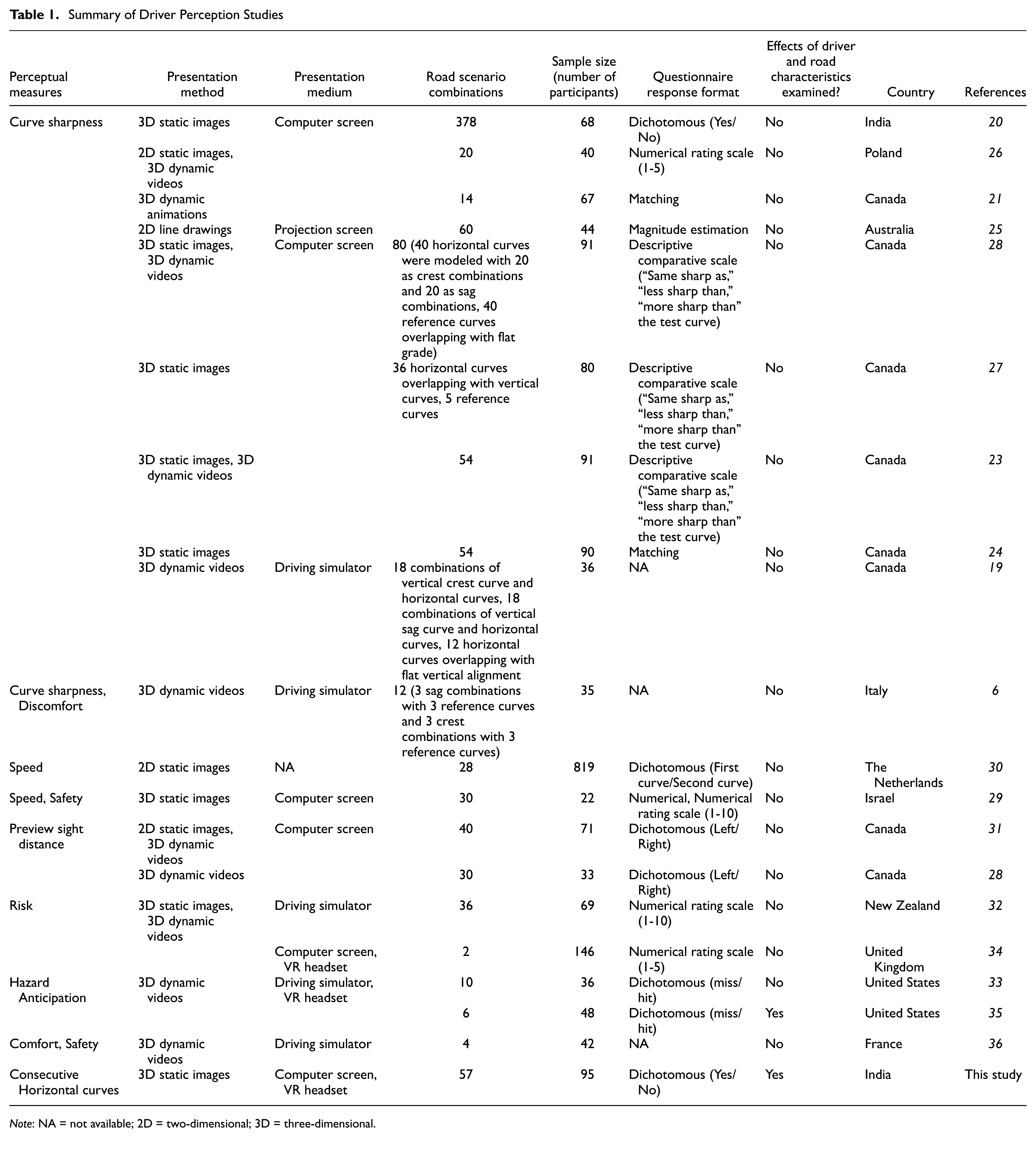
Note: NA = not available; 2D = two-dimensional; 3D = three-dimensional.

Presentation Methods

Researchers conducted questionnaire surveys in simulated environments, where driver-perspective models of road scenarios (e.g., horizontal curve) were presented to participants in two-dimensional (2D) and three-dimensional (3D) forms ( 20 , 26 ). In the 2D form, static line diagrams were often used. In the 3D form, static images and dynamic animations/videos were used, providing a more realistic presentation. Although 3D dynamic videos offered immersive experiences, they might introduce challenges in controlling road alignment parameters and could be time-intensive for comparative analysis ( 21 , 30 ). Conversely, 3D static images provided a cost-effective data collection method and were widely used. Few studies observed that 3D static and 3D dynamic methods yield similar results in collecting drivers' responses to curve sharpness perception ( 23 , 26 , 28 ). However, the findings of those studies were preliminary to draw strong conclusions.

Presentation Media

Researchers presented driver-perspective models of road scenarios to participants through media, such as computer screens, a driving simulators, and virtual reality (VR) headsets. Computer screens and driving simulators were extensively used compared with the limited usage of VR headsets. However, VR headsets have been used in studies related to risk/safety perception to examine drivers’ hazard anticipation and mitigation ( 33 – 36 ). These studies observed that drivers anticipated higher hazards in VR headsets than in driving simulators. This could be attributed to the immersive 3D space provided by VR that allowed drivers to experience road environments with depth perception and head tracking. VR headsets also offer other advantages, such as portability and cost-effectiveness over computer screens and driving simulators ( 35 ). Despite these advantages, VR headsets have few limitations: (i) limited applications in driving research and (ii) motion sickness owing to extended use ( 34 ).

Some driver perception studies examined driver and road geometric characteristics ( 20 , 23 , 24 , 30 , 31 , 35 ). However, most of these studies examined driver characteristics in isolation from road geometric characteristics ( 20 , 23 , 24 , 30 , 31 ).

Factors Influencing Driver Perception

Drivers first identify the upcoming horizontal curve and accordingly adjust their driving behaviors on the curve. Driver behavior on horizontal curves is influenced by their visual perception, which is, in turn, affected by driver characteristics, road geometry, and vehicle characteristics (Figure 1). The visual misperception of horizontal curves may result in inappropriate driver behavior (e.g., speed choices) and fatal ROR crashes on curves. Table 2 presents a summary of prior driver behavior studies, highlighting influencing factors and their groups based on driver characteristics, road geometry, and vehicle characteristics. Among driver characteristics, factors such as age, gender, experience, education, and occupation have been extensively studied ( 15 , 20 , 23 , 24 , 28 , 37 – 49 ). Vision capability has also been examined, as it influences a driver’s ability to interpret visual cues ( 23 , 24 , 28 ). Therefore, age, gender, experience, education, occupation, and vision were selected as the influencing factors for consecutive horizontal curve perception in this study. Prior studies have classified drivers aged from 18 to 30 years as young drivers ( 15 , 38 ). Borowsky et al. ( 39 ), Lehtonen et al. ( 40 ), and Xu et al. ( 41 ) classified drivers with more than 10 years of driving experience as experienced drivers. Chaudhary and Maji ( 42 ) defined drivers with ≤ 1,000 km/year of driving as low-experience drivers. Other studies have also suggested driver classifications based on driver type, education, and use of eyeglasses (40 – 43). Based on these literature considerations, the driver characteristic factors in this study were divided into two groups. Age as young (18–30 years) and old (> 30 years), driving experience as low (≤10 years) and high (>10 years), annual distance driven as low (≤1,000 km) and high (>1,000 km), driver type as non-professional and professional, education as high school and college, and eyeglass use as no eyeglasses and with eyeglasses.

Figure 1.

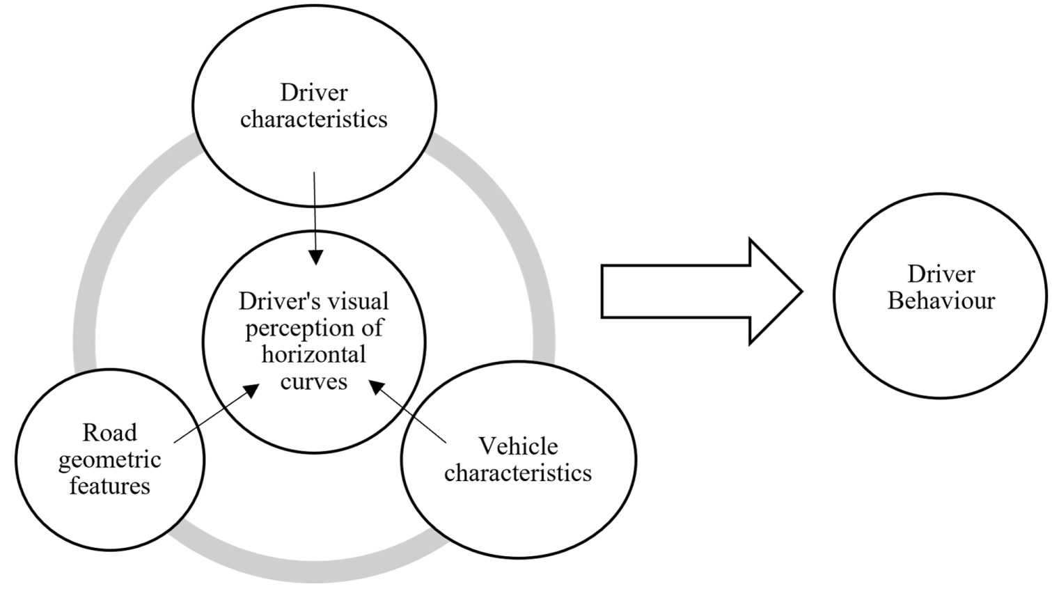
Conceptual framework of factors influencing driver behaviors on horizontal curves.

Table 2.

Summary of Influencing Factors Used in Driver Behavior Studies

Influencing factors	Factor groups	Literature references
Driver characteristics
Age, gender, driving experience, occupation, marital status, education, ethnicity, having children or not, living with spouse, license, annual income, history of chronic disease, frequency of physical exercise every week, eyeglasses use, frequency of driving on rural highways, number of collisions, trips per week	Age: young and oldAge (years): <20, 20–29, 30–39, 40–49, ≥50Gender: male and femaleExperience: experienced, novice/inexperiencedExperience (years): ≤ 2, 3–5, 6–10, 11–15, 16–20, and ≥ 21Experience (year): < 5, 5–10Experience (km/year): low (1,000), mid (1,000–3,000), high (>3,000)Type: professional, unprofessionalEducation: illiterate, primary, intermediate, secondary, universityOccupation: not working, sedentary/professional, manual, businessman, housewife, army/police, studentCar type: four-wheel drive car, small carSeat belt use: yes, noAnnual income (Thousand INR): <200, 200–500, >500Marital status: married, singleTrip type: work, recreationalTrips per week: ≤ 5, > 5	15, 20, 23, 24, 28, 37, 38 –49
Road/geometric features
Curve radius, deflection angle of curve, length of spiral, position of the vertical curve midpoint relative to the horizontal curve, algebraic difference of vertical grades, gradient, curvature, length of curve, superelevation, sight distance, lane width, work zone treatment, traffic, roadway objects, lane configuration, urban/rural environments, curvature, congestion levels	DA: 10-100 degreesSuperelevation: –6% to 6%Gradient: 4%, 8%R: 100 to 700 mLength of curve: 200 mLength of spiral: 50,60, 70, 80, 90 mCurvature: straight, 720 m, and 1500 mCongestion levels: Level of service (LOS) A, LOS C, and LOS E	20, 21, 23–25, 27, 28, 30–32, 44 –46
Vehicle characteristics
Persuasive in-vehicle systems, tire wear, engine power, in-vehicle active accelerator pedal	na	51 –55

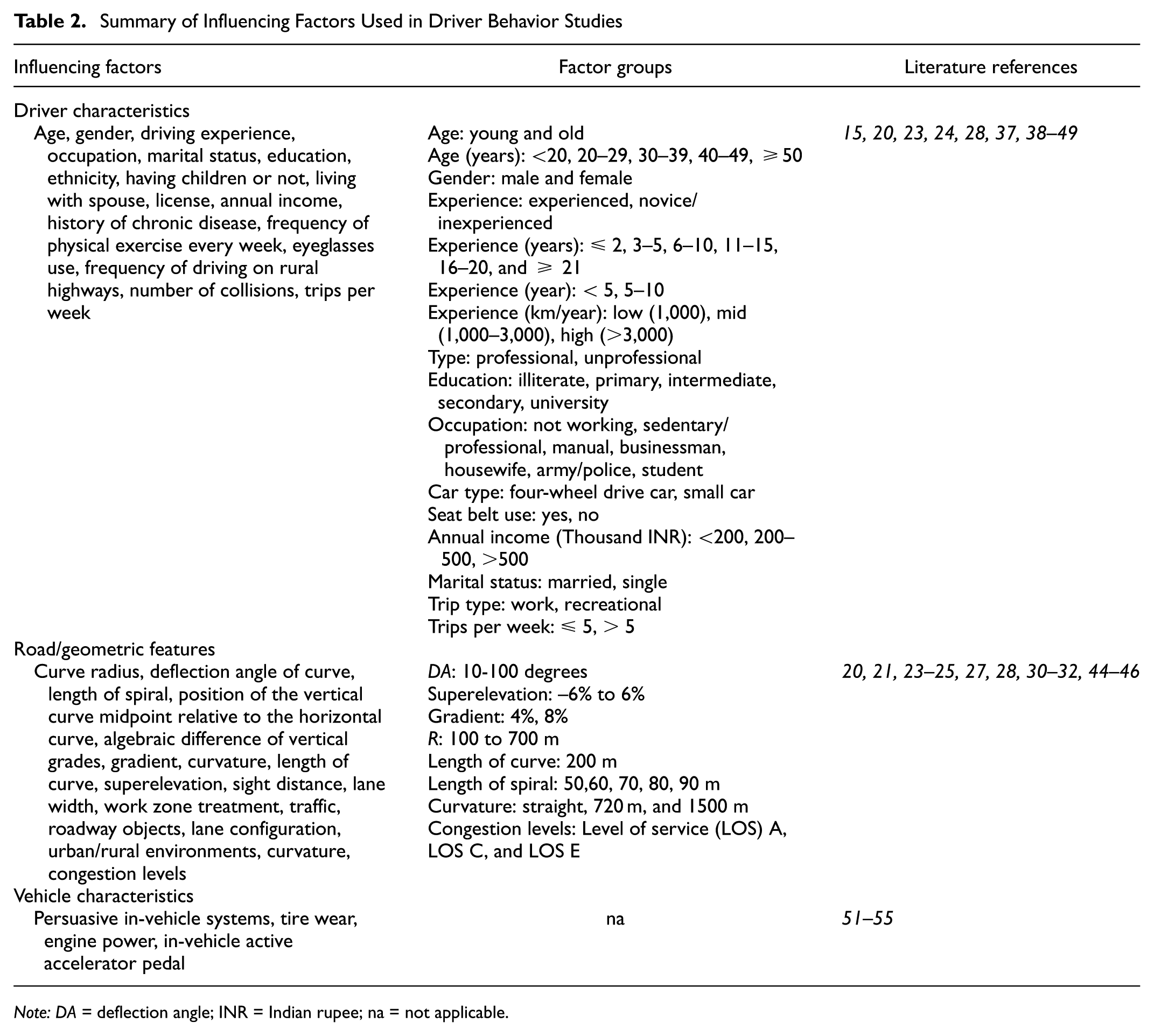
Note: DA = deflection angle; INR = Indian rupee; na = not applicable.

Among road/geometric features, various features, including curve radius (R), deflection angle (DA), lane width, and traffic, were studied in driver behavior research ( 20 , 21 , 23 – 25 , 27 , 28 , 30 – 32 , 44 – 46 ). R and DA are the important geometric features that describe the visual representation of a horizontal curve ( 50 ). Thus, the effects of R and DA on horizontal curve perception could be critical. Some studies examined driver and road/geometric characteristics ( 20 , 23 , 24 , 28 , 44 – 46 ). However, most of these studies examined driver characteristics in isolation from geometric characteristics ( 20 , 23 , 24 , 28 , 46 ). A few studies examined the interaction effects between these factors ( 44 , 45 ). Among driver behavior studies, a few studies also examined vehicular characteristics, such as engine power, tire condition (e.g., wear), and in-vehicle systems (e.g., active accelerator pedal) ( 51 – 55 ). Vehicular characteristics influence driving comfort but have a questionable impact on safety. High-performance vehicles, while offering better speed and torque, are associated with increased risk-taking behaviors ( 50 ). However, the relationship between vehicle performance and driver risk is complex, as driver characteristics primarily determine driver behavior and the likelihood of crashes.

Research Gaps and Novelty

Based on the critical literature review on driver perception and behavior research, notable research gaps were identified, as indicated in Table 1. It is evident from the literature that road geometric design influences drivers’ speed choices and vehicle control, as characteristics such as curve radius, superelevation, and sight distance directly affect them for safe driving. Drivers are the primary users of a roadway system and are subjected to a complex driving environment in which both road and driver interact. Drivers do not simply encounter road characteristics in isolation; their perceptions, decision-making, and behaviors are also influenced by their individual factors (e.g., age and experience) ( 22 ). Moreover, some drivers exhibit accident proneness owing to inherent characteristics, risk perception, or driving behaviors ( 56 ). In driver behavior research, driver characteristics (e.g., age and experience) and road geometric characteristics (e.g., curve radius, deflection angle) were extensively examined. Most of these studies examined driver characteristics in isolation from road/geometric characteristics ( 20 , 23 , 24 , 28 , 46 ). A few of these studies examined the interaction between driver and road/geometric characteristics ( 44 , 45 ). In driver perception research (viz, horizontal curve perception), most studies examined only road geometric characteristics. A few of these studies have investigated driver and road geometric characteristics, but in isolation from road geometric characteristics ( 20 , 23 , 24 , 30 , 31 ). Therefore, the explicit knowledge of combined driver and road geometric characteristics to examine horizontal curve perception is a critical research question. Furthermore, horizontal curve perception was rarely studied in India, which is crucial considering its left-hand driving, heterogeneous traffic flow, and weak lane discipline driving conditions different from those in developed countries ( 9 , 20 ). Therefore, this study contributes to the existing literature by adopting an integrated approach to examine the combined effects of driver and road geometric characteristics on consecutive horizontal curve perception. By simultaneously analyzing these factors, this study aims to provide a more comprehensive understanding of how road design and driver-specific characteristics interact to influence driver behaviors. This integrated approach has significant implications for driver-centered roadway design, the development of advanced driver-assistance technologies, and the formulation of data-driven policy interventions to improve road safety in India. Understanding these interactions will benefit transportation engineers and policymakers in designing roadways that align with driver capabilities, mitigate risk-prone behaviors, and enhance overall driving safety.

Data and Methods

A three-step methodology was utilized to accomplish the study objectives. The first step was the selection of curve geometry, including development of driver-perspective simulated models for collecting driver responses. The second step was the data collection methodology. The third step includes the methods used for developing the driver response model. The detailed study methodology is discussed as follows:

Selection of Curve Geometry

Consecutive horizontal curves are typically designed owing to several constraints, such as topography (i.e., hilly or mountainous), land acquisition, cost, or rehabilitation purposes. Negotiating these curves can be particularly challenging for drivers on four-lane divided highways owing to higher design speeds and increased lateral clearance. Therefore, consecutive horizontal curves of rural four-lane divided highways were considered in this study. Based on the design guidelines ( 50 , 57 ), horizontal curves with radii ranging from 100 to 400 m in increments of 50 m ( 23 ), and curve lengths greater than transition curve lengths were selected. Consecutive curves transitioning from a preceding curve with a larger radius to a succeeding curve with a smaller radius and separated by a short tangent (i.e., tangent length < 200 m) were considered to represent critical geometric combinations. The ratio of the preceding curve radius to the succeeding curve radius was taken as 2:1 (recommended by American Association of State Highway and Transportation Officials [AASHTO] guidelines) or greater to include critical consecutive curves ( 50 ). Curves in the same direction were selected, as those can be more critical because drivers may not anticipate the need for significant deceleration when transitioning from a mild to a sharp curve. If the ratio of a mild curve to a sharp curve exceeds 2:1, drivers may lose control, resulting in ROR crashes ( 50 ). When designing consecutive curves, large differences in deflection angles are typically avoided, particularly on multilane highways, to reduce driver workload and enhance safety. A study has shown that when the change in deflection angles between curves is less than 10 degrees, drivers’ perception of curvature remains largely unchanged (26). Therefore, selected consecutive curve combinations featured two same-direction horizontal curves with identical deflection angles and separated by a short tangent. A consecutive curve combination was represented as “R_P-ΔR” where R_P represents the radius of the preceding curve and ΔR represents the difference between the radius of the preceding curve (R_P) and the radius of the succeeding curve (R_S). A total of 57 feasible consecutive curve combinations were selected having identical deflection angles (i.e., DA_P = DA_S) of 30, 60, and 90 degrees, as shown in Table 3. Using the selected geometries of consecutive curve combinations, driver-perspective simulated models in the form of 3D static images were developed to represent a passenger car traveling at a speed of 100 km/h on the inner lane 50 m before the point of curvature (PC) of the curve. These models were developed in AutoCAD Civil 3D^®, following the methodology used by Sil et al. ( 20 ).

Table 3.

Consecutive Curve Combinations

Deflection angle (i.e., DA_P = DA_S) (degree)	30	60	90
R_P-ΔR (m)	200–50	150–50	150–50
	250–50	200–50	200–50
	250–100	200–100	200–100
	300–50	250–50	250–50
	300–100	250–100	250–100
	300–150	250–150	250–150
	350–50	300–50	300–50
	350–100	300–100	300–100
	350–150	300–150	300–150
	350–200	300–200	300–200
	400–50	350–50	350–50
	400–100	350–100	350–100
	400–150	350–150	350–150
	400–200	350–200	350–200
	400–250	350–250	350–250
		400–50	400–50
		400–100	400–100
		400–150	400–150
		400–200	400–200
		400–250	400–250
		400–300	400–300

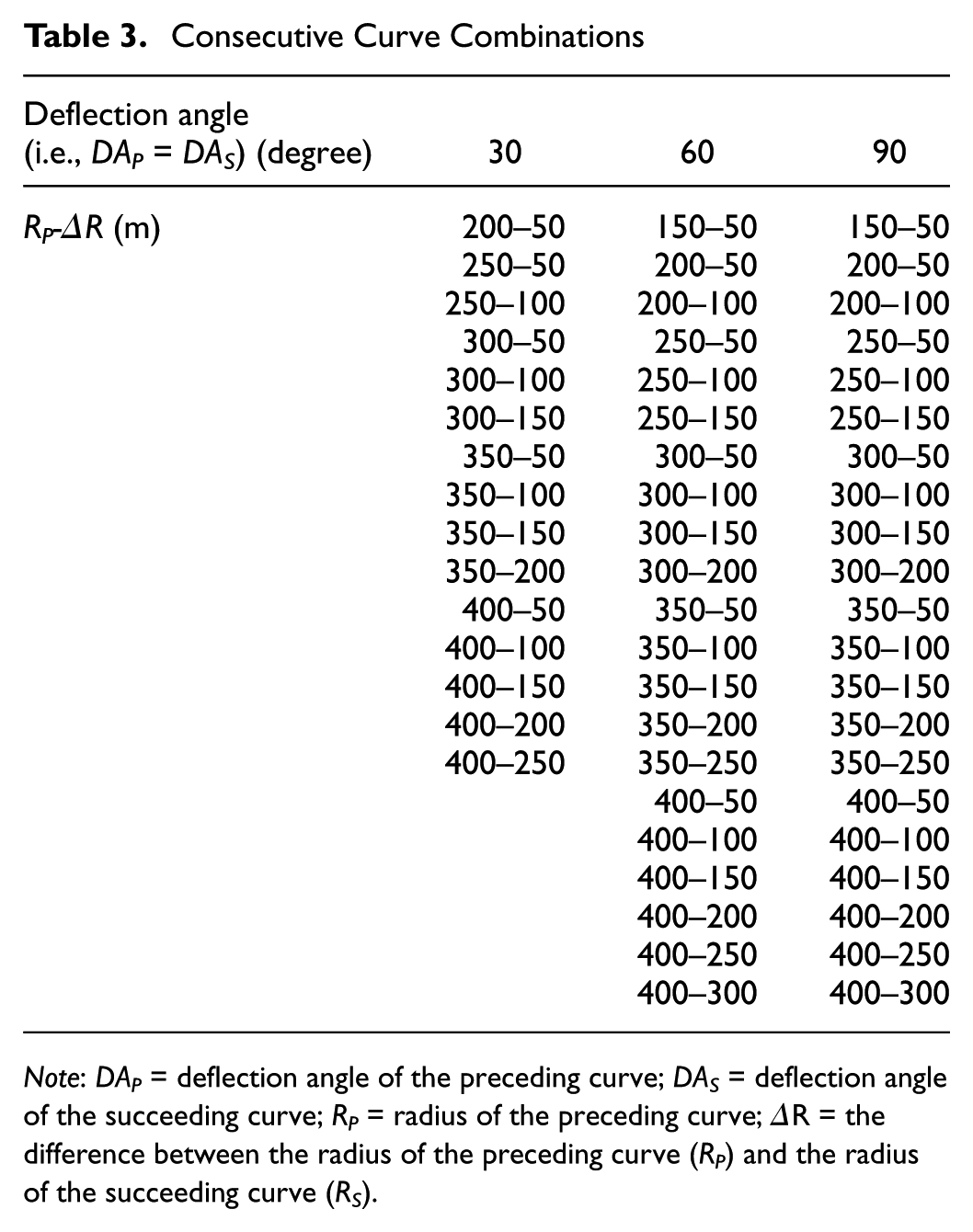
Note: DA_P = deflection angle of the preceding curve; DA_S = deflection angle of the succeeding curve; R_P = radius of the preceding curve; ΔR = the difference between the radius of the preceding curve (R_P) and the radius of the succeeding curve (R_S).

Data Collection

A questionnaire survey was conducted at the traffic engineering laboratories of IIT Indore and IIT Bombay campuses between 2018 and 2022 to collect drivers’ perceptions and demographic data. Drivers available inside the campuses and around the Indore and Mumbai district regions were called based on a valid driving license and a minimum of 2 years of driving experience. A total of 104 drivers, consisting of 101 males and 3 females, participated in the survey. The population of drivers included students, researchers, staff members, visitors, and professional drivers. Participants whose primary occupation was driving were considered professional drivers (43). For the perception data collection, two 3D static images for each of the consecutive curve combinations were vertically arranged in a top-down manner at the center of the Microsoft PowerPoint slides. The background of the slides was made black for visual contrast and focus enhancement, in line with prior studies ( 23 , 24 , 27 , 28 ). The time duration for each consecutive curve combination was set for 4 s (i.e., 2 s for each curve) ( 20 ). A blank transition slide of 2 s duration was inserted between the two consecutive slides. A high-quality video file was created for the PowerPoint slides and presented to drivers on two presentation media: (i) a computer screen and (ii) a VR headset, as shown in Figure 2. Figure 2 illustrates the presentation of two 3D static images of a consecutive curve combination (depicted as preceding and succeeding curves). In the computer screen presentation, drivers were seated at 0.5 to 0.6 m from the screen ( 21 ). In the VR headset presentation, drivers were made to wear the VR headset in a seating position to view the virtual screen. The video player in the VR headset featured a large screen and a wide field of view, offering a virtual theatre-like experience and enhancing visual immersion. Before the main session, a test session of 30 s was conducted to familiarize drivers with the presentation setup.

Figure 2.

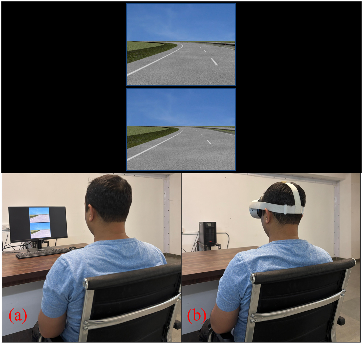
Presentation of three-dimensional (3D) static images of a consecutive curve combination to a driver on a (a) computer screen and (b) virtual reality (VR) headset.

It was observed from the literature review that matching and descriptive comparative scale formats were often used for recording driver responses in horizontal curve perception studies. However, considering the objective of collecting drivers’ perception of the differences in curve combinations in this study, a dichotomous (Yes/No) format was used, in line with Sil et al. ( 20 ). In the main session, drivers were asked to examine differences in consecutive curves (see Figure 2) and indicate whether they perceived any difference by responding in “Yes” or “No.” In both presentation media, a surveyor handled the sessions and recorded the responses. A “Yes” response refers to a positive identification of the differences between the curves (i.e., perceived as different), and a “No” response refers to a negative identification of the differences between the curves (i.e., perceived as the same). Responses were recorded in binary format: 1 for “Yes” and 0 for “No.” The main presentation session lasted about 7 min. No driver reported any issues while wearing the VR headset during the survey. After the perception survey, drivers’ demographic data (i.e., age, gender, driving experience, annual distance driven, education, driver type, eyeglasses use) were collected. The complete questionnaire survey for a driver was completed within 10 min on the computer screen and within 12 min on the VR headset. More time was spent on the VR headset to wear and adjust it for the driver. As a token of appreciation, drivers were rewarded with refreshments for their participation.

The low participation from female drivers in the survey could be attributable to various challenges prevailing in the study areas and data collection, such as low driving confidence on high-speed roadways, accident fear, social and cultural issues, security concerns, limited need and availability of driving training programs for females, and significant lack of awareness among females for the need to learn driving skills ( 58 ). As of 2020, Madhya Pradesh accounted for 5.49% of the total registered motor vehicles in India, while Maharashtra accounted for 11.58% ( 59 ). Among the million-plus cities in 2020, the registered passenger cars were 1.85% in Indore and 5.89% in Mumbai. However, the percentage of driver’s licenses held by females remained significantly low at 6.28% in India, with only 4.63% in Madhya Pradesh and 1.84% in Maharashtra. Considering these statistics, it is reasonable to conclude that the participation of female drivers in Indore and Mumbai would also be similarly low. In 2022, the road accident data revealed that 86.2% of reported accidents involved male drivers ( 38 ). Therefore, an insignificant number of female drivers in the study would not be statistically meaningful and might yield skewed results. Consequently, the data of female drivers were excluded to achieve a statistically significant and representative data sample. The demographic data of six drivers were incomplete. Finally, data from 95 male drivers were analyzed, resulting in 5,415 total driver responses.

Model Development

Driver responses were modeled with the driver and road geometric characteristics variables to examine their effects on consecutive horizontal curve perception. The detailed model development methodology is discussed as follows.

Binary Logistic Regression Model

Binary logistic regression was used to model driver responses (i.e., 1 for “Yes” and 0 for “No”) to predict the probability of a “Yes” response. The logistic regression model uses the logistic (or sigmoid) function to model the probability that given input variables belong to the category of “1” response ( 60 , 61 ). Prior studies on horizontal curve perception used standard statistical methods (e.g., hypothesis testing or fixed effects regression models), where each observation needs to be independent. In this study, the experiment was so designed that, out of 95 total drivers, each driver responded to 57 consecutive curve combinations to perceive any differences in them. Therefore, driver responses were hierarchically structured into driver and curve combination clusters, whereby a driver response corresponded to a specific driver and a curve combination ( 60 ). A key challenge of hierarchical data is the correlation among observations ( 61 ), which violates the assumption of independent observations required by standard statistical methods. Thus, random effects were introduced in the model development to account for the within-cluster correlations. Specifically, random intercepts for each driver and each curve combination were included. The random slopes of independent variables were not considered to avoid multicollinearity and model non-convergence. The mixed (i.e., fixed and random) effects approach ensures that the model accounts for the variability in responses within each driver and each curve combination. A general equation of a mixed-effect logistic regression model is represented in Equation 1.

\log \frac{P}{1 - P} = X β + Zb + ε

(1)

$\log \frac{P}{1 - P}$ is the log odds of the probability of a “Yes” response. X is the design matrix for the fixed effects, including the predictor variables and their associated coefficients; β is a vector of the fixed effects coefficients; Z is the design matrix for the random effects, including the cluster variables and their associated random effects; b is a vector of the random effects coefficients; and ϵ is a vector of the residuals.

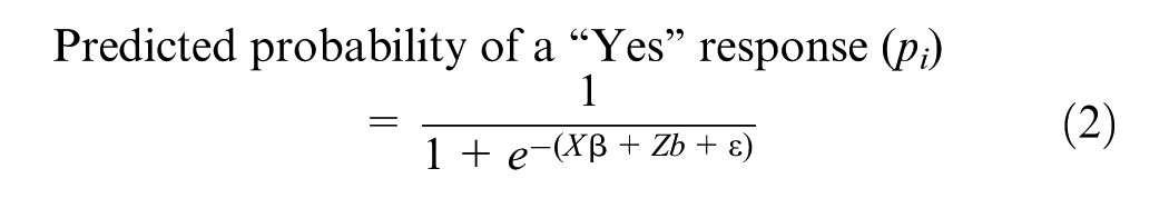
In Equation 1, the linear predictor of the mixed-effect binary logistic regression model was scaled to the response variable using the logit link function, providing the output in the form of log odds. The log odds value can be converted into the probability of a “Yes” response using the inverse of the logistic function, as presented in Equation 2:

\begin{matrix} Predicted probability of a ″ Yes ″ response (p_{i}) \\ = \frac{1}{1 + e^{- (X β + Zb + ε)}} \end{matrix}

(2)

A fixed effects binary logistic regression model was also developed to evaluate the comparative advantage of using a mixed-effects modeling framework. Two models were developed, one mixed effects model and one fixed effects model, in an open-source R Studio statistical software using the lme4 package.

Model Structure

In a regression model, the main effect refers to the direct effect of an independent variable on the dependent variable. The interaction effect refers to the effect of one independent variable on the dependent variable that depends on another independent variable ( 62 ). The interaction effects capture compounding relationships that are not possible with the main effects of the independent variables. Therefore, both the main and interaction effects of driver and road geometric characteristics variables were included in the models. In particular, the interaction effects of order two within driver characteristic variables (e.g., Driving experience×Age), within road geometric characteristics (e.g., R_P×ΔR), and between driver and road geometric characteristics (e.g., Driving experience×ΔR) were included. As R_P, ΔR, and DA were discrete variables. Therefore, these variables were scaled to the range of 0 to 1 using Equation 3 to make them comparable with the driver characteristic variables and achieve model convergence.

Scaled value = \frac{X - Min}{Max - Min}

(3)

where X is the original value of the variable to be scaled, Min is the minimum value of the variable, and Max is the maximum value of the variable.

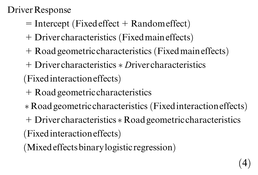
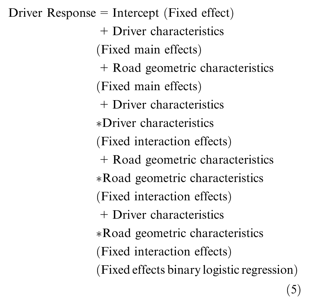
The detailed structures of the two models are presented in Equations 4 and 5. The mixed-effects model (Equation 4) included a fixed intercept, random intercepts for individual drivers and curve combinations, fixed main effects of driver and road geometric characteristics, and fixed interaction effects: (i) within driver characteristics, (ii) within road geometric characteristics, and (iii) between driver and road geometric characteristics. The fixed-effects model (Equation 5) included all the same fixed effects as the mixed-effects model, excluding the random intercepts for individual drivers and curve combinations.

\begin{matrix} Driver Response \\ = Intercept (Fixed effect + Random effect) \\ + Driver characteristics (Fixed main effects) \\ + Road geometric characteristics (Fixed main effects) \\ + Driver characteristics * D river characteristics \\ (Fixed interaction effects) \\ + Road geometric characteristics \\ * Road geometric characteristics (Fixed interaction effects) \\ + Driver characteristics * Road geometric characteristics \\ (Fixed interaction effects) \\ (Mixed effects binary logistic regression) \end{matrix}

(4)

\begin{matrix} Driver Response = Intercept (Fixed effect) \\ + Driver characteristics \\ (Fixed main effects) \\ + Road geometric characteristics \\ (Fixed main effects) \\ + Driver characteristics \\ * Driver characteristics \\ (Fixed interaction effects) \\ + Road geometric characteristics \\ * Road geometric characteristics \\ (Fixed interaction effects) \\ + Driver characteristics \\ * Road geometric characteristics \\ (Fixed interaction effects) \\ (Fixed effects binary logistic regression) \end{matrix}

(5)

Preliminary Analyses

Preliminary analyses were conducted to examine (i) the effects of driver responses on operating speed, and (ii) the effects of curve presentation methods on driver responses, as discussed in the following subsections.

Effects of Driver Responses on Operating Speed

Five curve combinations were selected on a four-lane divided highway (National Highway 52) in Indore, India, to examine the effects of driver responses on operating speed (Table 4). A naturalistic driving experiment was conducted using an instrumented vehicle (i.e., a sedan equipped with a GPS data logger) to record continuous speed profiles and perceptions of the curve combinations. Thirty-four male drivers who held valid driving licenses and had at least two years of driving experience participated in the experiment. A total of 160 speed profiles were obtained after excluding 10 profiles that did not meet free-flow traffic conditions. Drivers typically have a short-term memory span of up to 15 s while driving ( 63 ). Thus, perception data were collected using a questionnaire survey conducted after drivers crossed the consecutive curve combination within 15 s. In this survey, drivers were asked to review the consecutive curve combinations to identify any differences between the horizontal curves and provide their responses in either “Yes” or “No.” A “Yes” response refers to a positive identification of the differences between the curves (i.e., perceived as different), and a “No” response refers to a negative identification of the differences between the curves (i.e., perceived as the same). These responses were then coded into a binary format (i.e., 1 for “Yes” and 0 for “No”). For each curve combination, driver responses were categorized into two groups: No (0) and Yes (1). Drivers’ speed profiles were used to calculate the operating speed (i.e., the 85^th percentile speed, V₈₅) at the midpoint of curves. Subsequently, the change in operating speed (i.e., ΔV₈₅) on each consecutive curve combination was calculated for the driver groups. Table 4 presents the percentage of driver responses and change in operating speed (ΔV₈₅) for the driver groups. It was observed that more than 65% of the driver population positively identified the differences between the curves in the consecutive curve combinations. However, for the 500–100 combination, 46.67% drivers positively identified the difference between the curves. This could be attributable to higher R_P and lower ΔR. The effects of driver responses on ΔV₈₅ were examined using the independent samples t-test. In this test, the mean ΔV₈₅ was compared for the driver groups to identify the significant difference between them. The assumptions of normality (Shapiro–Wilk statistic (response = 0) = 0.912, p-value = 0.479; Shapiro–Wilk statistic (response = 1) = 0.975, p-value = 0.905) and homogeneity of variances (Levene statistic = 0.008, p-value = 0.931) on the data were satisfied at a 5% significance level. Table 4 presents the result summary of the t-test. The difference in ΔV₈₅ for the driver groups had a mean of 4.2 km/h with a standard error of 3.54 km/h. The mean difference in ΔV₈₅ between the driver groups was insignificant at a 5% significance level (t-statistic = 1.186, p-value = 0.27). These preliminary findings suggest no strong evidence of the effects of driver responses on the operating speed.

Table 4.

t-Test Results for Differences in Operating Speed Across Driver Responses

				t-test for differences in ΔV₈₅
Curve combinations (R_P-ΔR) (m)	Driver response category	Driver response percentage (%)	ΔV₈₅ (km/h)	Mean (km/h)	SE (km/h)	t-statistic (p-value)
400–50	No (0)	21.87	16	4.2	3.54	1.186 (0.27)
	Yes (1)	78.13	3
350–100	No (0)	31.25	10
	Yes (1)	68.75	13
500–100	No (0)	53.33	13
	Yes (1)	46.67	6
400–150	No (0)	28.12	23
	Yes (1)	71.88	17
500–250	No (0)	26.67	9
	Yes (1)	73.33	11

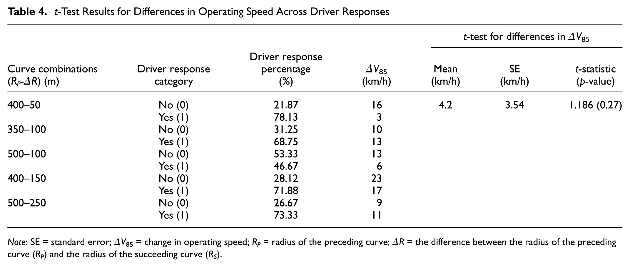
Note: SE = standard error; ΔV₈₅ = change in operating speed; R_P = radius of the preceding curve; ΔR = the difference between the radius of the preceding curve (R_P) and the radius of the succeeding curve (R_S).

Effects of 3D Static and 3D Dynamic Curve Presentation Methods on Driver Responses

Three curve combinations on National Highway 52 were identified and selected to study the effects of presentation methods (i.e., 3D static and 3D dynamic) on driver responses. A naturalistic driving experiment was conducted on the selected curve combinations using an instrumented vehicle (i.e., a sedan equipped with a GPS data logger and a camera), driven at an operating speed of 80–100 km/h, to capture the driver’s perspective of the curves. The driving video was recorded with a high-definition camera placed at a representative driver's view position. Drivers generally start discovering the upcoming curve and accordingly adjust their driving operations (e.g., speed, lane position) from 200 m upstream of the PC ( 64 ). Subsequently, video samples from 200 m to 50 m upstream of the PC were extracted for 3D dynamic curve presentation. A video frame (i.e., image) was also extracted at a 50 m preview distance from the PC for 3D static curve presentation, as shown in Figure 3. The extracted video and image samples of the curve combinations were used to collect perception data using a laboratory-based questionnaire survey. In this survey, a total of 37 drivers (34 males and 3 females) participated and were asked to examine video and image samples of the curve combinations for any differences. The presentation session was divided into two parts. At first, the recorded video clips and then the video frames of the curve combinations were shown to the drivers on a computer screen. A suitable time gap was provided before playing the next set of videos and video frames. Drivers were asked to provide their responses in either “Yes” or “No”. A “Yes” response refers to the positive identification of the differences in curves (i.e., perceived as different), and a “No” response refers to the negative identification of the differences in curves (i.e., perceived as the same). The responses were coded in binary format (i.e., 1 for “Yes” and 0 for “No”). Owing to insufficient representation, data from female drivers were excluded, resulting in a dataset of 34 drivers used for further analysis.

Figure 3.

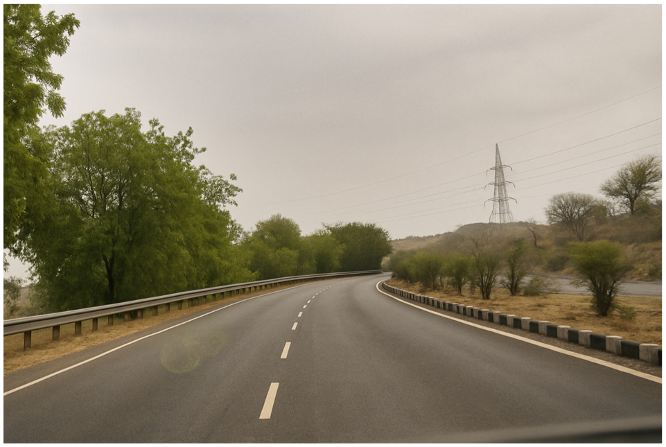
Video frame at 50 m upstream of the curve.

The driver responses were analyzed to test a hypothesis, stated as follows:

H₀ = There is no association between the driver responses and presentation methods, that is, 3D dynamic (field-captured video) and 3D static (field-captured image).

H_a = There is an association between the driver responses and presentation methods, that is, 3D dynamic (field-captured video) and 3D static (field-captured image).

The driver responses were analyzed using the Chi-square test to find associations with the 3D dynamic and 3D static presentation methods. Table 5 presents the distribution of driver responses for the three curve combinations. The Chi-square statistics for the curve combinations (χ² = 0.086, p-value = 0.770; χ² = 0.62, p-value = 0.431; χ² = 0.073, p-value = 0.787) revealed insignificant differences in driver responses between static and dynamic presentation methods at a 5% significance level. These findings suggest that 3D dynamic and 3D static presentation methods are comparable. It also validates the findings of the previous studies (23, 26, 28) and acknowledges the selection of the 3D static presentation method for data collection in the present study, in line with Sil et al. ( 20 ).

Table 5.

Chi-Square Test Results for Differences in Driver Responses Across Presentation Methods

		Number (percentage) of driver responses
Curve combinations (R_P-ΔR) (m)	Driver response category	3D static image, n (%)	3D dynamic video, n (%)	Total, n (%)	Chi-square statistics (χ²)	p-value
400–50	No (0)	8 (53.3)	7 (46.7)	15 (100)	0.086	0.770
	Yes (1)	26 (49.1)	27 (50.90)	53 (100)
	Total	34	34	68
400–150	No (0)	12 (57.1)	9 (42.9)	21 (100)	0.62	0.431
	Yes (1)	22 (46.8)	25 (53.2)	47 (100)
	Total	34	34	68
350–100	No (0)	9 (47.4)	10 (52.6)	19 (100)	0.073	0.787
	Yes (1)	25 (51)	24 (49)	49 (100)
	Total	34	34	68

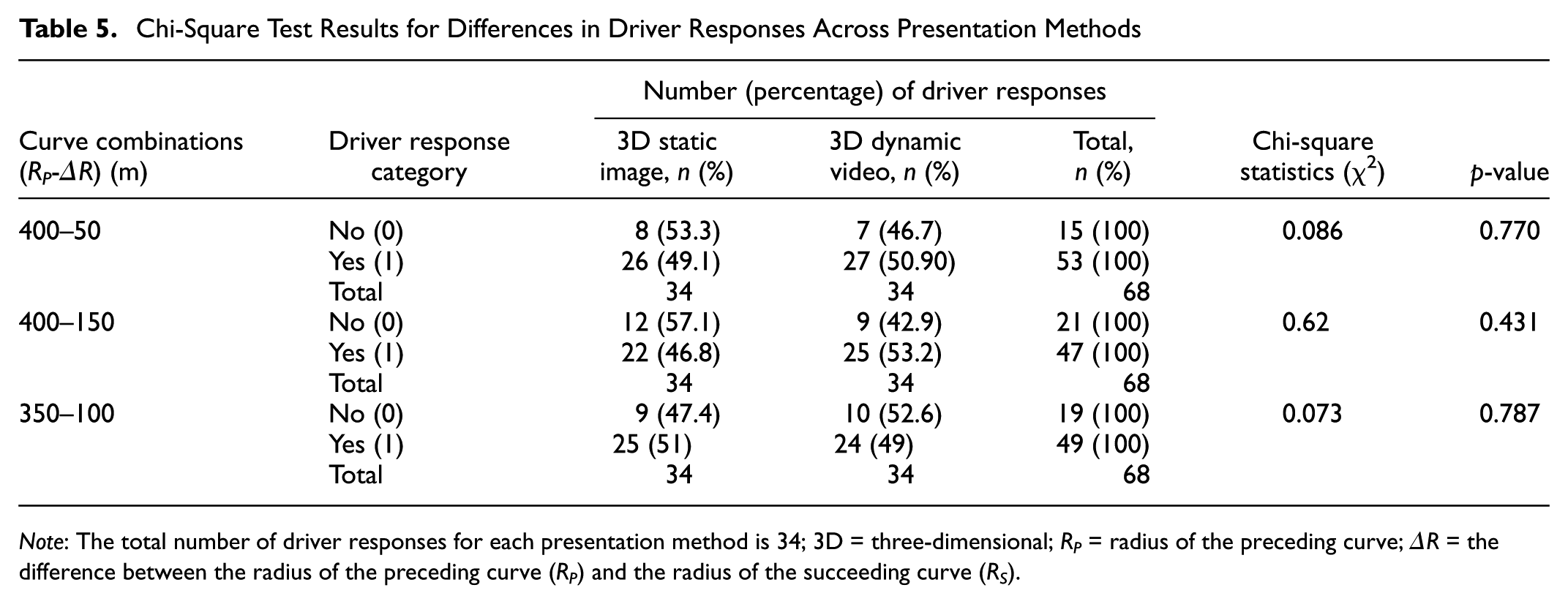
Note: The total number of driver responses for each presentation method is 34; 3D = three-dimensional; R_P = radius of the preceding curve; ΔR = the difference between the radius of the preceding curve (R_P) and the radius of the succeeding curve (R_S).

Analysis

Driver responses were analyzed to quantify the effects of presentation media, driver and road geometric characteristics on consecutive horizontal curve perception. The detailed analytical process is discussed in the following subsections.

Effects of Computer Screen and VR Headset Presentation Media on Driver Responses

Contingency table analysis was used to identify the association between presentation media and driver responses, as both variables were categorical. The effects of a computer screen and a VR headset presentation medium on driver responses were analyzed using a 2×2 contingency table, as presented in Table 6. In total, 1771 “Yes” responses and 1706 “No” responses were recorded from 61 drivers on a computer screen. 1022 “Yes” responses and 916 “No” responses were recorded from 34 drivers on a VR headset. The Chi-square test was used to analyze the contingency table based on the following hypothesis:

Table 6.

Chi-Square Test Results for differences in Driver Responses Across Presentation Media

Presentation medium	Number of drivers	Driver response category	Number of driver responses	Within presentation medium (%)	Chi-square statistics, χ² (p-value)
Computer screen	61	No (0)	1,706	49.10	1.604 (0.204)
		Yes (1)	1,771	50.90
		Total	3,477	100.00
VR headset	34	No (0)	916	47.30
		Yes (1)	1,022	52.70
		Total	1,938	100.00
Total (computer screen and VR headset)	95	No (0)	2,622	48.40
		Yes (1)	2,793	51.60
		Total	5,415	100.00

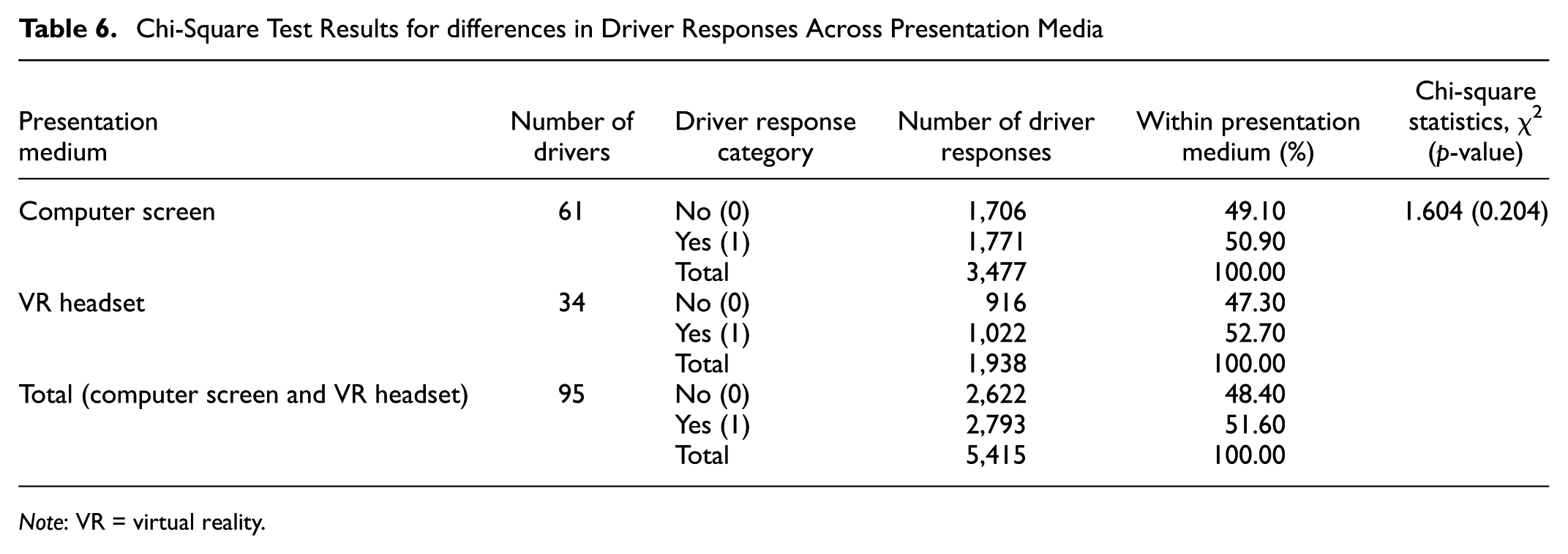
Note: VR = virtual reality.

H_o = There is no association between presentation media and driver responses

H_a = There is an association between presentation media and driver responses

Both presentation media shared a similar proportion of “Yes” responses (50.9% for the computer screen and 52.7% for the VR headset) and “No” responses (49.1% for the computer screen and 47.3% for the VR headset). Table 6 shows that the Chi-square statistics (χ² = 1.604, p-value = 0.204) were consistent in accepting the null hypothesis at a 5% significance level. These results highlight an insignificant relationship between presentation media and driver responses. Therefore, the collected data on both presentation media were comparable and consequently combined for further analysis.

Descriptive Statistics of Driver Responses

Driver responses were classified into driver and road geometric factors and their respective groups, as presented in Figure 4. The responses were also analyzed using the Chi-squared test, as presented in Table 7. Drivers with high driving experience (>10 years) and high annual distance driven (>1,000 km/year) exhibited 2.8% and 3.4% higher “Yes” responses, respectively, compared with drivers with low driving experience (<10 years) and low annual distance driven (<1,000 km/year). These findings suggest that increased driving experience in years and annual distance driven (km) were associated with higher driver perception capabilities of perceiving the differences in horizontal curves. Therefore, driver characteristic factors (Driving experience [year] and Annual distance driven [km]) exhibited significant associations with driver responses (χ² = 4.385, p-value < 0.05; χ² = 4.470, p-value < 0.05). In road geometric factors, “Yes” responses increased when R_P increased from 150 to 200 m, and it decreased when R_P increased from 200 to 400 m. In contrast, “Yes” responses increased when ΔR increased from 50 to 300 m, and DA increased from 30 to 90 degrees. Overall, R_P, ΔR, and DA had significant associations with driver responses (χ² = 21.824, p-value < 0.05; χ² = 555.342, p-value < 0.05; χ² = 22.971, p-value < 0.05). Driver factors such as age, driver type, education, and eyeglasses use, exhibited insignificant relationships with the driver responses (χ²= 1.114, p-value > 0.05; χ² = 0.004, p-value > 0.05; χ² = 0.095, p-value > 0.05; χ² = 0.918, p-value > 0.05). This shows that the driver groups of age, driver type, education, and eyeglasses use had insignificant effects on consecutive horizontal curve perception. Consequently, Driving experience (year), Annual distance driven (km), and road geometric factors (R_P [m], ΔR [m], DA [degree]) were selected as independent variables for driver response model development.

Table 7.

Descriptive Statistics of Driver Responses

		Number (percentage) of driver responses
Groups	Number of drivers	No, n (%)	Yes, n (%)	Total, n (%)	Chi-square statistic ( $χ^{2}$ )
Age (year)
Young (18–30)	51	1,333 (47.7)	1,460 (52.3)	2,793 (100.0)	1.114
Old (>30)	51	1,289 (49.2)	1,333 (50.8)	2,622 (100.0)
Driving experience (year)
Low (≤10)	56	1,446 (49.7)	1,461 (50.3)	2,907 (100.0)	4.385*
High (>10)	46	1,176 (46.9)	1,332 (53.1)	2,508 (100.0)
Annual distance driven (km)
Low (≤1,000)	23	640 (51.0)	614 (49.0)	1254 (100.0)	4.470*
High (>1,000)	75	1,982 (47.6)	2,179 (52.4)	4,161 (100.0)
Driver type
Non-professional	58	1,464 (48.5)	1,557 (51.5)	3,021 (100.0)	0.004
Professional	43	1,158 (48.4)	1,236 (51.6)	2,394 (100.0)
Education
High school	44	1,126 (48.2)	1,211 (51.8)	2,337 (100.0)	0.095
College (graduate/postgraduate)	58	1,496 (48.6)	1,582 (51.4)	3,078 (100.0)
Eyeglasses use
Without eyeglasses	62	1,673 (48.9)	1,747 (51.1)	3,420 (100.0)	0.918
With eyeglasses	36	949 (47.6)	1,046 (52.4)	1,995 (100.0)
R_P (m)
150	na	112 (58.9)	78 (41.1)	190 (100.0)	21.824*
200	na	213 (44.8)	262 (55.2)	475 (100.0)
250	na	386 (50.8)	374 (49.2)	760 (100.0)
300	na	508 (48.6)	537 (51.4)	1,045 (100.0)
350	na	673 (50.6)	657 (49.4)	1,330 (100.0)
400	na	730 (45.2)	885 (54.8)	1,615 (100.0)
ΔR (m)
50	na	1,067 (66.1)	548 (33.9)	1,615 (100.0)	555.342*
100	na	736 (55.3)	594 (44.7)	1,330 (100.0)
150	na	439 (42.0)	606 (58.0)	1,045 (100.0)
200	na	259 (34.1)	501 (65.9)	760 (100.0)
250	na	100 (21.1)	375 (78.9)	475 (100.0)
300	na	21 (11.1)	169 (88.9)	190 (100.0)
DA (degree)
30	na	767 (53.8)	658 (46.2)	1,425 (100.0)	22.971*
60	na	918 (46.0)	1,077 (54.0)	1,995 (100.0)
90	na	937 (47.0)	1,058 (53.0)	1,995 (100.0)

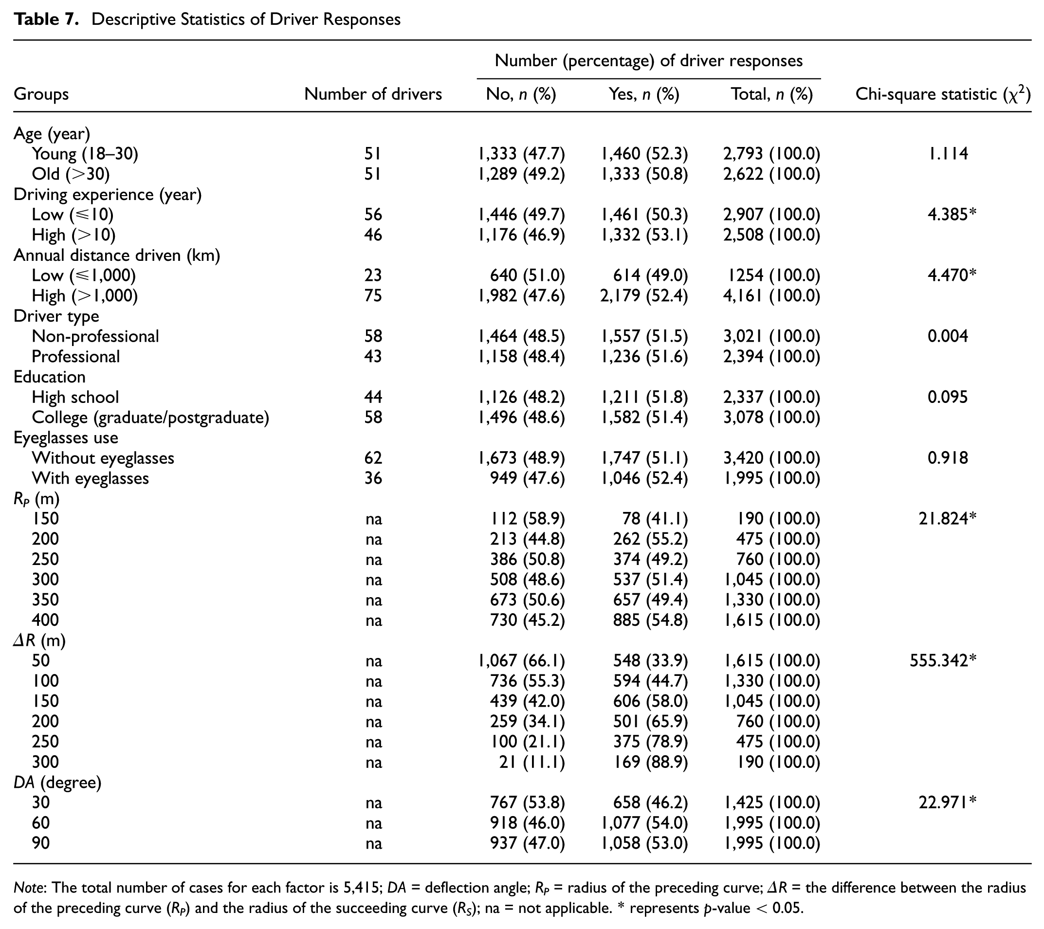
Note: The total number of cases for each factor is 5,415; DA = deflection angle; R_P = radius of the preceding curve; ΔR = the difference between the radius of the preceding curve (R_P) and the radius of the succeeding curve (R_S); na = not applicable. * represents $p$ -value < 0.05.

Figure 4.

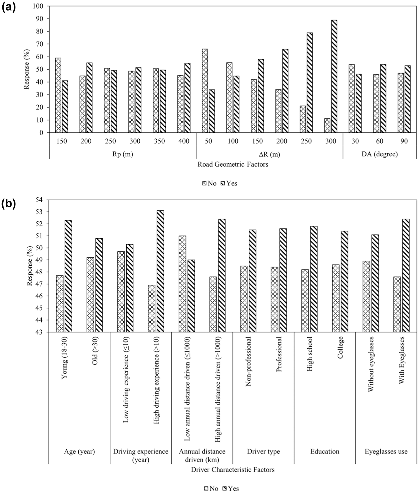
Driver responses across groups of (a) driver characteristic, (b) road geometric factors.

Model Selection

Two driver response models were developed using mixed effects logistic regression (Model 1) and fixed effects logistic regression (Model 2), as presented in Table 8. Table 8 shows the significant predictors, multicollinearity checks, and performance measures of Model 1 and Model 2. The multicollinearity was checked using the variance inflation factor (VIF). The VIF values of predictors for Model 1 (< 4) were lower than for Model 2 (< 7). As a rule of thumb, regression models with VIFs of predictors less than 10 are acceptable ( 65 ). The goodness of fit of the two models was evaluated using Akaike information criteria (AIC) and Bayesian information criteria (BIC). Model 1 had lower AIC (6390 < 6759) and BIC (6469 < 6819) values compared with Model 2. Model 1 had five significant predictors compared with seven in Model 2 at a 5% significance level. Therefore, Model 1 was selected as the final driver response model owing to fewer predictors, lower VIF values of predictors, and better goodness of fit.

Table 8.

Summary of Model Comparison

					Model performance
Model no.	Model type	Input variables	Significant predictors (at 5% significance level)	VIF	AIC	BIC
1	Mixed effects logistic regression	Annual distance driven (km), Driving experience (year), R_P, ΔR, DA, Annual distance driven (km)×R_P,Annual distance driven (km)×ΔR, Annual distance driven (km)×DA,Driving experience (year)×R_P, Driving experience (year)×ΔR, Driving experience (year)×DAΔR×R_P, ΔR×DA, R_P×DA, Annual distance driven (km)×Driving experience (year)	R_P, ΔR,Annual distance driven (km)×ΔR, Annual distance driven (km)×DA,Driving experience (year)×ΔR	< 4	6,390.11	6,469.28
2	Fixed effects logistic regression	Annual distance driven (km), Driving experience (year), R_P, ΔR, DA, Annual distance driven (km)×R_P,Annual distance driven (km)×ΔR, Annual distance driven (km)×DA,Driving experience (year)×R_P, Driving experience (year)×ΔR, Driving experience (year)×DA, ΔR×R_P, ΔR×DA, R_P×DA, Annual distance driven (km)×Driving experience (year)	Annual distance driven (km), Driving experience (year), R_P, ΔR,Annual distance driven (km)×ΔR, Annual distance driven (km)×DA,Driving experience (year)×ΔR	< 7	6,759.20	6,818.58

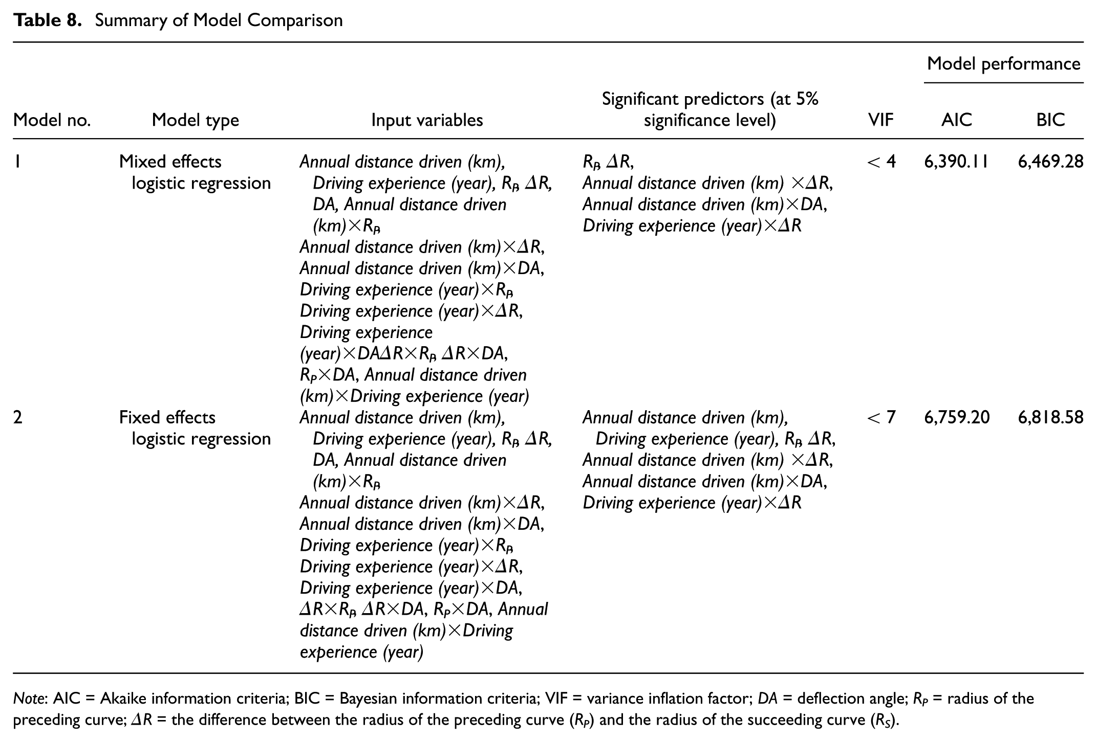
Note: AIC = Akaike information criteria; BIC = Bayesian information criteria; VIF = variance inflation factor; DA = deflection angle; R_P = radius of the preceding curve; ΔR = the difference between the radius of the preceding curve (R_P) and the radius of the succeeding curve (R_S).

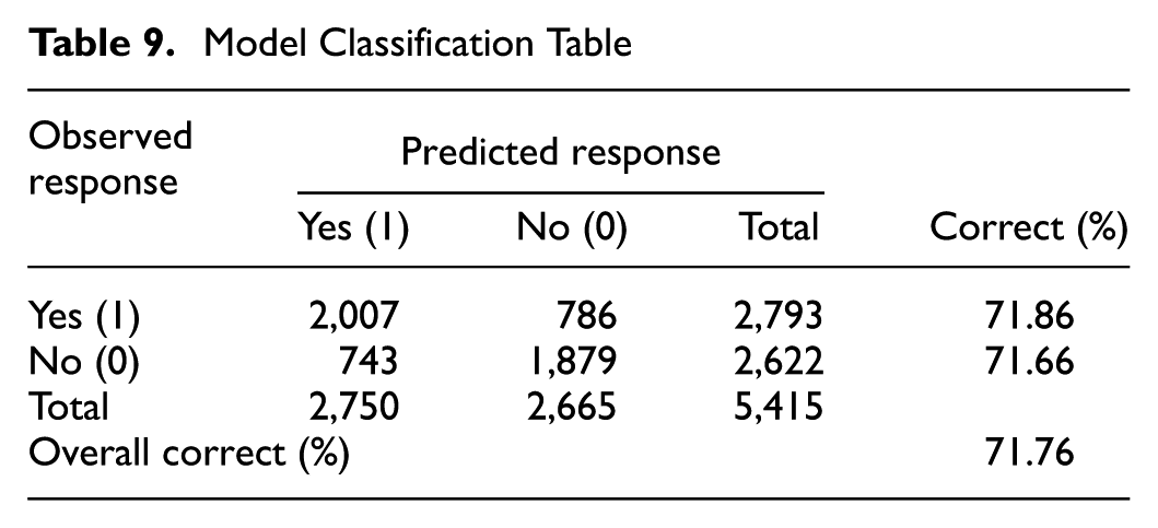
Table 9 presents the classification table of the driver response model, developed using a 0.5 threshold probability ( 20 ). The classification table categorizes the model predictions into four cases: (1) True Positive: when the observed “Yes” response was correctly predicted as “Yes,” (2) False Negative: when the observed “Yes” response was incorrectly predicted as “No,” (3) False Positive: when the observed “No” response was incorrectly predicted as “Yes,” and (4) True Negative: when the observed “No” response was correctly predicted as “No.” Cases 1 and 4 represent correct classifications by the model, while Cases 2 and 3 represent misclassifications. Specifically, the driver response model correctly predicted 2,007 “Yes” responses and 1,879 “No” responses out of a total of 5,415 responses, with accuracy rates of 71.86% and 71.66%, respectively. The overall classification accuracy of the driver response model was 71.76%. Cases 2 and 3 account for the 28.24% misclassification rate of the model.

Table 9.

Model Classification Table

Observed response	Predicted response
	Yes (1)	No (0)	Total	Correct (%)
Yes (1)	2,007	786	2,793	71.86
No (0)	743	1,879	2,622	71.66
Total	2,750	2,665	5,415
Overall correct (%)				71.76

Table 10.

Summary of Driver Response Model

Fixed effects
Predictors	Coefficient	Standard error	z value	p-value
Intercept	0.000	0.287	0.000	1.000
Annual distance driven (km)	0.091	0.292	0.312	0.755
Driving experience (year)	−0.315	0.189	−1.666	0.096
R_P	−1.771	0.321	−5.519	0.000*
ΔR	4.246	0.358	11.847	0.000*
DA	−0.324	0.204	−1.591	0.112
Annual distance driven (km)× R_P	0.481	0.299	1.608	0.108
Annual distance driven (km)×ΔR	−1.822	0.353	−5.155	0.000*
Annual distance driven (km)× DA	0.466	0.189	2.464	0.014*
Driving experience (year)×ΔR	1.533	0.253	6.055	0.000*
Random effects
Clusters	Name	Variance	SD
Drivers	Intercept	0.552	0.743
Curve combinations	Intercept	0.116	0.341
No. of observations	5,415	Clusters: drivers, curve combinations	95, 57

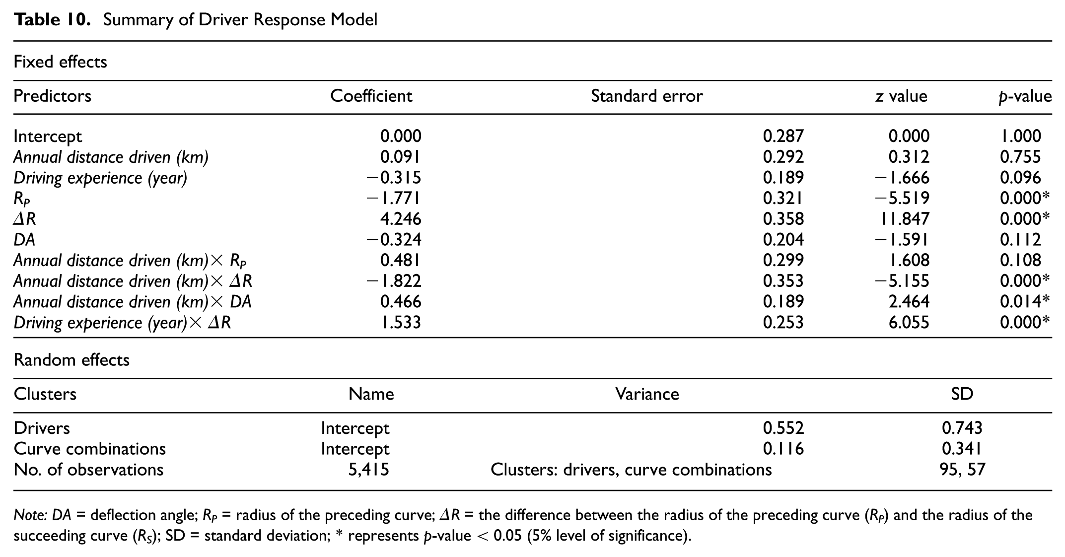
Note: DA = deflection angle; R_P = radius of the preceding curve; ΔR = the difference between the radius of the preceding curve (R_P) and the radius of the succeeding curve (R_S); SD = standard deviation; * represents $p$ -value < 0.05 (5% level of significance).

Prediction misclassifications could be attributable to the three model limitations. First is the absence of random slopes for the independent variables and the lack of interaction effects of order greater than two. These factors might have led to the model's inability to capture the variability in driver responses accurately. Second is the potential non-linear relationships between the variables, which might not have been adequately modeled. Third, the choice of the threshold probability that determines the model classification and misclassification. However, Figure 5 shows that the misclassification rate decreases to 0.5 probability, then increases from 0.5 to 0.9. This finding validates the selection of the 0.5 threshold probability as a suitable option for model classification in this study.

Figure 5.

Effects of threshold probability on model-predicted misclassification.

Results and Discussions

This section discusses the findings of the driver response model and its applications in roadway engineering and policymaking.

Model Findings

R_P, ΔR, Annual distance driven (km)×ΔR, Annual distance driven (km)×DA, Driving experience (year)×ΔR were the significant model predictors at a 5% significance level, as presented in Table 10. The baseline log odds of a “Yes” response (i.e., when predictors are at their reference levels) did not significantly vary at the population level, as indicated by a fixed intercept coefficient of 0.000 and a p-value of 1.000. However, it varied higher across clusters of drivers (SD = 0.743) than across clusters of curve combinations (SD = 0.341). The average marginal effects of predictors on the probability of a “Yes” response (P[“Yes” response]) are presented using scatter plots in Figure 6. The region around the scatter points shows the confidence intervals for the predicted probabilities at a 5% significance level. The detailed discussion on the predictors coefficients and their marginal effects is discussed in the following sections.

Figure 6.

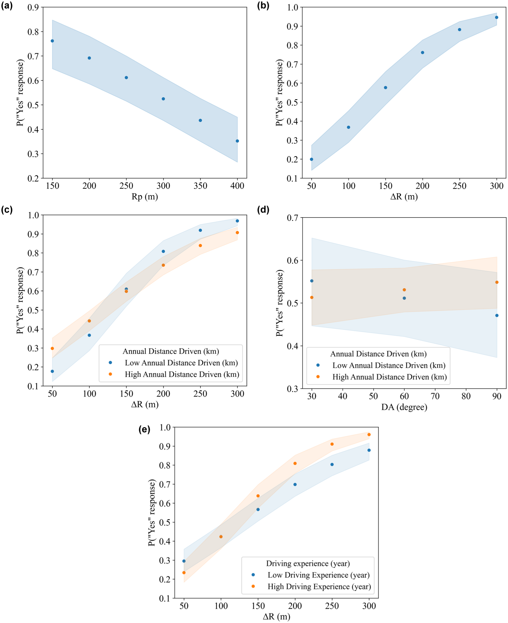
Marginal effects of (a) R_P, (b) ΔR, (c) Annual distance driven (km) × ΔR, (d) Annual distance driven (km) × DA, (e) Driving experience (year) × ΔR on the probability of a “Yes” response.

Single Predictors

RP had a negative coefficient of –1.771 and ΔR had a positive coefficient of 4.246. These coefficients indicate that the log odds of a “Yes” response decrease with R_P and increase with ΔR. In other words, drivers were more likely to perceive differences in horizontal curves with lower radii of preceding curves and higher differences in the radii of preceding and succeeding curves. Figure 6a, and b, shows the marginal effects of R_P and ΔR on P(“Yes” response), respectively. The P(“Yes” response) decreased to 2.2 times when R_P increased from 150 to 400 m and increased 4.7 times when ΔR increased from 50 to 300 m. Further, P(“Yes” response) fell below approximately 0.5 when R_P was greater than 300 m and ΔR was less than 150 m.

Interaction Predictors

Annual distance driven (km) and ΔR had a negative interaction effect on log odds of “Yes” response, with a coefficient of -1.822. Figure 6c shows the marginal effects of ΔR on P(“Yes” response) with respect to Annual distance driven (km). The P(“Yes” response) was lower for drivers with high annual distance driven (>1,000 km) than for drivers with low annual distance driven (≤ 1,000 km) when ΔR ranged from 150 to 300 m, being 0.98 times lower at 150 m and 0.94 times lower at 300 m. It is interesting to observe that P(“Yes” response) for drivers with high annual distance driven (>1,000 km) was decreasing at higher ΔR. Previous studies revealed that experienced drivers often possess low-risk perception and cognitive load for driving tasks owing to their familiarity with similar road geometry conditions (39, 42). As a result, drivers with high annual distance driven (>1,000 km) might have underestimated the differences in horizontal curves. It is to be noted that the P(“Yes” response) was higher for drivers with high annual distance driven (>1,000 km) than for drivers with low annual distance driven (≤ 1,000 km) when ΔR was between 50 and 150 m.

Annual distance driven (km) and DA had positive interaction effects on log odds of a “Yes” response with a coefficient of 0.466. Figure 6d shows the marginal effects of DA on the P(“Yes” response) with respect to Annual distance driven (km). The P(“Yes” response) was higher for drivers with high annual distance driven (>1,000 km) than for drivers with low annual distance driven (≤ 1,000 km) when DA ranged from 60 to 90 degrees, being 1.04 times higher at 60 degrees and 1.16 times higher at 90 degrees. These findings suggest the negative effects of DA on the P(“Yes” response) change to positive with drivers with high annual distance driven (>1,000 km). The higher confidence intervals could be attributed to insignificant main effects of Annual distance driven (km) and DA on log odds of a “Yes” response.

Driving experience (year) and ΔR had positive interaction effects on the log odds of a “Yes” response, with a coefficient of 1.533. Figure 6e shows the marginal effects of ΔR on the P(“Yes” response) with respect to Driving experience (year). The P(“Yes” response) was higher for high-experience drivers (>10 years) than for low-experience drivers (≤ 10 years) when ΔR ranged from 150 to 300 m, being 1.13 times higher when ΔR was 150 m and 1.09 times higher when ΔR was 300 m. Thus, high-experience drivers (> 10 years) perceived the differences in horizontal curves better than the less experienced drivers (≤ 10 years) when ΔR was between 100 and 300 m. In contrast, the P(“Yes” response) was higher for low-experience drivers (< 10 years) than for high-experience drivers (> 10 years) when ΔR was between 50 and 100 m. This could be possible because 44.21% of drivers possessed low experience (≤ 10 years) and higher education (graduate/postgraduate), indicating more technical knowledge about roads. These findings suggest that a higher ΔR helped the high-experience drivers (> 10 years) to perceive the differences in horizontal curves correctly.

Model Applications

The driver response model can be used for engineering applications and formulation of policy recommendations, as discussed in the following subsections.

Engineering Applications

The driver response model can be used for engineering applications to maintain existing highways and design new highways. The consistency or safety of consecutive horizontal curves on existing highways can be evaluated based on the P(“Yes” response) corresponding to R_P, ΔR, and DA.

In the context of maintaining existing highways, road safety engineers can benefit from the predicted P(“Yes” response) in evaluating the consistency or safety of consecutive horizontal curves and providing necessary remedial measures. Engineers can categorize the curve combinations on a safety scale based on the targeted value of P(“Yes” response) (e.g., 0.50). For example, the P(“Yes” response) for curve combinations with R_P between 300 and 400 m and ΔR between 50 and 150 m was less than 0.5 (see Figure 6, a and b). These curve combinations would be rated unsafe for a P(“Yes” response) of 0.5. Similarly, the consistency or safety of other curve combinations based on R_P and ΔR can be evaluated. The same process can be adopted for curve combinations to achieve any other desired threshold of P(“Yes” response). The identified unsafe curve combinations, if treated suitably with speed calming measures, such as advanced curve warning signs (e.g., curve direction), speed warning signs (speed limit), delineation measures (e.g., chevron signs), perceptual measures (e.g., rumble strips), would assist drivers in safe maneuvering across curve combinations ( 66 ). Prior studies reported a decrease in ROR crashes following the installation of such remedial measures ( 67 – 70 ). These measures are effective in controlling vehicle speeds. The reduced vehicular speeds provide drivers with additional time to perceive and respond to upcoming curves. Furthermore, it was reported that speed warning signs and perceptual measures could be more effective in reducing speeds than advanced curve warning signs and delineation measures (67, 69). For instance, engineers can utilize speed warning signs, including in-vehicle speed warning systems and perceptual measures, for curve combinations with the P(“Yes” response) below 0.25 (ΔR = 50 m) (see Figure 6, b, c, and e). The advanced curve warning signs and delineation measures can be utilized for curve combinations with the P(“Yes” response) between 0.25 and 0.5 (300 m < R_P < 400 m, 50 < ΔR < 150 m) (see Figure 6, a–c and e). As recommended by Montella et al. ( 67 ), combinations of speed calming measures could be more effective in assisting a larger driver population in identifying the curve geometry compared with individual measures. Therefore, engineers can use these remedial measures individually or in combination, depending on the targeted threshold of P(“Yes” response). The findings of the driver response model would be instrumental as input for evaluating the consistency or safety of curve combinations and treating them with low-cost speed calming measures.

The findings of the driver response model can also be used to design consecutive horizontal curves of new highways. Engineers can choose the suitable values of geometric features (i.e., R_P, ΔR, and DA) for a targeted value of P(“Yes” response). For example, if the P(“Yes” response) greater than 0.5 is to be achieved, then ΔR should be between 150 and 300 m, R_P should be between 150 and 300 m, and DA should be between 30 and 90 degrees (see Figure 6, a, b, d). Similarly, consecutive curves with other combinations of ΔR, R_P, and DA can be designed for any other targeted value of P(“Yes” response). This process will allow engineers to adopt a customized approach for designing consecutive horizontal curves based on the P(“Yes” response).

Policy Implications

In addition to the road geometric factors, driver characteristic factors (Driving experience [year] and Annual distance driven [km]) exhibited significant effects on the P(“Yes” response). Based on the model coefficients of Annual distance driven (km)×ΔR, Annual distance driven (km)×DA, and Driving experience (year)×ΔR, a set of policy-level interventions and recommendations is discussed below. These specific policy-level considerations can be instrumental in developing driver-oriented geometric design, thereby improving overall road safety.

The model findings revealed that the effects of ΔR and DA on P(“Yes” response) were influenced by driving experience and annual distance driven factors (see Figure 6). The P(“Yes” response) was lower for drivers with low annual distance driven (≤ 1,000 km) than for drivers with high annual distance driven (> 1,000 km) when ΔR was between 50 and 150 m and DA was between 60 and 90 degrees (see Figure 6, c and d). This was also true for low-experience drivers (≤ 10 years) when ΔR was greater than 100 m (see Figure 6e). Previous studies have reported that reduced cognitive impulsiveness in less experienced drivers may impair rational decision-making, while highly skilled and experienced drivers tend to maintain more stable speed control and lateral positioning (41,71). Drivers with high annual distance driven (> 1,000 km) were found with lower P(“Yes” response) when ΔR was between 150 and 300 m (see Figure 6c). This highlights the underestimation behavior of experienced drivers owing to their familiarity with similar road geometric conditions. Thus, the driver response model findings can benefit in identifying vulnerable driver groups based on Driving experience (year) and Annual distance driven (km) that did not conform to certain geometric combinations. Consequently, it highlights the need to educate and train the vulnerable driver groups to adapt to the identified geometric combinations.

Drivers with low annual distance driven (≤ 1,000 km) generally lack advanced driving techniques, hazard perception, and situational awareness. These skills could be inculcated into such drivers through sustained education and training programs ( 42 ). Moreover, supervised driving training can further provide a structured approach whereby drivers with low annual distance driven (≤ 1,000 km) can operate a vehicle under the guidance and supervision of an experienced driver, allowing them to build practical skills in real-world conditions gradually. Therefore, policies should be developed for providing a minimum duration of driving education and supervised driving to drivers with low annual distance driven (≤ 1,000 km) to gain sufficient driving knowledge and practical driving experience. Drivers with high annual distance driven (> 1,000 km) should also undergo periodic training through refresher courses or workshops on risk awareness. During these sessions, they can be evaluated on their risk estimation, confidence, and potential complacency using situational tasks.

These policies can be further implemented to improve licensing laws and procedures in developing countries like India. In this study, 41.05% of the drivers were young (age ≤ 30 years) with low driving experience (≤ 10 years). Young drivers who received their licenses at an early age (around 18 years) were reported to exhibit high crash risks and crash rates during the first few months of a fully privileged license ( 72 ). Thus, newly licensed drivers have high chances of low driving skills and experience in perceiving the differences in horizontal curves. Periodic license renewal can provide a platform for reducing overall crash risks on consecutive horizontal curves. Graduated driver licensing (GDL) can also be effective for drivers with low experience (≤ 10 years) to learn driving skills. GDL is a phased approach to licensing that is successfully implemented and has reduced crashes in developed countries ( 73 ). GDL is not currently implemented in India. Therefore, policies based on GDL can reduce crash risks, particularly for younger and novice drivers with low experience.

Insurance companies consider experienced drivers as low-risk drivers and are more likely to offer them a lower premium. In this study, drivers with high experience (> 10 years) and high annual distance driven (> 1,000 km) had higher P(“Yes” response). This was true for drivers with more than 10 years of experience when ΔR was between 100 and 300 m. Similarly, for drivers who drove more than 1,000 km annually, the effect was observed when ΔR was between 50 and 150 m and the DA was 30 degrees. Therefore, drivers with high experience (> 10 years) and high annual distance driven (> 1,000 km) could be identified as low-risk drivers. Therefore, the study findings could facilitate insurance companies to reframe motor insurance policies based on the driving experience of the vehicle owner.

Conclusions

This study has examined the combined effects of driver and road geometric characteristics on consecutive horizontal curve perception. The preliminary analyses revealed no clear evidence of the effects of driver responses on operating speeds along consecutive horizontal curves. Also, the presentation methods of simulated curve models (i.e., 3D static and 3D dynamic) were statistically comparable. The comparative analysis between the two presentation methods validates the findings of prior studies and supports the 3D static presentation method used in this study. Among the two presentation methods, either method can be suitable for studying horizontal curve perception in a simulated environment. However, the 3D static curve presentation method offers more simplicity in the experimental setup for comparing simulated curve models. Driver responses collected on the computer screen and VR headset were comparable, indicating their advantages as low-cost presentation media over driving simulators in simulated studies on horizontal curve perception. Driver responses revealed insignificant variations across driver groups of age, driver type, education, and eyeglasses use. This finding aligns with the findings of Bidulka et al. ( 23 ), who observed insignificant effects of driver characteristics on curve sharpness perception. The authors concluded that erroneous perception is a universal phenomenon experienced by all driver categories.

The driver response model predicted correct responses with an accuracy of 71.76% at a 0.5 threshold probability. ΔR, R_P, Annual distance driven (km)×ΔR, Annual distance driven (km)×DA, and Driving experience (year)×ΔR were the significant model predictors. The main effects of ΔR and R_P revealed that drivers were able to perceive consecutive curve combinations with lower R_P and higher ΔR. Therefore, such consecutive curve combinations would be safer for drivers. However, no main effects of DA were found. This finding was in line with Sil et al. ( 20 ) about the insignificant effects of deflection angle on distinguishing consecutive horizontal curves. The driver response model can be a valuable tool for engineers to optimize existing highways and design new highways by selecting the appropriate targeted P(“Yes” response). The existing highways can be identified as perceptually inconsistent or unsafe and recommended for treatments (e.g., speed signage and chevron signs). Drivers with low annual distance driven (≤ 1,000 km) had lower P(“Yes” response) as compared with drivers with high annual distance driven (> 1,000 km) when ΔR was between 50 and 150 m, and DA was between 60 and 90 degrees. This was also true for low-experience drivers (≤ 10 years) when ΔR was between 100 and 300 m. Interestingly, the P(“Yes” response) were higher for drivers with low annual distance driven (≤ 1,000 km) than for drivers with high annual distance driven (> 1,000 km) when ΔR ranged from 150 to 300 m. This was also true for low-experience drivers (≤ 10 years) when ΔR was between 50 and 100 m compared with high-experience drivers (> 10 years). These findings highlight the benefits of the driver response model in identifying vulnerable driver groups based on experience who may struggle with certain consecutive curve combinations. Further, the findings highlight the need to educate and train vulnerable driver groups to improve their driving skills. The model’s insights can assist policymakers in developing guidelines for policies such as driving education, supervised driving, and GDL to promote continuous safety awareness and training of drivers throughout their careers.

It is noteworthy to look into the following study limitations and future scopes, which could be the reference for further research in this area.

i Vertical curves also affect the driver's line of sight and visual assessment of horizontal curves. Future studies following a similar methodology to this study can explicitly examine the effects of superimposed 3D alignment in hilly and rolling terrain on consecutive horizontal curve perception. The extension of this study to two-lane highways could also provide more insights into ROR crashes.

ii In this study, the simulated curve models (i.e., 3D static images) were representative of a passenger car moving at a speed of 100 km/h on the inner lane 50 m before PC. Future studies can further explore the effects of operating speed on driver responses using dynamic presentation methods (e.g., driving simulator) to gain a comprehensive understanding of road safety on consecutive horizontal curves.

iii The preliminary analysis of the effects of drivers’ responses on operating speed was conducted with five existing consecutive curve combinations. This was attributable to significant challenges in a field-based study, particularly in selecting representative sites and managing the associated logistical complexities. A further study following the same methodology can be performed to get a deeper understanding and conclusive findings.

iv Representation of female drivers on Indian highways is significantly low (i.e., 6.28%) compared with the male drivers owing to various factors prevalent in developing nations, such as lack of learned drivers, low driving confidence on high-speed roadways, accident fear, social and cultural issues, security concerns, and limited availability of driving training programs designed for women. Subsequently, it affects the low rates of female drivers fatally involved in crashes on Indian Highways. Owing to the participation of an insufficient number of female drivers (only three), this study explicitly used male drivers as its participants. Additional research with both male and female drivers would offer a complete understanding of consecutive horizontal curve perception from a global perspective.

v A comprehensive study examining the effects of variation in roadside scenarios, left versus right turning, and day versus night-time driving could be beneficial for the inclusive effects of driver and road geometric characteristics on consecutive horizontal curve perception.

Footnotes

Acknowledgements

The authors would like to thank Professor Avijit Maji, Professor A.K. Maurya, and Professor Suresh Nama for extending their support with a part of the data used in this study.

Correction (December 2025):

This article has been updated; for further details please see the Article Note at the end of the article.

Article Note

The following sentence in the abstract has been corrected: For new designs, combinations with R_P = 150–300 m, ΔR = 150–300 m, and ΔA = 30–90 degrees were identified as perceptually consistent.

The following sentence in the Engineering Applications section has been corrected: For example, if the P(“Yes” response) greater than 0.5 is to be achieved, then ΔR should be between 150 and 300 m, R_P should be between 150 and 300 m, and ΔA should be between 30 and 90 degrees (see Figure 6, a, b, d).

Author Contributions

The authors confirm contribution to the paper as follows: study conception and design: Mohd Atif, Gourab Sil; data collection: Mohd Atif; analysis and interpretation of results: Mohd Atif; draft manuscript preparation: Mohd Atif, Gourab Sil. All authors reviewed the results and approved the final version of the manuscript.

Declaration of Conflicting Interests

The authors declared no potential conflicts of interest with respect to the research, authorship, and/or publication of this article.

Funding

The authors disclosed receipt of the following financial support for the research, authorship, and/or publication of this article: This research is funded by the Indian Institute of Technology Indore and the Indian Institute of Technology Bombay.

ORCID iDs

Mohd Atif

Gourab Sil

References

World Health Organization. Road Traffic Injuries. https://www.who.int/news-room/fact-sheets/detail/road-traffic-injuries. Accessed February 13, 2024.

Indian Roads Congress. IRC 131: Guidelines for Identifying and Treating Blackspots. Indian Roads Congress, New Delhi, India, 2022.

Kristianssen

A. C.

Andersson

Belin

M. Å.

Nilsen

Swedish Vision Zero Policies for Safety–A Comparative Policy Content Analysis. Safety Science, Vol. 103, 2018, pp. 260–269.

World Health Organization. Global Status Report on Road Safety 2015. World Health Organization, Geneva, Switzerland, 2015.

Cejun Liu

Subramanian

Chen

C.-L.

Hanna

Simons

Kahane

Flemons

, et al. Factors Related to Fatal Single-Vehicle Run-Off-Road Crashes. No. HS-811 232. National Highway Traffic Safety Administration, Washington, D.C., 2009.

Bella

Driver Perception Hypothesis: Driving Simulator Study. Transportation Research Part F: Traffic Psychology and Behaviour, Vol. 24, 2014, pp. 183–196.

International Transport Forum. Zero Road Deaths and Serious Injuries. Leading a Paradigm Shift to a Safe System. OECD Publishing, Paris, 2016.

Kim

Muennig

Rosen

Vision Zero: A Toolkit for Road Safety in the Modern Era. Injury Epidemiology, Vol. 4, No. 1, 2017, pp. 1–9.

Tiwari

Mohan

Traffic Safety in India and Vision Zero. In The Vision Zero Handbook: Theory, Technology and Management for a Zero Casualty Policy (K. Edvardsson Björnberg, S. O. Hansson, M. Å. Belin, C. Tingvall, eds.), Springer International Publishing, Cham, 2022, pp. 1–39.

10.

Fagnant

D. J.

Kockelman

Preparing a Nation for Autonomous Vehicles: Opportunities, Barriers and Policy Recommendations. Transportation Research Part A: Policy and Practice, Vol. 77, 2015, pp. 167–181. https://doi.org/10.1016/j.tra.2015.04.003

11.

Habib

Shalkamy

El-Basyouny

Investigating the Effects of Mental Workload on Highway Safety. Transportation Research Record: Journal of the Transportation Research Board, 2019. 2673: 619–629. https://doi.org/10.1177/0361198119846474

12.

De Waard

Brookhuis

K. A.

The Measurement of Drivers’ Mental Workload. Traffic Research Centre VSC, University of Groningen, The Netherlands, 1996.

13.

Gevins

Smith

M. E.

Neurophysiological Measures of Working Memory and Individual Differences in Cognitive Ability and Cognitive Style. Cerebral Cortex, Vol. 10, No. 9, 2000, pp. 829–839.

14.

Brookhuis

K. A.

van Driel

C. J.

Hof

van Arem

Hoedemaeker

Driving with a Congestion Assistant; Mental Workload and Acceptance. Applied Ergonomics, Vol. 40, No. 6, 2009, pp. 1019–1025.

15.

Hakamies-Blomqvist

Compensation in Older Drivers as Reflected in Their Fatal Accidents. Accident Analysis & Prevention, Vol. 26, 1994, pp. 107–112. https://doi.org/10.1016/0001-4575(94)90073-6

16.

Findley

D. J.

Hummer

J. E.

Rasdorf

Zegeer

C. V.

Fowler

T. J.

Modeling the Impact of Spatial Relationships on Horizontal Curve Safety. Accident Analysis & Prevention, Vol. 45, 2012, pp. 296–304.

17.

Kang

Namgung

Fujiwara

Kim

Wang

Analysis of Vehicle Maneuverability and Driving Characteristics on a Curved Road Condition. KSCE Journal of Civil Engineering, Vol. 23, No. 1, 2019, pp. 420–432. https://doi.org/10.1007/s12205-018-1803-y

18.

Lehtonen

Lappi

Summala

Anticipatory Eye Movements When Approaching a Curve on a Rural Road Depend on Working Memory Load. Transportation Research Part F: Traffic Psychology and Behaviour, Vol. 15, No. 3, 2012, pp. 369–377. https://doi.org/10.1016/j.trf.2011.08.007

19.

Hassan

Sarhan

Operational Effects of Drivers’ Misperception of Horizontal Curvature. Journal of Transportation Engineering, Vol. 138, No. 11, 2012, pp. 1314–1320.

20.

Sil

Maji

Majumdar

B. B.

Maurya

A. K.

Drivers’ Ability to Distinguish Consecutive Horizontal Curves. Canadian Journal of Civil Engineering, Vol. 49, 2022, pp. 1518–1531.

21.

Hassan

Easa

S. M.

Effect of Vertical Alignment on Driver Perception of Horizontal Curves. Journal of Transportation Engineering, Vol. 129, No. 4, 2003, pp. 399–407.

22.

Fleiter

J. J.

Lennon

Watson

How Do Other People Influence Your Driving Speed? Exploring the ‘Who’ and the ‘How’ of Social Influences on Speeding from a Qualitative Perspective. Transportation Research Part F: Traffic Psychology and Behaviour, Vol. 13, No. 1, 2010, pp. 49–62. https://doi.org/10.1016/j.trf.2009.10.002

23.

Bidulka

Sayed

Hassan

Influence of Vertical Alignment on Horizontal Curve Perception: Phase I: Examining the Hypothesis. Transportation Research Record: Journal of the Transportation Research Board, 2002. 1796(1): 12–23.

24.

Hassan

Sayed

Bidulka

Influence of Vertical Alignment on Horizontal Curve Perception: Phase II: Modeling Perceived Radius. Transportation Research Record: Journal of the Transportation Research Board, 2002. 1796(1): 24–34.

25.

Fildes

B. N.

Triggs

T. J.

The Effect of Changes in Curve Geometry on Magnitude Estimates of Road-Like Perspective Curvature. Perception & Psychophysics, Vol. 37, No. 3, 1985, pp. 218–224.

26.

Zakowska

Road Curve Evaluation Based on Road View Perception Study. Transportation Research Record: Journal of the Transportation Research Board, 1999. 1689(1): 68–72.

27.

Hasan

Sayed

Hassan

Influence of Vertical Alignment on Horizontal Curve Perception: Effect of Spirals and Position of Vertical Curve. Canadian Journal of Civil Engineering, Vol. 32, 2005, pp. 204–212.

28.

Hassan

Sayed

Use of Computer Animation in Quantifying Driver Perception of Three-Dimensional Road Alignments. Applications of Advanced Technologies in Transportation, 2002, pp. 877–884.

29.

Ben-Bassat

Shinar

Effect of Shoulder Width, Guardrail and Roadway Geometry on Driver Perception and Behavior. Accident Analysis & Prevention, Vol. 43, No. 6, 2011, pp. 2142–2152.

30.

Vos

Farah

Hagenzieker

How Do Dutch Drivers Perceive Horizontal Curves on Freeway Interchanges and Which Cues Influence Their Speed Choice?

IATSS Research, Vol. 45, 2021, pp. 258–266.

31.

Hassan

Easa

S. M.

Modeling of Required Preview Sight Distance. Journal of Transportation Engineering, Vol. 126, 2000, pp. 13–20.

32.

Charlton

S. G.

Starkey

N. J.

Perrone

J. A.

Isler

R. B.

What’s the Risk? A Comparison of Actual and Perceived Driving Risk. Transportation Research Part F: Traffic Psychology and Behaviour, Vol. 25, 2014, pp. 50–64.

33.

Agrawal

Knodler

Fisher

D. L.

Samuel

Virtual Reality Headset Training: Can It Be Used to Improve Young Drivers’ Latent Hazard Anticipation and Mitigation Skills. Transportation Research Record: Journal of the Transportation Research Board, 2018. 2672(33): 20–30.

34.

Cutello

C. A.

Gummerum

Hanoch

Hellier

Evaluating an Intervention to Reduce Risky Driving Behaviors: Taking the Fear Out of Virtual Reality. Risk Analysis, Vol. 41, No. 9, 2021, pp. 1662–1673.

35.

Pai Mangalore

Ebadi

Samuel

Knodler

M. A.

Fisher

D. L.

The Promise of Virtual Reality Headsets: Can They Be Used to Measure Accurately Drivers’ Hazard Anticipation Performance?. Transportation Research Record: Journal of the Transportation Research Board, 2019. 2673(10): 455–464.

36.

Auberlet

J. M.

Rosey

Anceaux

Aubin

Briand

Pacaux

M. P.

Plainchault

The Impact of Perceptual Treatments on Driver’s Behavior: From Driving Simulator Studies to Field Tests—First Results. Accident Analysis & Prevention, Vol. 45, 2012, pp. 91–98.

37.

Bener

Özkan

Lajunen

The Driver Behaviour Questionnaire in Arab Gulf Countries: Qatar and United Arab Emirates. Accident Analysis & Prevention, Vol. 40, 2008, pp. 1411–1417.

38.

Ministry of Road Transport and Highways (MORTH). Road Accidents in India 2022. MORTH Publications, New Delhi, India, 2022.

39.

Borowsky

Shinar

Oron-Gilad

Age, Skill, and Hazard Perception in Driving. Accident Analysis & Prevention, Vol. 42, 2010, pp. 1240–1249.

40.

Lehtonen

Lappi

Koirikivi

Summala

Effect of Driving Experience on Anticipatory Look-Ahead Fixations in Real Curve Driving. Accident Analysis & Prevention, Vol. 70, 2014, pp. 195–208.

41.

Jiang

The Effects of Situational Factors and Impulsiveness on Drivers’ Intentions to Violate Traffic Rules: Difference of Driving Experience. Accident Analysis & Prevention, Vol. 62, 2014, pp. 54–62.

42.

Choudhari

Maji

Socio-Demographic and Experience Factors Affecting Drivers’ Runoff Risk Along Horizontal Curves of Two-Lane Rural Highway. Journal of Safety Research, Vol. 71, 2019, pp. 1–11.

43.

Öz

Özkan

Lajunen

Professional and Non-Professional Drivers’ Stress Reactions and Risky Driving. Transportation Research Part F: Traffic Psychology and Behaviour, Vol. 13, 2010, pp. 32–40.

44.

Goralzik

Vollrath

The Effects of Road, Driver, and Passenger Presence on Drivers’ Choice of Speed: A Driving Simulator Study. Transportation Research Procedia, Vol. 25, 2017, pp. 2061–2075.

45.

J. J.

Park

Kim

Park

Yun

Investigating the Impacts of Road Traffic Conditions and Driver’s Characteristics on Automated Vehicle Takeover Time and Quality Using a Driving Simulator. Journal of Advanced Transportation, Vol. 2021, No. 1, 2021, p. 8859553.

46.

Shaw

F. A.

Greenwood

A. T.

Bae

Corso

G. M.

Rodgers

M. O.

Hunter

M. P.

Effects of Roadway Factors and Demographic Characteristics on Drivers’ Perceived Complexity of Simulated Roadway Videos. Transportation Letters, Vol. 11, No. 10, 2019, pp. 589–598.

47.

Hills

P. J.

Thompson

Pake

J. M.

Detrimental Effects of Carryover of Eye Movement Behaviour on Hazard Perception Accuracy: Effects of Driver Experience, Difficulty of Task, and Hazardousness of Road. Transportation Research Part F: Traffic Psychology and Behaviour, Vol. 58, 2018, pp. 906–916.

48.

Lyu

Cao

Xie

The Effect of Gender, Occupation and Experience on Behavior While Driving on a Freeway Deceleration Lane Based on Field Operational Test Data. Accident Analysis & Prevention, Vol. 121, 2018, pp. 82–93.

49.

Trapsilawati

Priatna

N. U.

Wijayanto

Widyanti

Syafitri

U. D.

Chamidah

Examining Drivers’ Socio-Demographic Variables and Perceptions Towards Sanction Mechanisms on Speeding Behaviour on Highways: Targeting Appropriate Prevention. Journal of Navigation, Vol. 74, 2021, pp. 726–737.

50.

American Association of State Highway Transportation Officials. A Policy on Geometric Design of Highways and Streets. AASHTO, Washington, D.C., 2018.

51.

Horswill

M. S.

Coster

M. E.

The Effect of Vehicle Characteristics on Drivers’ Risk-Taking Behaviour. Ergonomics, Vol. 45, No. 2, 2002, pp. 85–104.

52.

van Gent

Farah

Van Nes

van Arem

A Conceptual Model for Persuasive In-Vehicle Technology to Influence Tactical Level Driver Behaviour. Transportation Research Part F: Traffic Psychology and Behaviour, Vol. 60, 2019, pp. 202–216.

53.

Hjälmdahl

Várhelyi

Speed Regulation by In-Car Active Accelerator Pedal: Effects on Driver Behaviour. Transportation Research Part F: Traffic Psychology and Behaviour, Vol. 7, No. 2, 2004, pp. 77–94.

54.

Liu

Chen

Gao

Impact of Vehicle Type, Tyre Feature and Driving Behaviour on Tyre Wear Under Real-World Driving Conditions. Science of the Total Environment, Vol. 842, 2022, p. 156950.

55.

Yang

Zheng

Yin

Yamabe

Nakano

Analysis of Influence on Driver Behaviour While Using In-Vehicle Traffic Lights with Application of Head-Up Display. IET Intelligent Transport Systems, Vol. 10, No. 5, 2016, pp. 347–353.

56.

McKenna

F. P.

The Human Factor in Driving Accidents an Overview of Approaches and Problems. Ergonomics, Vol. 25, No. 10, 2010, pp. 867–877.

57.

Indian Roads Congress. IRC: SP: 084: Manual of Specifications & Standards for Four-Laning of Highways. The Indian Roads Congress, New Delhi, India, 2019.

58.

Uteng

T. P.

Gender and Mobility in the Developing World. World Bank, Washington, D.C., 2012.

59.

Ministry of Road Transport and Highways (MORTH). Road Transport Yearbook (2019–20). MORTH Publications, New Delhi, India, 2020.

60.

Dupont

Papadimitriou

Martensen

Yannis

Multilevel Analysis in Road Safety Research. Accident Analysis & Prevention, Vol. 60, 2013, pp. 402–411.

61.

Hox

Multilevel Analysis, Techniques and Applications. Lawrence Erlbaum Associates Publishers, London, 2002.

62.

Aguinis

Gottfredson

R. K.

Best-Practice Recommendations for Estimating Interaction Effects Using Moderated Multiple Regression. Journal of Organizational Behavior, Vol. 31, No. 6, 2010, pp. 776–786.

63.

Wang

Chen

Lin

Using Perception of Alignment and Short-Term Memory to Understand Middle-aged Driver’s Driving Speed on Mountainous Highway. In the 5th International Conference on Transportation Information and Safety (ICTIS), Liverpool, UK, July, 2019, pp. 1098–1104.

64.

Choudhari

Maji

Effect of Horizontal Curve Geometry on the Maximum Speed Reduction: A Driving Simulator-Based Study. Transportation in Developing Economies, Vol. 5, 2019, pp. 1–8.

65.

O’brien

R. M.

A Caution Regarding Rules of Thumb for Variance Inflation Factors. Quality & Quantity, Vol. 41, 2007, pp. 673–690.

66.

Indian Roads Congress. IRC 99: 2018: Guidelines for Traffic Calming Measures in Urban and Rural Areas. Indian Roads Congress, New Delhi, India, 2018.

67.

Montella

Galante

Mauriello

Pariota

Low-Cost Measures for Reducing Speeds at Curves on Two-Lane Rural Highways. Transportation Research Record: Journal of the Transportation Research Board, 2015. 2472(1): 142–154.

68.

Khan

Abdel-Rahim

Williams

C. J.

Potential Crash Reduction Benefits of Shoulder Rumble Strips in Two-Lane Rural Highways. Accident Analysis & Prevention, Vol. 75, 2015, pp. 35–42.

69.

Wang

Zheng

Guidance-Oriented Advanced Curve Speed Warning System in a Connected Vehicle Environment. Accident Analysis & Prevention, Vol. 148, 2020, p. 105801.

70.

Zhao

Rong

The Effect of Chevron Alignment Signs on Driver Performance on Horizontal Curves with Different Roadway Geometries. Accident Analysis & Prevention, Vol. 75, 2015, pp. 226–235.

71.

Upahita

D. P.

Wong

Y. D.

Lum

K. M.

Effect of Driving Experience and Driving Inactivity on Young Driver’s Hazard Mitigation Skills. Transportation Research Part F: Traffic Psychology and Behaviour, Vol. 59, 2018, pp. 286–297.

72.

McCartt

A. T.

Shabanova

V. I.

Leaf

W. A.

Driving Experience, Crashes and Traffic Citations of Teenage Beginning Drivers. Accident Analysis & Prevention, Vol. 35, No. 3, 2003, pp. 311–320.

73.

Shell

D. F.

Newman

I. M.

Córdova-Cazar

A. L.

Heese

J. M.

Driver Education and Teen Crashes and Traffic Violations in the First Two Years of Driving in a Graduated Licensing System. Accident Analysis & Prevention, Vol. 82, 2015, pp. 45–52.