
Abstract
Taxi demand prediction is essential for intelligent transportation systems. Accurate prediction results help address the issue of supply–demand imbalances and enable more efficient traffic management. Significant advances have been made in traffic demand prediction, particularly through the use of deep learning models. However, these models heavily rely on a large amount of data. Data scarcity remains a significant challenge because of high acquisition and storage costs, as well as data sparsity in certain locations and times. Thus, this study proposes a novel taxi demand prediction model that leverages the large language model GPT-2 to capture complex spatio-temporal dependencies. By integrating spatial correlations through a graph attention network and incorporating temporal dependencies at multiple scales, the proposed spatio-temporal taxi demand prediction large model (STTDP-LM) is capable of achieving accurate prediction with limited training data. Extensive experiments validate its effectiveness across two districts in Xi’an. Compared to the baseline method, the STTDP-LM reduces the root mean square error (RMSE), mean absolute percentage error (MAPE), and mean absolute error (MAE) by an average of 12.25%, 12.55%, and 18.33%, respectively, across the two districts. When trained with only 1% of the data, the model still shows significant improvement, with average reductions of 33.83%, 34.12%, and 17.03% in the RMSE, MAE, and MAPE, respectively. The prediction accuracy of the model is more prominent in multi-step prediction with a total duration of 60 min. In summary, this study offers a promising solution for taxi demand prediction with limited historical data, providing a valuable insight for real-world applications in intelligent transportation systems.
Keywords
Taxi transportation plays a vital role in intelligent transportation systems, offering accessible and efficient travel options for passengers. However, taxi service struggles with the challenge of supply–demand imbalance, driven by reasons on both sides ( 1 ). On the supply side, drivers often rely on intuition and experience, leading to inefficient searching behaviors. On the demand side, the travel demand of passengers often fluctuates and is random. This imbalance results in higher cruising times, increased fuel consumption, and longer wait time for passengers. Consequently, establishing an accurate and reliable model to predict taxi demand is crucial for mitigating the imbalance, optimizing resource allocation, and improving traffic management ( 2 ).
The primary objective of taxi demand prediction is to forecast the number of taxi requests in a specific area for a future time period using historical demand data. This challenge has attracted considerable research interest. Various prediction methods have been proposed, with traditional studies predominantly relying on empirical statistics and classical machine learning techniques. More recently, deep learning methods, capable of capturing nonlinear spatial and temporal correlations in taxi demand data, have shown significant success ( 3 , 4 ).
Nevertheless, deep learning models typically require substantial amounts of data. The accuracy of deep learning-based approaches generally improves with an increase in the available training data. However, data scarcity remains a critical challenge, particularly in less developed urban areas. In some cases, collecting sufficient historical data is challenging because of high costs and data sparsity in certain locations and times. This limitation makes it difficult to build a comprehensive taxi demand dataset in many regions, hindering the performance of deep learning models ( 5 , 6 ). As a result, it is essential to develop innovative solutions that address both data scarcity and improve the prediction capabilities of prediction models with limited historical demand data.
The rapid development of large language models (LLMs) has significantly expanded their potential applications beyond natural language processing, offering a promising approach to a wide range of spatio-temporal traffic prediction tasks ( 7 , 8 ). LLMs are deep learning models that have been trained on large, high-quality generalized datasets to capture universal patterns across diverse domains. With their powerful few-shot learning capability and proficiency in cross-modality knowledge transfer, they can be adapted to specific tasks in data-scarce scenarios with only a small amount of fine-tuning data. One key reason LLMs can be effectively applied to taxi demand prediction is the structural similarity between time-series demand data and the data on which LLMs are trained ( 5 ). Both data types can be represented as consistent vectors, enabling LLMs to process them using the same model architecture. This commonality allows LLMs to recognize patterns in sequential data, such as taxi demand fluctuations, and predict future trends.
Thus, this study aims to accurately predict taxi demand using LLMs with limited historical data. While research on LLMs in traffic demand prediction is still limited, existing approaches often overlook the road network topology in spatial modeling with LLMs. Specifically, demand in adjacent areas or regions with similar characteristics tends to follow comparable patterns.
To address this, we propose a novel spatio-temporal taxi demand prediction model based on LLMs that integrates the road network topological structure. Firstly, the spatial correlations, including proximity and connectivity between different areas in the road network, are modeled using a graph attention network (GAT). Temporal correlations are modeled at both daily and weekly scales to capture the patterns and trends in taxi demand. Secondly, the powerful Generative Pre-trained Transformer 2 (GPT-2) is employed for the task. A small amount of historical taxi demand data is used to fine-tune this pre-trained model. To make the time-series demand data comprehensible to LLMs, it is transformed into a token embedding format by GPT-2. GPT-2’s inherent reasoning capabilities are then leveraged to uncover complex spatio-temporal dependencies embedded within the tokenized demand data. Finally, to optimize the fine-tuning process and ensure efficient model adaptation, we dynamically adjust the frozen and tunable layers. This approach enhances prediction accuracy with minimal historical data. In summary, this study aims to improve the effectiveness and accuracy of taxi demand prediction, providing a more robust solution for urban transportation management. The main contributions of this study are as follows.
(1) The study proposes an innovative deep learning model that uses LLMs to capture complex spatio-temporal dependencies, enabling accurate taxi demand prediction with minimal historical data.
(2) The study integrates the road network topology into the LLM-based prediction model for spatial correlation modeling using a GAT. Temporal correlations are captured from multiple perspectives, including origin data, daily patterns, and weekly trends.
(3) The fine-tuning process of LLMs adjusts frozen and trainable layers, optimizing the parameters and ensuring high prediction accuracy.
(4) The study conducts experiments on real datasets to evaluate the model’s prediction performance with both large and small amounts of training data. Multi-step experiments are also performed to verify the effectiveness of long-term predictions. The results demonstrate superior performance of the proposed method.
Literature Review
Taxi Demand Prediction
Various advanced technologies have been developed to model spatio-temporal correlations and predict taxi demand. Traditional time-series forecasting methods, such as the autoregressive integrated moving average (ARIMA) and its variants, have been widely employed in the early stages of taxi demand prediction ( 9 ). However, taxi demand data are typically nonlinear, and the linear assumptions of these models limit their prediction accuracy.
To capture nonlinear dependencies in taxi demand data, traditional machine learning techniques such as multilinear regression (MLR) ( 10 ), support vector regression (SVR) ( 11 ), logistic regression, support vector machines (SVMs) ( 12 ), decision trees, hidden Markov models (HMMs) ( 13 ), and back propagation neural networks (BPNNs) ( 14 ) have been explored. While these methods can model some nonlinearities, they struggle to capture deep, long-term patterns and complex relationships in taxi demand. This limitation is especially evident with large-scale, high-dimensional data, requiring more advanced techniques to model both short-term fluctuations and long-term trends.
To overcome these limitations, advanced deep learning techniques have been increasingly employed. These models are effective at capturing complex, nonlinear, and long-term dependencies in time-series data, providing a more powerful framework for taxi demand prediction in dynamic urban environments. For instance, recurrent neural networks (RNNs) ( 15 ) are commonly used for modeling temporal dependencies. Nevertheless, they suffer from gradient vanishing and explosion in long-term predictions. Long short-term memory (LSTM) ( 1 ) networks and gated recurrent units (GRUs) ( 16 ) address these issues, effectively capturing long-term dependencies, with GRUs offering faster training. Moreover, several advanced deep learning approaches, such as attention mechanism-based methods ( 17 , 18 ) and graph neural networks ( 19 ), have been proposed to better capture spatio-temporal dependencies and improve prediction performance.
Traditional methods heavily rely on a large amount of data. For example, Kim et al. ( 10 ) employed a MLR model on NYC taxi data from 2015 to 2017, achieving a root mean square error (RMSE) of 0.1129 and a mean absolute percentage error (MAPE) of 15.04% for single-step prediction. Zhe and Su ( 14 ) proposed a Spark-based optimized BPNN model, reaching a prediction accuracy of 90.2% using 2 years of data (2017–2018) for training and one year (2019) for validation. Liu et al. ( 1 ) applied a modified LSTM framework on NYC taxi data from 2014 and obtained an origin-destination MAPE (OD-MAPE) of 24.93% and an origin MAPE (O-MAPE) of 12.92%. Xu et al. ( 15 ) designed a sequential learning model based on RNNs and mixture density networks, achieving 83% prediction accuracy using NYC taxi data collected between January 2013 and June 2016. Although these models achieved promising results, they heavily rely on large-scale, long-span historical data for training. Data scarcity is a significant challenge in urban sensing applications, particularly in less developed areas with limited or no data collection infrastructure. In many cases, gathering the required data becomes particularly difficult because of high acquisition, storage, and maintenance costs. Moreover, in dynamic environments with constantly changing demand patterns, the lack of comprehensive and up-to-date data makes it even harder to maintain reliable predictions over time. Therefore, accurately predicting taxi demand with limited historical data is essential.
LLMs for Traffic Data Prediction
LLMs have strong learning capabilities, allowing them to learn effectively from a small number of samples. LLMs have recently been employed in traffic prediction. For instance, Huang ( 7 ) used a LLM to process traffic textual information and generate embeddings. These embeddings were combined with historical traffic data. They were then input into traditional spatio-temporal prediction models to explore the potential impact of non-numerical context information, such as special situations or weather, on traffic flow. Guo et al. ( 8 ) proposed a traffic flow prediction model based on LLMs to generate explainable predictions. They designed a structured textual prompt that incorporates multi-modal traffic flow information, facilitating LLMs to capture traffic patterns better. It was the first study to apply LLMs for explainable traffic flow prediction and it demonstrated effective generalization abilities across different traffic flow prediction scenarios without additional training. Ren et al. ( 5 ) proposed a framework named traffic prediction large language model (TPLLM) for traffic prediction based on pre-trained LLMs, to cope with full-sample and few-shot traffic prediction tasks. They designed an embedding module to enable LLMs to understand time-series data and to fuse spatio-temporal features implied within the traffic data. In addition, to reduce training costs and maintain high fine-tuning quality, they applied a cost-effective fine-tuning method, LoRA, to the TPLLM. Their approach effectively supported the development of intelligent transportation systems in areas with limited historical traffic data. Liu et al. ( 20 ) proposed a spatio-temporal LLM for traffic prediction, which defined timesteps at a location as a token and embedded each token with a spatio-temporal embedding layer. Meanwhile, they partially froze the multi-head attention (MHA) to capture global spatio-temporal dependencies between tokens for different traffic prediction tasks. Its framework demonstrated strong performance in both few-shot and zero-shot prediction scenarios. Rong et al. ( 21 ) proposed a lightweight spatio-temporal generative LLM for traffic flow forecasting. Their framework used a spatio-temporal module to capture the spatio-temporal correlations. In addition, they used a parameter transfer strategy to implement the “inference while train” mode, accelerating the training. It not only demonstrated strong prediction performance but also effectively reduced the computational burden of training on large-scale data. De Zarzà et al. ( 22 ) introduced real-time interventions with lightweight LLMs in autonomous driving. By combining a language-and-vision assistant with deep probabilistic reasoning, they improved the system’s real-time responsiveness. Peng et al. ( 23 ) proposed a lane-change LLM that treated the task as a language modeling problem. It predicted lane-change intentions and trajectories, offering explanations to improve interpretability, marking the first use of LLMs for lane-change behavior prediction.
According to the aforementioned literature, LLMs have been widely applied in traffic prediction tasks and have demonstrated strong performance, especially with limited data. However, few studies focus on taxi demand prediction using LLMs. Furthermore, current research on taxi demand prediction using LLMs neglects the adjacency relationships between spatial regions, which are crucial for spatial modeling. As a result, developing a novel LLM-based approach that incorporates road network topology is a significant challenge, requiring solutions for spatial modeling in LLMs and addressing data scarcity.
Methodology
Problem Statement
The purpose of this study is to predict the taxi demand by leveraging historical demand data, which is processed from taxi order records aggregated into specific time intervals. The historical taxi demand is computed by dividing the daily taxi orders into time intervals based on a specified time granularity. For example, when the time granularity is set to 10 min, staring from 7:00 a.m., the first time interval would be from 7:00 to 7:10 a.m., followed by 7:10 to 7:20 a.m., and so on. Since taxi demand is highly correlated across neighboring regions, modeling the spatial dependencies among regions is crucial. The graph structure provides a natural way to represent spatial relationships between regions, and GAT can further capture the dynamic importance of each neighboring region through its attention mechanism.
Definition 1: Traffic network
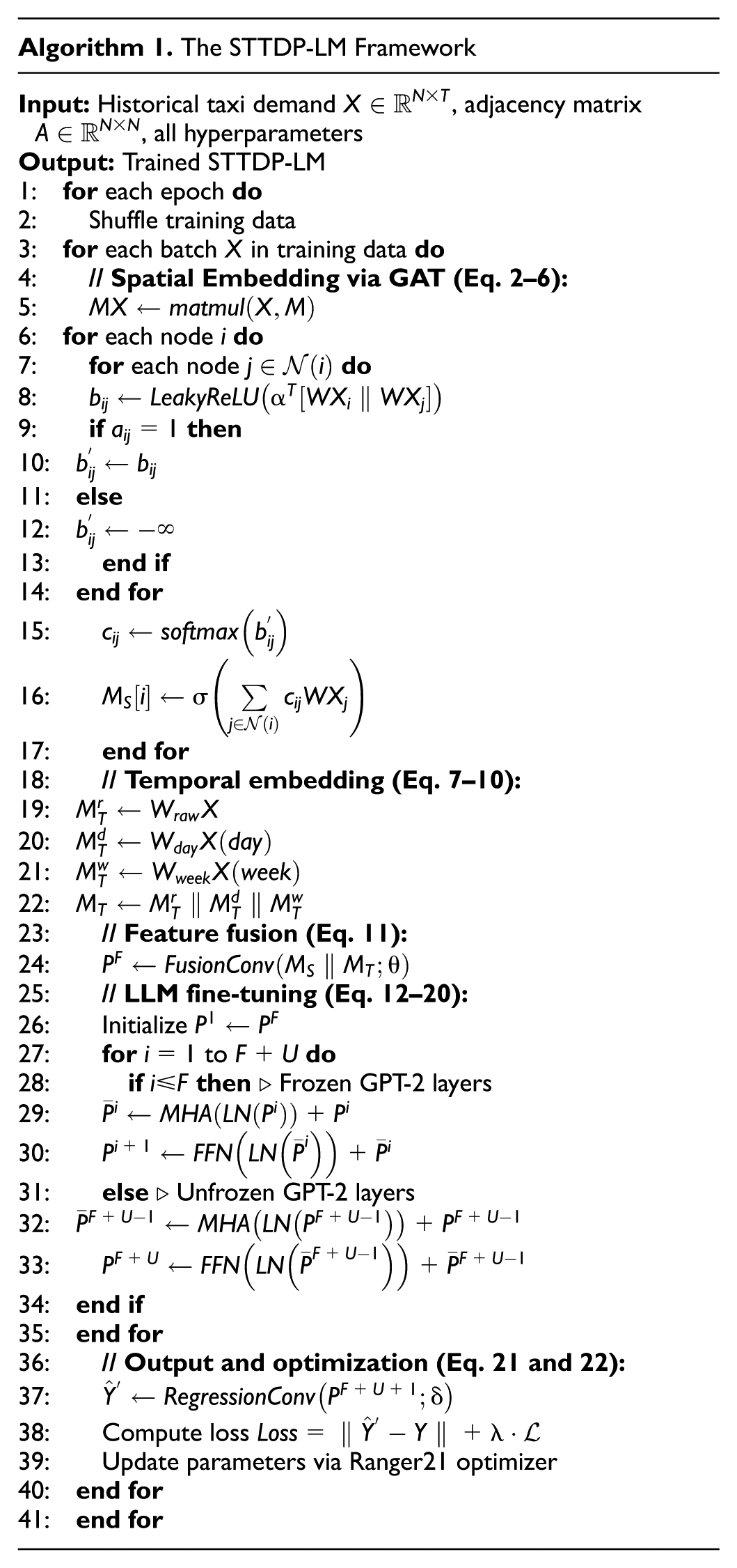
Definition 2: Taxi demand prediction problem. The historical taxi demand data of all grids at the
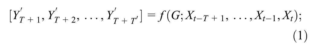
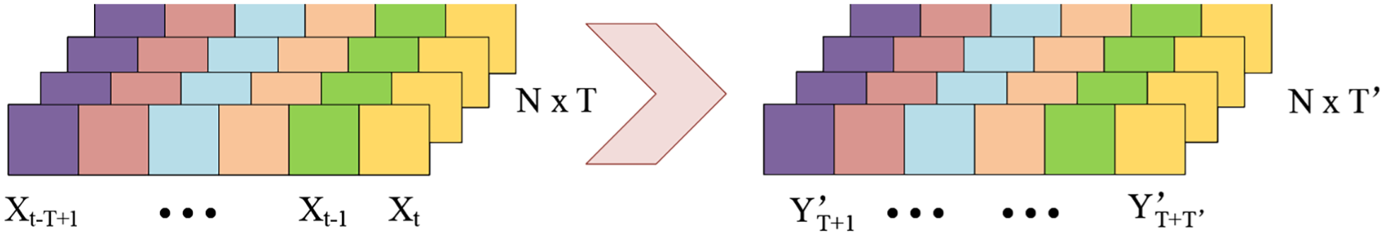
Schematic diagram of the taxi demand prediction problem.
Overall Framework
To accurately predict taxi demand with limited data, we propose a spatio-temporal taxi demand prediction large model (STTDP-LM) through fine-tuning the LLM GPT-2, as illustrated in Figure 2.
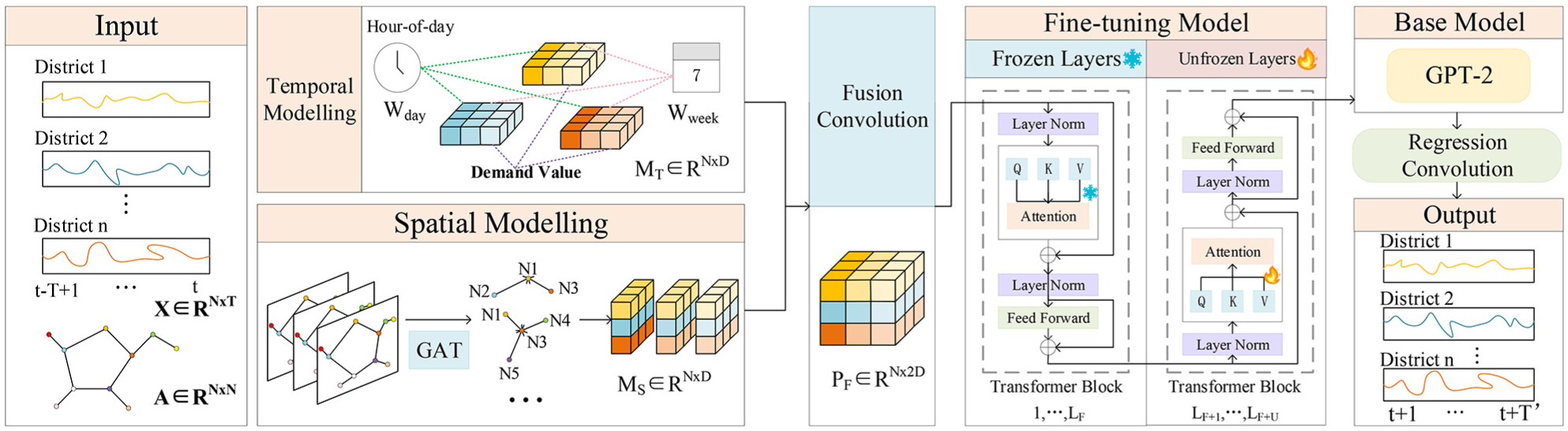
Framework of the proposed spatio-temporal taxi demand prediction large model (STTDP-LM).
The framework processes taxi demand of all nodes over the past
Graph Attention Network for Spatial Modeling
In real-world traffic networks, there exist hidden spatial correlations between different nodes. These spatial correlations primarily stem from road connectivity, which influences how demand in one area might affect surrounding areas. Nodes that are connected through the road network are likely to have more similar demand patterns. Therefore, capturing these spatial correlations is crucial for enhancing the predictive performance of models.
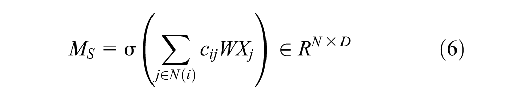
Because of the complex and dynamic nature of traffic networks, graph-based models provide a natural and flexible framework to represent and model these spatial correlations. To better capture the spatial correlations in the demand data between nodes, this study utilizes the GAT for spatial modeling of the node demand data. The GAT allows the model to dynamically assign different attention weights to neighboring nodes based on their importance in predicting demand. This enables the model to incorporate spatial dependencies in a flexible and adaptive manner.
Firstly, the historical demand data

Then, to understand how the nodes interact within the graph and capture the relationship between the demand data of node

After obtaining the attention coefficients, the adjacency matrix is used to perform the masking operation to ensure that attention is only computed between nodes that are connected in the graph (i.e., where there is an edge between them). The coefficients are then normalized using the softmax function. The equations are as follows:


where
Finally, the spatial embedding
Multi-Scale Temporal Modeling
Taxi demand data is influenced by both spatial distribution and temporal variations, such as daily fluctuations and weekly trends. These temporal dynamics are crucial for accurate predictions, as they reflect how demand evolves under different conditions. Therefore, capturing temporal dynamic changes is crucial to improving model accuracy
To model these temporal variations effectively, a linear layer is used to encode the raw input data into separate time embedding at different scales. Embeddings are learned feature representations that map the raw data into fixed-size vectors, capturing underlying patterns and trends over time. In addition to the linear changes in the raw temporal demand data, absolute position encoding is applied to each demand data at “daily” and “weekly” scales. This enables the model to fully capture temporal correlations and patterns across different time intervals. The equations for the multi-time scale embeddings are as follows:


where

Spatio-Temporal Feature Fusion
While both spatial and temporal models extract meaningful features, they each focus on one dimension—spatial or temporal. After spatial modeling and temporal modeling, the extracted features from both domains capture important but distinct aspects of the taxi demand prediction task. Spatial modeling is designed to capture the underlying relationships between different nodes in the traffic network. This modeling provides spatial embeddings that represent how demand is influenced by nearby nodes. However, these spatial embeddings alone are insufficient to fully account for the temporal fluctuations in taxi demand. On the other hand, temporal modeling focuses on capturing the time-varying patterns in taxi demand. By utilizing historical demand data and patterns such as daily fluctuations and weekly trends, temporal modeling generates temporal embeddings. These embeddings reflect how demand changes over time but do not incorporate spatial relationships.
To capture both spatial and temporal dependencies simultaneously, a fusion convolution layer is employed. The fusion convolution layer integrates the spatial and temporal embeddings into a unified representation that can simultaneously account for the interactions between spatial nodes and time-varying demand patterns. It enables the model to learn and represent the complex spatio-temporal relationships about taxi demand. The fusion convolution layer projects the fused feature representation to the required dimensions for further processing by the LLM. The equation for this fusion operation is as follows:

where
LLM Fine-Tuning and Model Prediction
After spatio-temporal feature fusion, the fused vector is input into the fine-tuning model for further tuning. The base model is GPT-2. In the fine-tuning model, the first
In the first


where
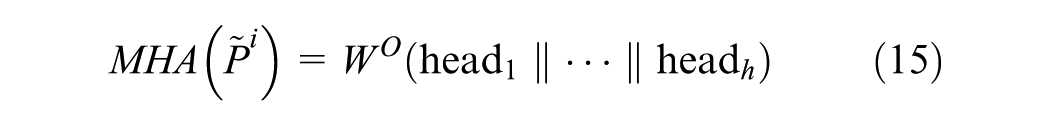
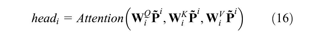
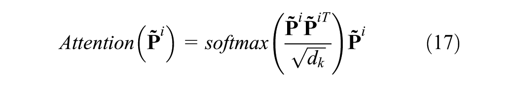
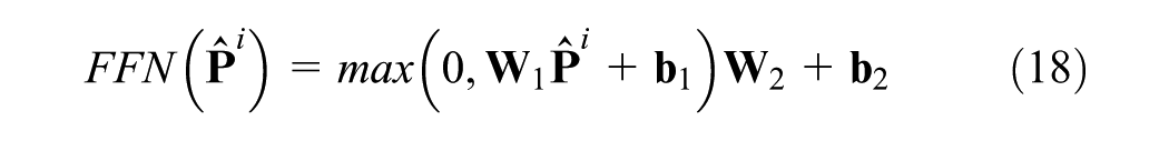
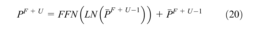
Details of the internal operation of GPT-2 are shown in Equations 14–18, which are designed to further capture the spatio-temporal dependencies within the tensor output from the fusion convolution layer. The core components include LN, MHA, and the FFN. LN is used to stabilize the learning process by normalizing the activations of each layer. The MHA captures long-range temporal and spatial dependencies through a self-attention mechanism that enables each element in the sequence to attend to all previous elements. The FFN performs nonlinear transformations independently at each position, enhancing the model’s expressive capacity and enabling it to learn complex feature interactions:

where
In the final

After fine-tuning the LLM, the regression convolution (RConv) is used to predict the taxi demand for the following

The loss function of the ST-LLM is established as follows:

where
Experiments
Dataset
This study uses taxi trajectory data from Xi’an, covering taxi operations from February 28, 2019, to March 30, 2019. We first converted the coordinate system of the collected trajectory data. Then, we cleaned the data by removing abnormal GPS points and performing map matching using a HMM ( 24 ) to correct GPS drift. After that, we extracted the origin and destination of each trip. We used TransBigData to aggregate the trajectory data with a 10-min time interval. Each trip record was mapped to a predefined 1 km × 1 km spatial grid based on its longitude and latitude. TransBigData is an open-source Python toolkit designed for processing and analyzing spatio-temporal transportation data, such as taxi trajectories, floating car data, and shared bike data. It provides useful tools such as map matching, trajectory cleaning, grid-based spatial division, and origin–destination matrix generation. In addition, the 1-km grid strikes a balance between spatial resolution and computational efficiency. A smaller grid would increase complexity and result in sparse data, while a larger grid would simplify calculations but may not meet the precision requirements for accurate positioning ( 1 , 25 , 26 ).
Figure 3 shows a map of the main urban area of Xi’an before and after grid division. Figure 4 presents the spatial distribution of taxi demand at three time periods on both weekdays and non-working days. In general, the demand hotspots during all three time periods are mostly concentrated in the central area of the map. The color depth of each grid represents the demand level. Darker colors indicate higher demand in that grid. From 07:00 to 08:00, high-demand areas are more concentrated. This suggests that travel patterns during the morning peak are more fixed. Taxi demand mainly appears near residential areas, transport hubs, and commuting routes. On non-working days, the hotspot areas are fewer compared to weekdays. From 12:00 to 13:00, demand is still focused in the central area, but the high-demand zones become more spread out. This may be caused by people going out for lunch or errands, which leads to more scattered activity. From 19:00 to 20:00, the demand distribution is even more dispersed, especially in the central area. This may be related to people engaging in various activities after work.
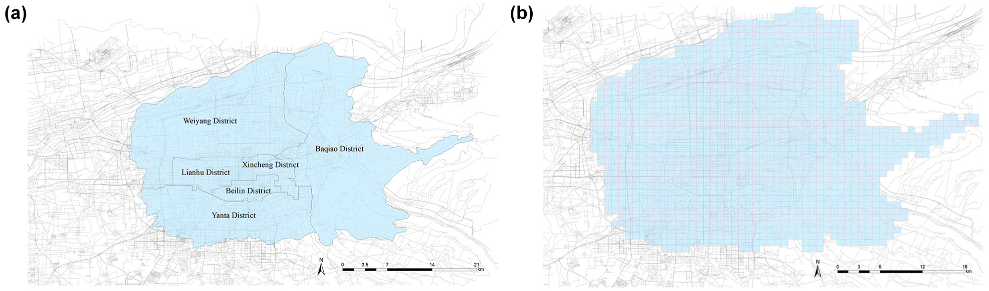
Study area: (a) the main urban area of Xi’an; (b) grid division result.
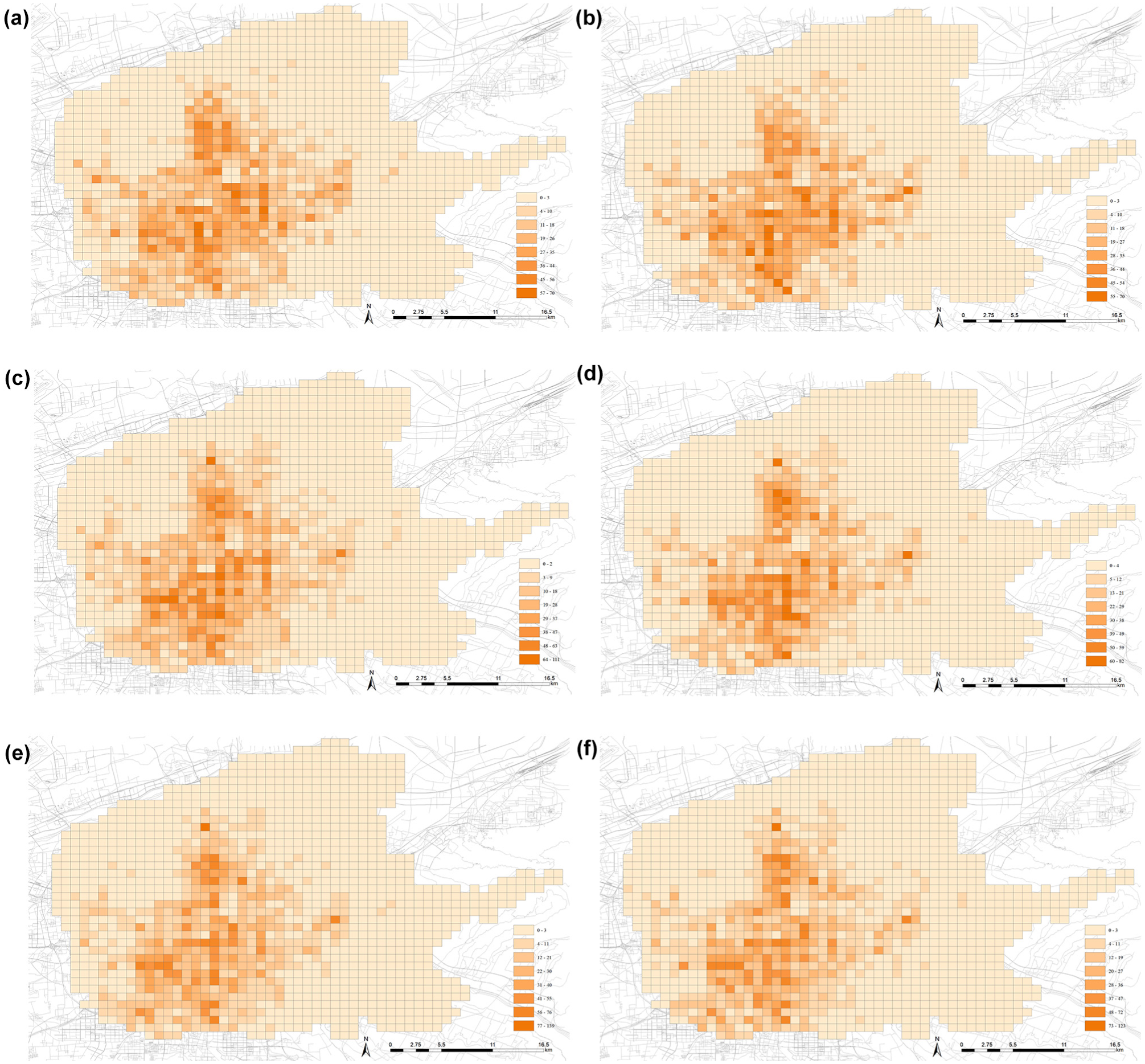
Distribution of taxi demand space in different periods: (a) weekday (07:00–08:00); (b) weekend (07:00–08:00); (c) weekday (12:00–13:00); (d) weekend (12:00–13:00); (e) weekday (19:00–20:00); (f) weekend (19:00–20:00).
Xincheng and Lianhu districts are selected as the primary research areas because of their size and demand density. In the following sections, Xincheng district will be referred to as district 1, and Lianhu district will be referred to as district 2. The total demand for all days in the dataset for districts 1 and 2 is 1,111,164 and 1,183,826, respectively. The average daily demand per grid in each district is 535 and 530, respectively. Taking district 1 as an example, after grid partitioning, there are 67 grids in total. The historical demand values of these 67 grids are fed into the model for training. The model uses the demand values from the past 12 timesteps of each grid to predict the demand values for the next timestep.
Experiment Settings and Evaluation Metric
To evaluate the effectiveness of the proposed STTDP-LM, a series of well-designed experiments are conducted. The baseline methods include the SVR, LSTM, GRU, GAT, graph convolutional network (GCN), and spatial-temporal graph convolutional network (STGCN). To verify the effectiveness of spatio-temporal correlation modeling, two ablation models are designed based on the large model (STTDP-LM-Spatial, STTDP-LM-Temporal). The STTDP-LM-Spatial only utilizes spatial embeddings, without temporal embeddings, while the STTDP-LM-Temporal employs only temporal embeddings. The STTDP-LM-Spatial and STTDP-LM-Temporal methods are based on the proposed approach and are designed for ablation experiments, so they are not part of the baseline methods.
The dataset is divided into training, validation, and test sets with a 6:2:2 ratio. Both the LSTM and GRU models consist of 64 neurons. We set the historical timesteps
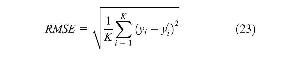
The evaluation criteria include the RMSE, MAPE, and mean absolute error (MAE), which are defined by the following equations. In these equations,


Overall Prediction Performance
We conduct taxi demand prediction experiments using our proposed methods (STTDP-LM, STTDP-LM-Spatial, STTDP-LM-Temporal) along with several baseline models. The STTDP-LM-Spatial and STTDP-LM-Temporal are variations of the STTDP-LM that use only spatial or temporal components, respectively. Baseline methods include traditional models (ARIMA, SVR) and deep learning models (LSTM, GRU, GAT, GCN, STGCN). The overall prediction results for the next timestep in districts 1 and 2 are summarized in Table 1, with detailed results presented in Figure 5. The values are computed for all test observations by comparing the actual and predicted values.
Prediction Results of Traditional Methods (ARIMA, SVR), Deep Learning Methods (LSTM, GRU, GAT, GCN, STGCN), their Average, and the STTDP-LM
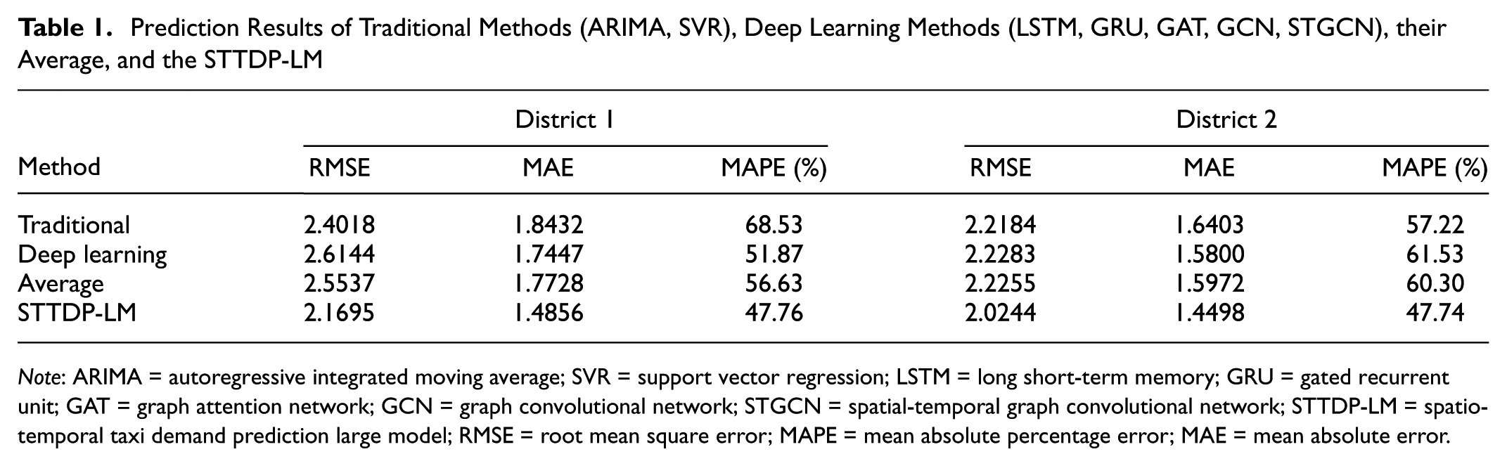
Note: ARIMA = autoregressive integrated moving average; SVR = support vector regression; LSTM = long short-term memory; GRU = gated recurrent unit; GAT = graph attention network; GCN = graph convolutional network; STGCN = spatial-temporal graph convolutional network; STTDP-LM = spatio-temporal taxi demand prediction large model; RMSE = root mean square error; MAPE = mean absolute percentage error; MAE = mean absolute error.
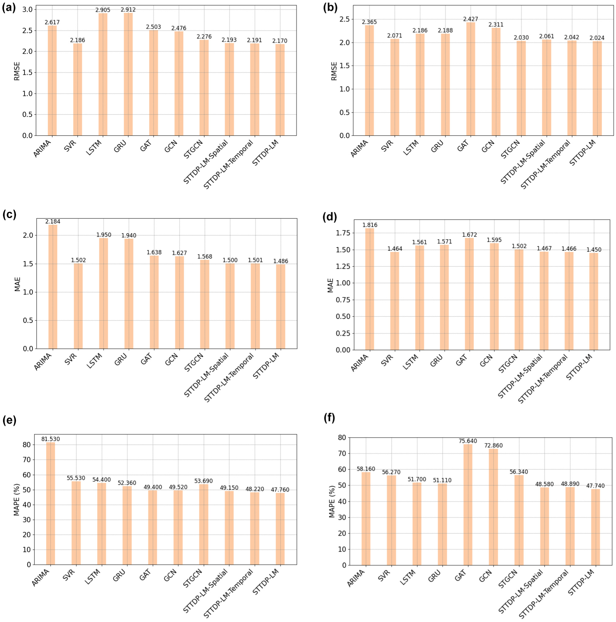
Comparison of prediction results for districts 1 and 2 using different methods: (a) root mean square error (RMSE) results of district 1; (b) RMSE results of district 2; (c) mean absolute error (MAE) results of district 1; (d) MAE results of district 2; (e) mean absolute percentage error (MAPE) results of district 1; (f) MAPE results of district 2.
According to Table 1, the STTDP-LM outperforms the baseline methods across the three evaluation metrics in both districts. Specifically, in district 1, the RMSE, MAE, and MAPE are 2.1695, 1.4856, and 47.76%, respectively. The average RMSE, MAE, and MAPE values of all compared methods are 2.5537, 1.7728, and 56.63%, respectively. The STTDP-LM demonstrates an overall reduction of 15.04%, 16.20%, and 15.66% in these metrics compared to the average values of all baseline methods. In district 2, the RMSE, MAE, and MAPE are 2.0244, 1.4498, and 47.74%, respectively, with the average values for baseline methods being 2.2255, 1.5972, and 60.30%, respectively. The STTDP-LM achieves an overall reduction of 9.04%, 9.23%, and 20.83% in these three metrics. The results of the STTDP-LM-Spatial and STTDP-LM-Temporal indicate that combining spatial and temporal embeddings in the STTDP-LM leads to superior prediction performance. These results demonstrate that the STTDP-LM can accurately predict future demand using only 2 h of historical data. This capability makes it highly applicable to ride-hailing or taxi dispatching systems. By leveraging short-term historical data for high-accuracy forecasting, the model enables more efficient vehicle allocation, reduces passenger wait times, and minimizes idle driving rates.
Figure 6 shows the effectiveness of incorporating spatial and temporal modeling into the LLM. As depicted, the model that includes both components (STTDP-LM) consistently outperforms its variants, the STTDP-LM-Spatial and STTDP-LM-Temporal. Specifically, when both spatial and temporal modeling are incorporated into GPT-2, the RMSE, MAE, and MAPE values are the lowest, indicating better prediction accuracy. In contrast, using only one of the components results in slightly lower performance. This highlights that simultaneously accounting for both spatial and temporal modeling enhances prediction accuracy.
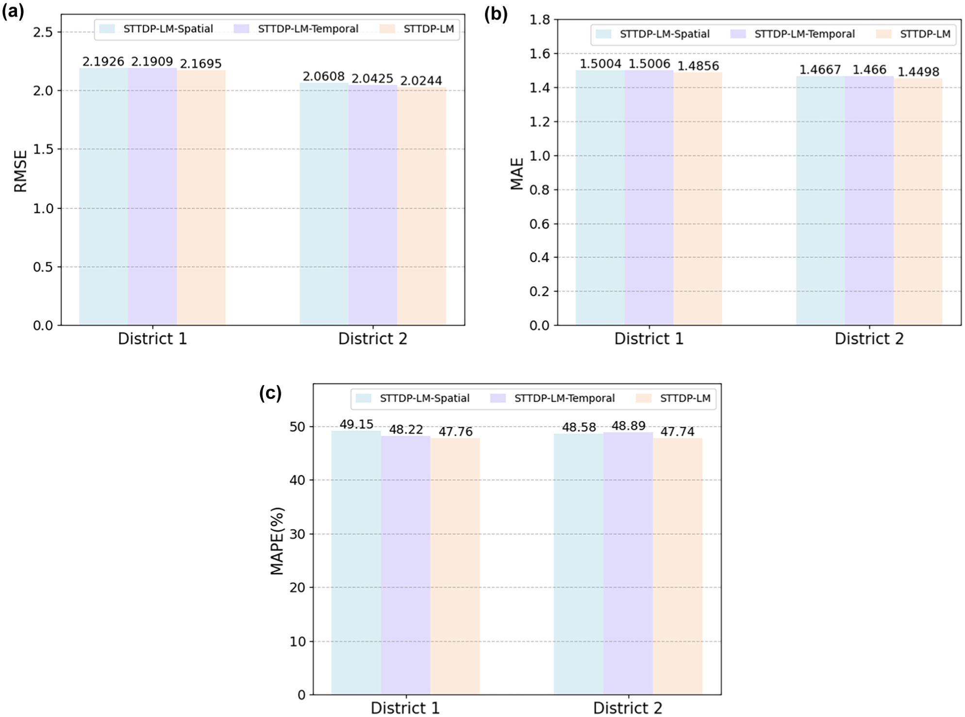
Comparison of prediction results for districts 1 and 2 with consideration of spatial and temporal modeling: (a) root mean square error (RMSE); (b) mean absolute error (MAE); (c) mean absolute percentage error (MAPE).
Prediction Performance with Limited Data
To evaluate the prediction performance with limited data of the STTDP-LM, two experiments are designed and conducted. In the first experiment, the STTDP-LM is trained with datasets having different training ratios (1%, 5%, 10%, 15%, 20%, 25%, 30%); the results are presented in Figure 7. In the second experiment, all methods are compared using only 1% of the training data; the results are displayed in Figure 8. Limited data refers to the temporal dimension and data volume dimension. With respect to the temporal dimension, the proposed model predicts future demand based on the actual demand values from the past 12 time slices, meaning it only uses data from the past 2 h. With respect to data volume, we fine-tuned the model using 1%, 5%, 10%, and 30% of the training data, respectively.
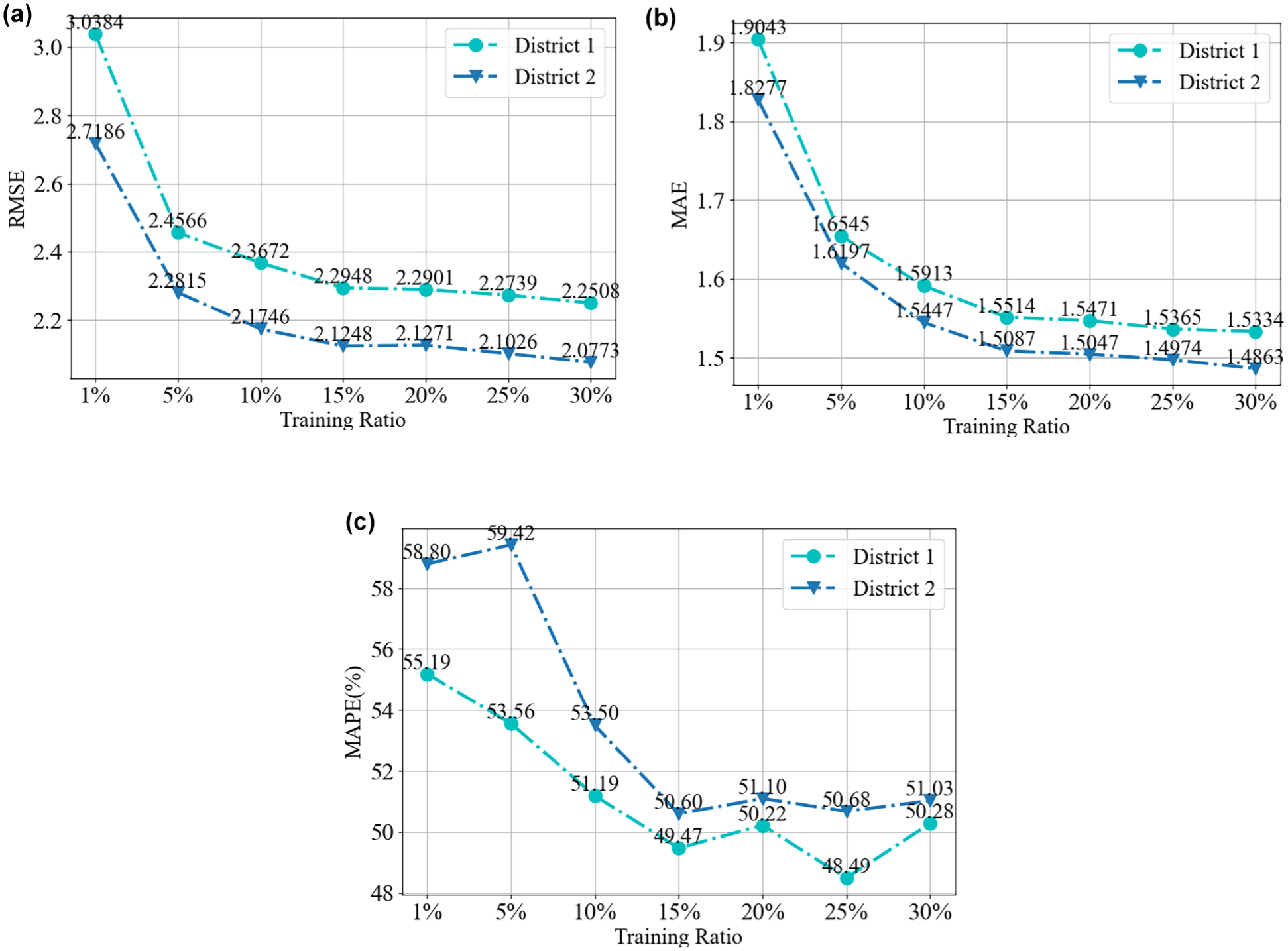
Spatio-temporal taxi demand prediction large model prediction results for districts 1 and 2 with datasets having different training ratios (1%, 5%, 10%, 15%, 20%, 25%, 30%): (a) root mean square error (RMSE); (b) mean absolute error (MAE); (c) mean absolute percentage error (MAPE).
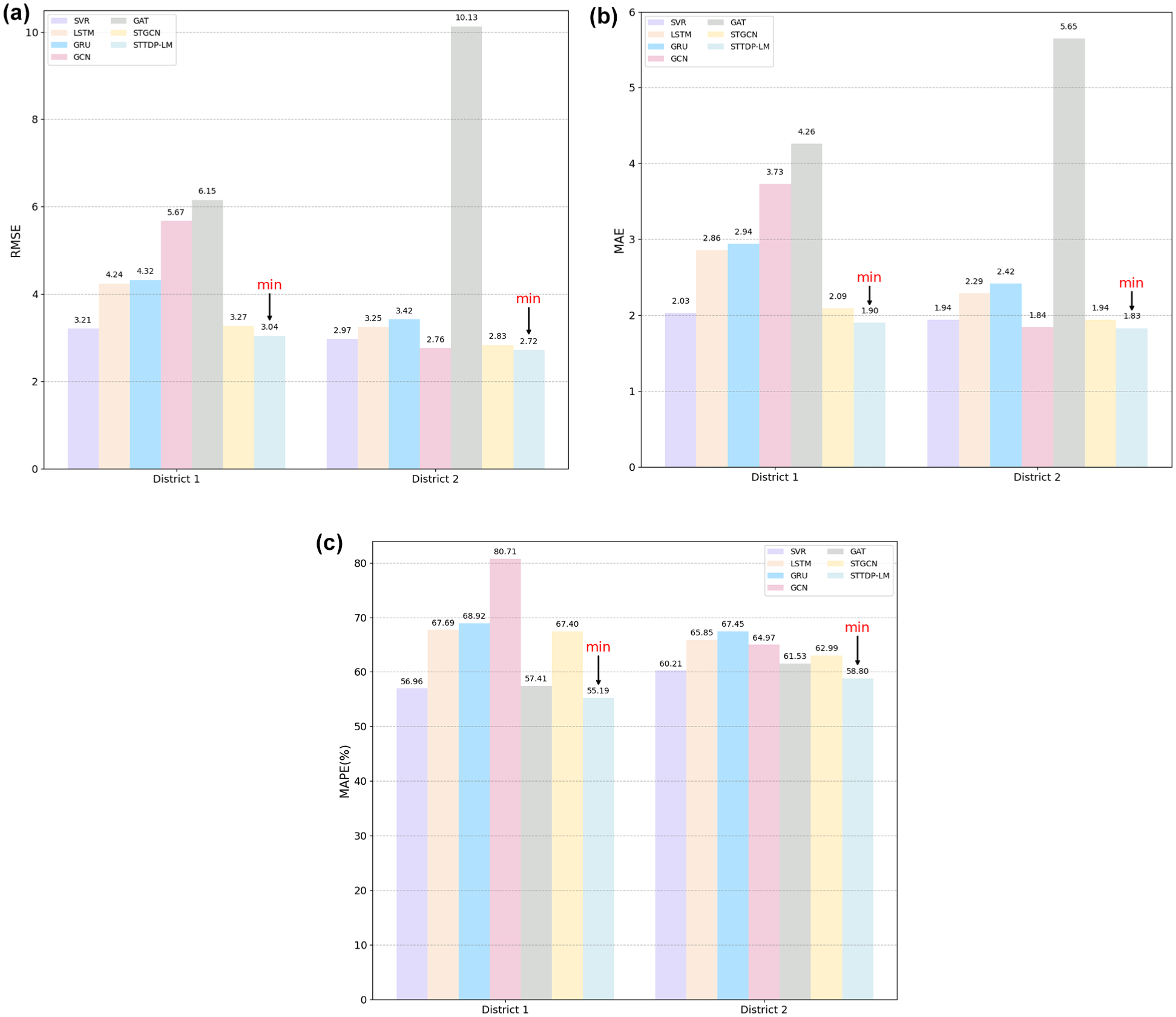
Comparison of prediction results for districts 1 and 2 using different methods with 1% of the training data: (a) root mean square error (RMSE); (b) mean absolute error (MAE); (c) mean absolute percentage error (MAPE).
According to Figure 7, the findings indicate a clear trend: as the proportion of training data increases, the RMSE, MAE, and MAPE values generally decrease, demonstrating improved prediction accuracy. For instance, with 1% of the training data, the RMSE, MAE, and MAPE results in district 1 are 3.0384, 1.9043, and 55.19%, respectively. In district 2, the corresponding values are 2.7186, 1.8277, and 58.80%, respectively. These results outperform the baselines in both districts, as shown in Figure 8. The compared methods are evaluated using training, validation, and testing sets with a 6:2:2 split ratio. When the training data increases to 20%, the prediction results in district 1 improve, with RMSE, MAE, and MAPE values of 2.2901, 1.5471, and 50.22%, respectively. The results surpass the performance of baselines that use all training data, including the ARIMA, LSTM, GRU, GAT, GCN, and STGCN. In district 2, the corresponding results are 2.1271, 1.5047, and 51.10%, outperforming the baseline methods, including the ARIMA, LSTM, GRU, GAT, and GCN.
As shown in Figure 8, the proposed method achieves significantly higher prediction accuracy compared to all baseline methods, even with a very small proportion of training data (1%). When the training samples are significantly reduced, the comparison methods exhibit a much higher increase in RMSE, MAE, and MAPE values compared to the STTDP-LM. Notably, the MAPE value of the ARIMA exceeds 1000, which is an invalid result. Excluding the ARIMA, other comparison methods show increases in the average values of 43.17%, 42.88%, and 21.11%, in district 1, and 47.89%, 41.78%, and 4.98% in district 2. In contrast, the STTDP-LM demonstrates a much smaller increase in the average values of the three indicators, with 28.60%, 21.99%, and 13.46% in district 1, and 25.54%, 20.68%, and 18.81% in district 2.
In summary, the findings highlight the STTDP-LM’s ability to recognize complex patterns from limited data, achieving prediction results comparable to those obtained with sufficient training data. The reason is that traditional and deep learning models rely heavily on the available training data, making them more prone to overfitting when data is sparse. Taxi demand data is often sparse and noisy, especially in certain regions or times. The STTDP-LM uses pre-trained LLMs that have learned broad patterns from large datasets. This allows it to generalize effectively, even with limited taxi demand data. In early deployment scenarios of newly developed areas, where only minimal historical data is available, supervised learning methods often struggle to build effective predictors. In contrast, the STTDP-LM can deliver relatively stable prediction results even under limited data conditions. This makes it particularly valuable for supporting intelligent transportation planning and vehicle dispatch during the early operational stages of urban expansion or redevelopment.
Multi-Step Prediction Performance
Because of the increased complexity of long-term temporal dynamics and the challenges associated with extrapolating historical patterns, multi-step prediction is inherently more uncertain and difficult than short-term prediction. To evaluate the performance of long-term predictions, this study compares the prediction results of the STTDP-LM with several comparable models over the next six time steps. Specifically, the SVR and STGCN are selected as representative models for traditional methods and graph neural networks, respectively. The LSTM and GRU are chosen as representative RNN methods for multi-step prediction. The comparison results for multi-step prediction are presented in Tables 2 and 3.
Multi-Step Prediction Results of District 1
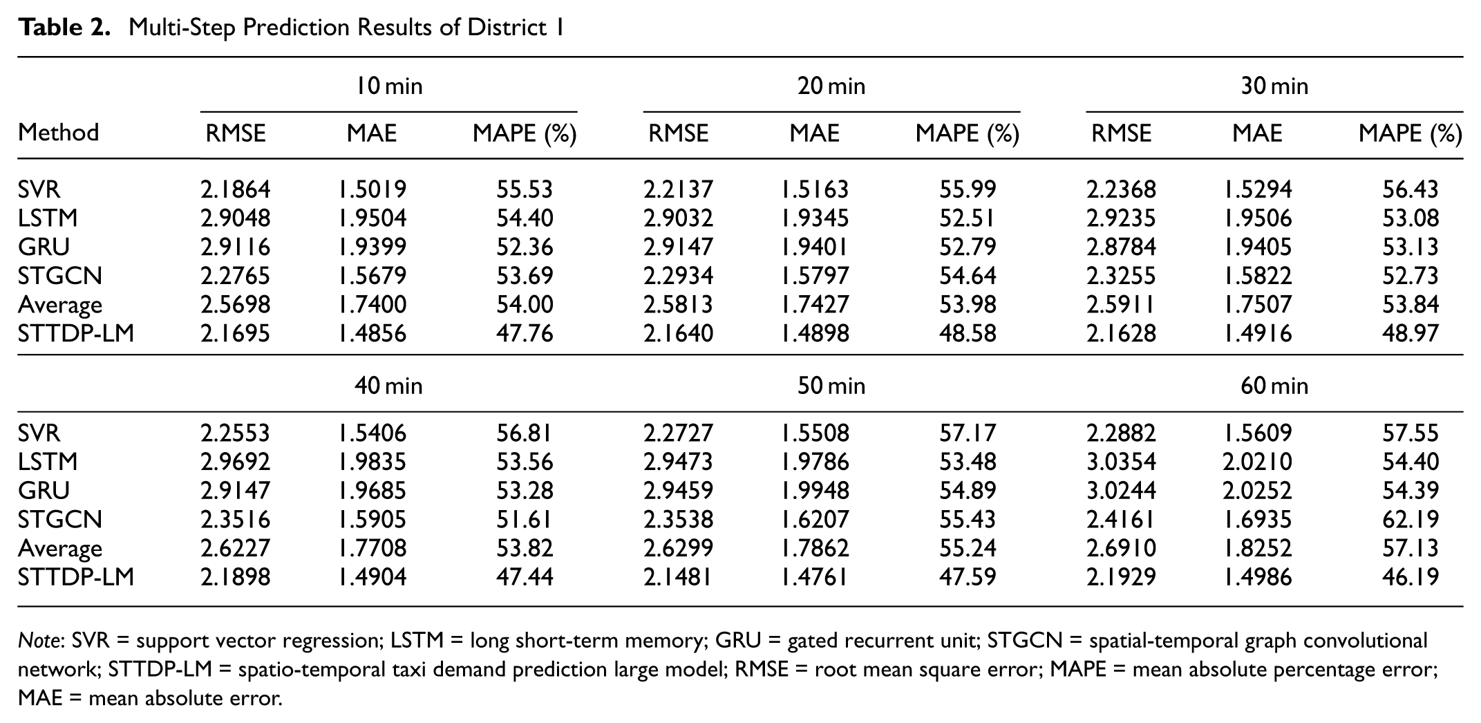
Note: SVR = support vector regression; LSTM = long short-term memory; GRU = gated recurrent unit; STGCN = spatial-temporal graph convolutional network; STTDP-LM = spatio-temporal taxi demand prediction large model; RMSE = root mean square error; MAPE = mean absolute percentage error; MAE = mean absolute error.
Multi-Step Prediction Results of District 2
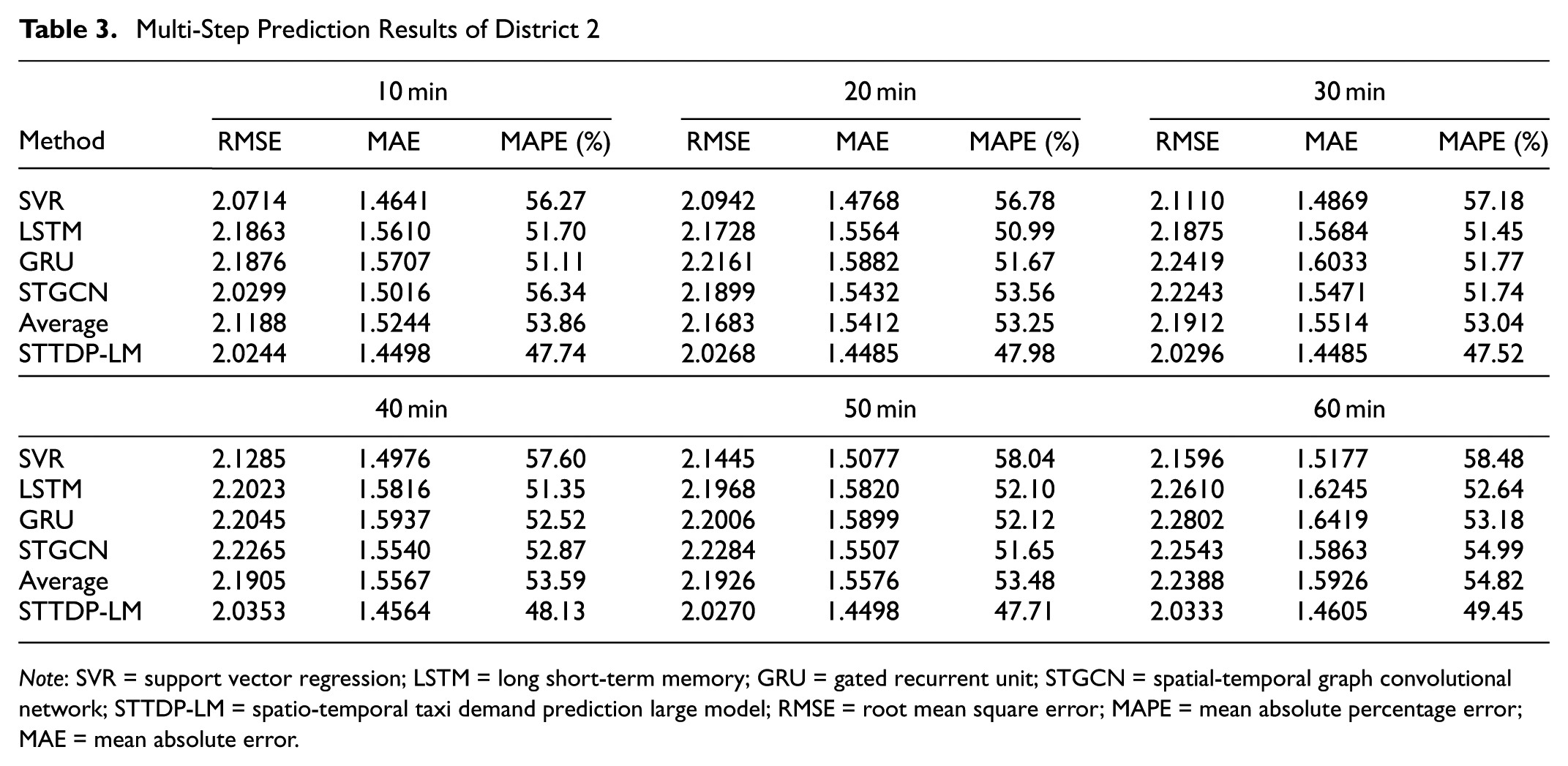
Note: SVR = support vector regression; LSTM = long short-term memory; GRU = gated recurrent unit; STGCN = spatial-temporal graph convolutional network; STTDP-LM = spatio-temporal taxi demand prediction large model; RMSE = root mean square error; MAPE = mean absolute percentage error; MAE = mean absolute error.
The results show that the STTDP-LM outperforms other methods in long-term prediction. In district 1, for a two-step prediction (20 min), the STTDP-LM achieves average reductions of 16.17%, 14.51%, and 10.00% in the RMSE, MAE, and MAPE, respectively. For a six-step prediction (60 min), it achieves reductions of 18.51%, 17.89%, and 19.15%. Similarly, in district 2, for a two-step prediction, the STTDP-LM shows average reductions of 6.53%, 6.02%, and 9.90% in the RMSE, MAE, and MAPE, respectively. For a six-step prediction, it achieves reductions of 9.18%, 8.29%, and 9.80%, respectively.
As the prediction time increases, prediction errors generally grow. With each prediction step, the accumulated error increases. In addition, the nonlinearity and fluctuations in the demand data become more complex. As shown in the graph, the STTDP-LM’s error grows more slowly than the comparison methods as the prediction step increases. The difference becomes especially noticeable after the fifth step. This improved performance is because of the prior knowledge learned from extensive LLM training. Furthermore, the STTDP-LM enhances the model’s ability to capture long-term dependencies in taxi demand data.
Model Parameter Analysis
For the proposed model, the parameter
Prediction Results with Varying Values of Unfrozen Layers U
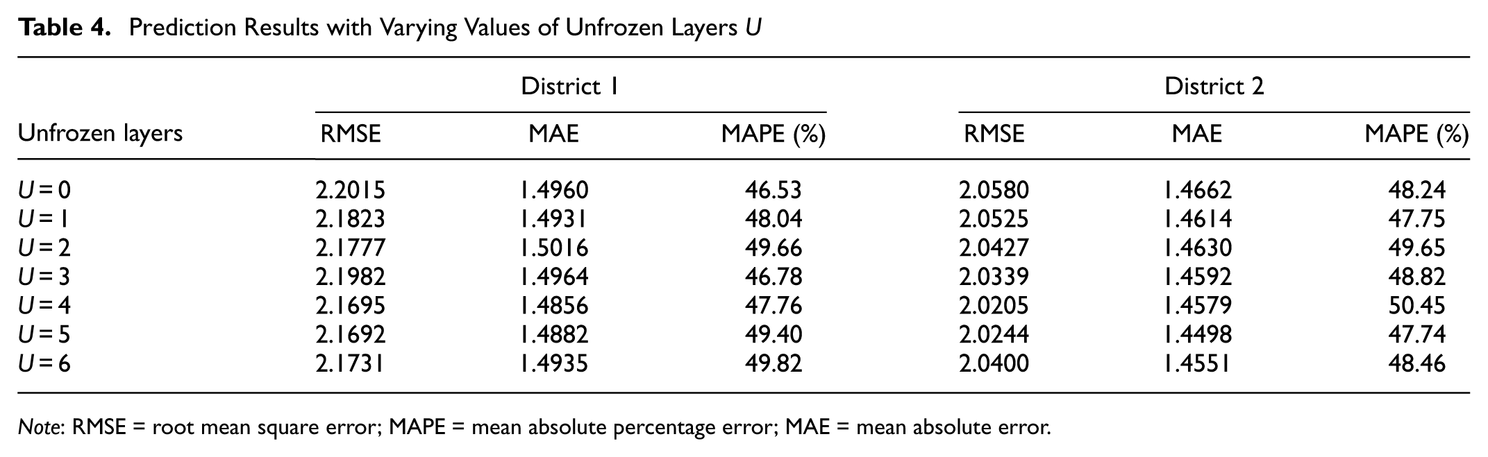
Note: RMSE = root mean square error; MAPE = mean absolute percentage error; MAE = mean absolute error.
The reason for this is that the pre-trained weights of the model are typically trained on large amounts of data. Generally, freezing the lower layers of the model (such as the first few layers of a transformer) is preferred, as these layers tend to learn more general features. The unfrozen layers, on the other hand, update their parameters during fine-tuning, allowing the model to learn features that are more specific to the task of demand prediction. The frozen layers remain unchanged to preserve the pre-trained knowledge and avoid its loss during fine-tuning, while also reducing computational overhead and training time. In this experiment, the STTDP-LM has six layers in total. The number of unfrozen layers is set to 4 for district 1 and 5 for district 2 to adjust the model’s parameters and improve its adaptation to the demand prediction task.
Conclusions
This study presents a novel taxi demand prediction approach using GPT-2 to capture complex spatio-temporal dependencies, even with limited historical data. The model integrates road network topology and employs fine-tuning techniques to improve prediction accuracy. Experimental results show that the STTDP-LM outperforms traditional and deep learning models, achieving significant reductions in key metrics. The importance of both spatial and temporal modeling is also verified. The STTDP-LM performs well even with very limited training data (1%). It also shows strong capabilities in multi-step prediction. This makes it especially useful in real-world applications where data is scarce. In conclusion, the STTDP-LM provides an effective and robust solution for taxi demand prediction, particularly in areas with limited historical data.
Spatial and temporal dependencies are effectively captured using GATs and multi-scale modeling. However, adding factors such as weather, holidays, and other contextual influences could improve the model further. Future work will focus on integrating these contextual features into a spatio-temporal large model, particularly for non-typical demand patterns and more dynamic environments. In addition, we also plan to explore and compare the performance impacts of integrating other large models into our framework.
Footnotes
Author Contributions
The authors confirm contribution to the paper as follows: study conception and design: J. Chen, C. Yuan; data collection: Y. Wang, R. Li, C. Zong; analysis, and interpretation of results: M. Zhang, Z Chen; draft manuscript preparation: J. Chen, Y. Wang. All authors reviewed the results and approved the final version of the manuscript.
Declaration of Conflicting Interests
The authors declared no potential conflicts of interest with respect to the research, authorship, and/or publication of this article.
Funding
The authors disclosed receipt of the following financial support for the research, authorship, and/or publication of this article: The research was supported by the Scientific Innovation Practice Project of Postgraduates of Chang’an University (Grant No. 300103725056) and the Natural Science Basic Research Plan in Shaanxi Province of China (Grant No. 2021JC-27).