
Abstract
Road networks are often subjected to disruptions caused by demand and capacity uncertainties, leading to excessive delays. A resilient transport system could absorb and recover quickly from such events. However, resiliency varies across different links, which may be because of zonal characteristics, network structure, or other factors. This study develops a methodology to quantify road network resilience at the zonal level and identify factors affecting it. Crowdsourced traffic speed data from approximately 33,000 locations was used to calculate resilience metrics, including the zonal resilience index, zonal vulnerability index, and zonal recoverability index. These metrics were modeled using geographically weighted regression to explore their relationship with independent variables. The results revealed that zonal trip heterogeneity, land use heterogeneity, and road category heterogeneity within a zone significantly reduce resilience.
In contrast, connectivity measures, such as the clustering and degree assortativity coefficients, improve the recoverability of the zone. The increase in households owning more than two motorized vehicles in a zone reduces zonal resilience. The models were validated using subsets of the data, splitting weekdays from June 1–15 and June 16–30 and testing the model under different zone sizes. Results showed consistent variable effects across subsets and configurations, with slight variations in the significance of certain factors. Policymakers can utilize these insights to create land use or congestion pricing policies for individual zones to curb congestion. In addition, the network topology results can help plan a resilient road network for developing cities.
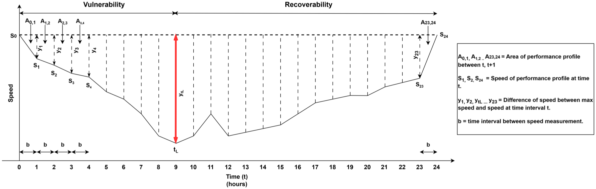
Road networks are often subjected to disruptions caused by demand and capacity uncertainties, traffic incidents, and road maintenance work. These events lead to excessive delays ( 1 – 3 ), travel time unreliability ( 4 , 5 ), increased emergency vehicle response times ( 6 , 7 ), and increased emission and fuel consumption ( 8 ). One approach for evaluating road network performance under such routine day-to-day disruptions is based on the concept of resilience, which is the ability of the system to absorb the impact of disruptions and return to a pre-event state or a newer equilibrium state. Resilience is represented using an apex downward triangle, where the area of the triangle indicates the loss of performance over time during the disruption ( 9 ). The downward-sloping part of the curve shows degradation in performance, known as vulnerability, and the upward sloping indicates recoverability (Figure 1).
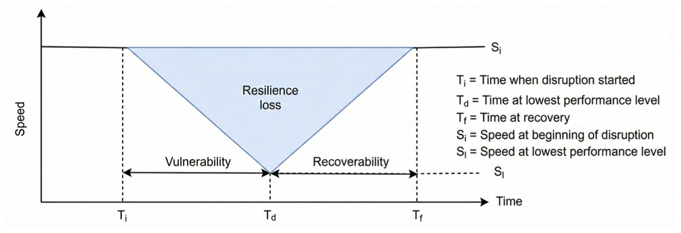
Typical resilience triangle and its components.
A resilient transport system could absorb and recover quickly from day-to-day disruptions. However, a transport network cannot be completely resilient; certain road links recover quickly, and others take longer. This difference in recovery can be because of zonal or macro level characteristics, such as land use distribution, intersection density, and street layout, which influence traffic composition and flow variation. In addition, resilience can be affected by link or micro level characteristics, such as on-street parking, bus stops, pedestrian crossings, and traffic signals.
Road network resilience in the existing literature has been quantified using topological, attribute, and performance-based measures ( 10 ). For methods, resilience has been quantified using topology, simulation, and data-driven methods ( 11 ). This study quantifies resilience using a data-driven method and performance-based measures. The topological approach considers network topology and graph-based metrics, such as centrality ( 12 ), the giant component ( 13 ), average node degree ( 14 ), and others, to quantify network connectivity and identify important nodes and edges. Attribute-based metrics, such as the travel time index ( 15 ), mobility ( 16 ), and recovery rate ( 17 ) have been used to measure resilience from the perspective of robustness, redundancy, resourcefulness, and rapidity (the 4Rs). Finally, performance-based metrics, such as satisfied travel demand and the time-dependent ratio of the recovery loss ( 18 ), have been used to measure resilience for the period affected by the disruption.
Many studies have explored road network resilience; they typically focus on natural disasters or rely on hypothetical simulations ( 19 – 22 ). In contrast, performance loss because of recurring daily traffic variations remains underexplored in the resilience context. In addition, link-level approaches dominate the literature, and a zonal perspective may provide a more actionable understanding of resilience patterns influenced by macro level urban characteristics.
In this study, vulnerability is defined as the extent of performance loss experienced during the degradation phase of a disturbance, measured by the area under the performance drop curve from the onset to the lowest point. Recoverability is the system’s ability to regain performance after disruption, measured by the area under the curve during recovery. Resilience, is the system’s ability to minimize total performance loss across the degradation and recovery phases. These definitions are consistent with performance-based frameworks adopted in some studies ( 9 , 19 ).
The objective of this study is to develop a zonal-level methodology to quantify road network resilience under routine day-to-day disruptions and identify the key factors influencing vulnerability, recoverability, and resilience across zones. The insights from this study aim to guide targeted policy interventions, such as congestion pricing, land use planning, and evacuation strategies.
Unlike previous studies that often analyze resilience in large-scale disasters or hypothetical scenarios, this study evaluates performance loss because of routine, day-to-day disruptions using real-world, crowdsourced traffic data. The resilience metrics vulnerability index (VI), recoverability index (ReI), and resilience index (RI) are adapted from previous studies; their application at the zonal level using average weekday speed profiles for over 32,000 points across Sydney, Australia, is novel. Furthermore, the spatial heterogeneity in resilience is modeled using geographically weighted regression (GWR), which captures the influence of zonal characteristics (e.g., land use entropy [LCE], trip heterogeneity, and network structure), a dimension underexplored in previous work.
Literature Review
Numerous approaches have been employed in the literature to assess road network vulnerability and resilience. These approaches can broadly be categorized into topological, attribute-based, and performance-based frameworks. In addition, recent work has focused on resilience during large-scale disruptions, and relatively few studies have examined resilience under recurring daily congestion patterns. The following paragraphs in this section will provide an overview of the relevant studies, highlight gaps in the existing literature, and identify how this study addresses them.
Most studies on the resilience approach have focused on assessing the road network performance under natural disasters. For instance, Calvert and Snelder ( 20 ) used the loop detector volume data to analyze the resilience of two corridors during heavy rain in Rotterdam, the Netherlands. They developed a new resilience metric, the link performance index for resilience (LPIR), which is a function of volume, the duration of the disruption, and the speed change. They compared the results of the LPIR with two common performance measures (i.e., delay time and recovery time). The results showed that many areas identified as underperforming in the LPIR were flagged as normal by other metrics. Niu et al. ( 19 ) used crowdsourced data from three hurricanes, one dam spill, and a carnival to evaluate link resilience using performance-based metrics. They assessed the effect of network structure and link attributes. They found that link characteristics, such as the number of lanes, betweenness and degree centrality (DC), significantly affected the resilience. Wang et al. ( 21 ) evaluated the resilience of public transport systems during COVID-19, and measured resilience by considering ridership as a resilience measure. The results showed that the resilience of the transit system was significantly affected by the user’s age and whether the user is a commuter. Yichi et al. ( 22 ) analyzed the spatial variation in road network vulnerability and found that although spatial autocorrelation existed, it was there for contiguous links. In addition, they developed a probit model by dividing the vulnerability measure into different categories and found that micro level network metrics affected the vulnerability. A few studies ( 23 , 24 ) have utilized a zonal approach to assess the vulnerability of road networks against disruptions on the Swedish road network. The authors divided the study area into multiple grids to analyze the impact of disconnecting the road network within each grid from the rest of the network. In addition, they compared the effects of area-wide disruptions with those of individual link failures. The findings showed that area-wide disruptions are primarily driven by the level of internal, outbound, and inbound travel demand within the affected area. In contrast, individual link failures are more significantly influenced by the flow on that specific link and the redundancy of the surrounding network.
Despite the potential benefits of a resilience-based approach, its use in quantifying the effect of frequent, day-to-day disruptions has been limited. Sullivan et al. ( 25 ) evaluated the robustness of the network using a capacity reduction approach by removing links from a hypothetical network and measuring the impact on total network travel time. Gauthier et al. ( 12 ) developed a methodology for identifying the critical links subjected to day-to-day disruptions using unweighted and travel time-weighted betweenness centrality and found that the links with higher centrality values are more critical for the network. Akbarzadeh et al. ( 26 ) quantified the resilience of the urban road network of a city in Iran by comparing the relation between traffic flow and centralities. They found that network structure strongly relates to traffic flow, and resilience depended more on link capacities than on betweenness, flow, or congestion level. Another study that assessed the performance loss, propagation, and dissipation of congestion was conducted by Nair et al. ( 27 ) for 40 cities worldwide. They evaluated the performance loss using the congestion index, and its propagation and dissipation were calculated as the change in congestion index in an hour. They found that the performance loss was significantly related to the cities’ gross domestic product per capita and population density. In addition, the congestion propagation and dissipation analysis were limited to clustering cities based on these parameters.
The literature review shows that the resilience-based approach has been primarily used in research on natural disasters. These studies have improved our understanding of the resilience of road networks to disasters. However, the effect of travel demand fluctuation on the performance loss of road networks has not been explored through the lens of resilience. Although the travel demand fluctuations are expected and natural in a road network and not as severe as natural disasters, they are recurring and can congest the road network, leading to significant performance loss. These conditions are not disruptive in the conventional sense (e.g., accidents or extreme events); they are treated as routine performance stressors that impair system efficiency and require recovery. Therefore, it justifies a resilience-based framework. Under day-to-day conditions, the free flow state represents the “predisruption” baseline. The period from the initial drop in speed to the lowest point is defined as the vulnerability phase. In contrast, the subsequent return from the lowest speed toward free flow conditions defines the recoverability phase. Therefore, this study will focus on quantifying the resilience of a road network at a zonal level under day-to-day traffic using crowdsourced traffic data and model the impact of different zonal characteristics. Although some studies utilize crowdsource data for congestion, they are limited and have used conventional measures to assess the congestion and not a resilience-based approach.
The other research gap observed is that most studies have focused on link-level resilience, and the independent variables considered are link characteristics. In addition, the existing studies that have employed zone-based vulnerability have focused on hypothetical disruptions and not real-world traffic data. Furthermore, the disruptions represented the closure of a zone by disconnecting it from the rest of the zones and analyzing its impact on zone-to-zone travel times. However, the effect of zonal characteristics, such as land use, demographics, socioeconomic factors, overall street layout, and public transport facilities, has not been considered, and these factors may play a crucial role in shaping traffic patterns and, therefore, the resilience of the road network. For instance, areas with mixed land use may experience varying levels of congestion throughout the day, affecting their ability to recover from disruptions compared with more homogenous zones.
In contrast to previous studies, the methodology in this study is designed to assess the resilience of the road network using link-level speed data, which is then aggregated to the zonal level. This approach does not account for the disconnection of a zone or analyze changes in zone-to-zone travel times because of zone closures. Instead, it evaluates the zone’s resilience, independent of these disruptions. In addition, this study quantifies the vulnerability and recoverability of the road network; however, the area-covering vulnerability can only measure the vulnerability.
The zonal-level analysis enables researchers to assess road network resilience at a finer spatial resolution than traditional network-level assessments. By leveraging these insights, policymakers can develop targeted zone-specific policies, including land use planning, congestion pricing strategies, evacuation procedures, and traffic management solutions. The data reflects routine conditions, identifying zones with lower resilience may also offer valid inputs for preparedness planning under high-demand scenarios, such as evacuations.
This study assesses the zonal resilience of the predefined administrative zones of Sydney, Australia, using speed profiles obtained at different locations on the road network. Data and Methodology section discusses the data set, the methodology for calculating the resilience indices and different zonal factors respectively. Descriptive statistics and spatial autocorrelation section discusses the descriptive statistics of various variables, their correlation, and the spatial autocorrelation. GWR model section discusses the details of the geographically weighted regression model and its results. Model calidation section details the validation methodologies and GWR model results validation. Conclusion section provides the study’s conclusion and how the results can be helpful to policymakers.
Data
The study area in this study encompasses the Central Business District (CBD) of Sydney, Australia, with an area of 344.25 km2. It is composed of 82 Statistical Area Level 2 (SA2) zones, which generally have an average population of 10,000 ( 28 ). The extent of the study area can be seen in Figure 2. In addition, a histogram depicting the count of observations at specific latitude–longitude coordinates is shown, offering insights into the spatial density of the data points. The details of the different data sets used in this study are discussed in the following subsections.
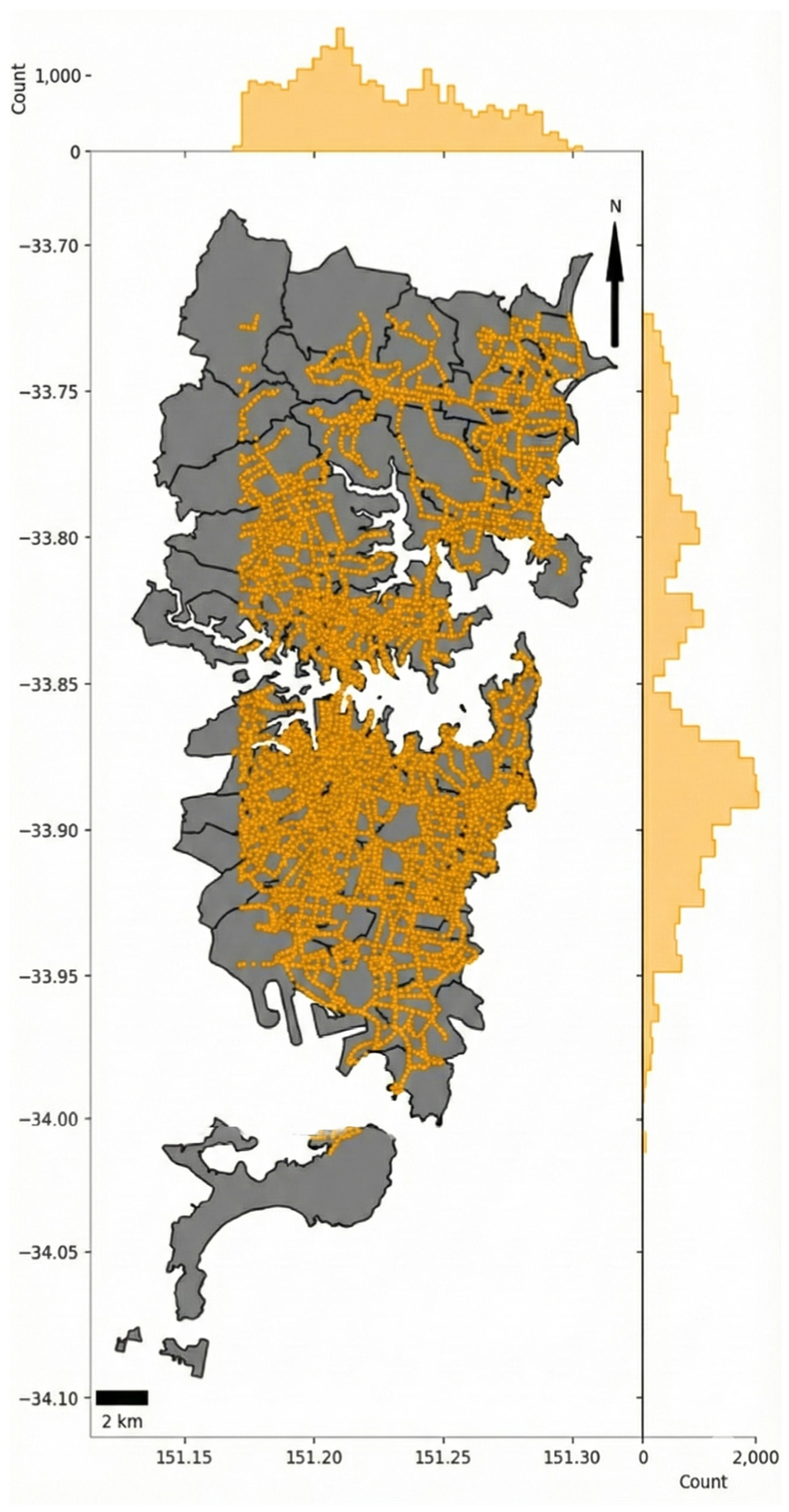
Sydney area and geometric change points.
Speed Data
The speed data for the study area was obtained using the Google Maps Speed Application Programming Interface (API) (now deprecated) at geometric change points (GCP) along the road links, such as merging, diverging, or intersections ( 29 ). The speed data was collected at 32,537 GCPs for 30 days, from June 1, 2018, to June 30, 2018, at 10-min intervals. More details of the data collection procedure can be found in the literature ( 27 ). Although the API used is no longer available, similar data can now be sourced from platforms such as TomTom Traffic Stats ( 30 ), HERE Technologies ( 31 ), or INRIX ( 32 ), as well as from fleet-based GPS aggregators.
Road Network
The road network data for the study area was obtained from OpenStreetMap using the OSMnx Python module ( 33 ) and the Rapidex tool ( 34 , 35 ). The length of the road network considered was 3046 km, with six road categories, the names and percentage share of which are: motorway (5.54%), trunk (4.32%), primary (9.06%), secondary (6.58%), tertiary (12.02%), and residential (62.22%).
Land Use, Demographic, Socioeconomic, and Transportation Data
Data on land use, demographic, socioeconomic, and work-trip characteristics were obtained from the Australian Bureau of Statistics ( 36 ), and data on public transportation were obtained from the open-source General Transit Feed Specification database ( 37 ).
Methodology
The methodological framework adopted in this study had three components. First, average weekday speed profiles at GCPs were used to compute three resilience metrics: (1) VI; (2) ReI; and (3) RI, based on the performance triangle approach. These point-level metrics are aggregated to 82 administrative zones to derive zonal-level resilience indicators (zonal resilience index [ZRI], zonal vulnerability index [ZVI], and zonal recoverability index [ZReI]). Second, a comprehensive set of zonal variables was compiled reflecting road network structure, LCE, population density, transit accessibility, and motorization levels. Finally, a GWR was applied to model the spatially varying relationships between zonal attributes and resilience indicators, accounting for spatial autocorrelation. This integrated zonal approach facilitates spatially targeted resilience planning and extends the application of performance-based resilience metrics to a finer resolution than previous studies. Figure 3 shows the methodological flow in pictorial format.
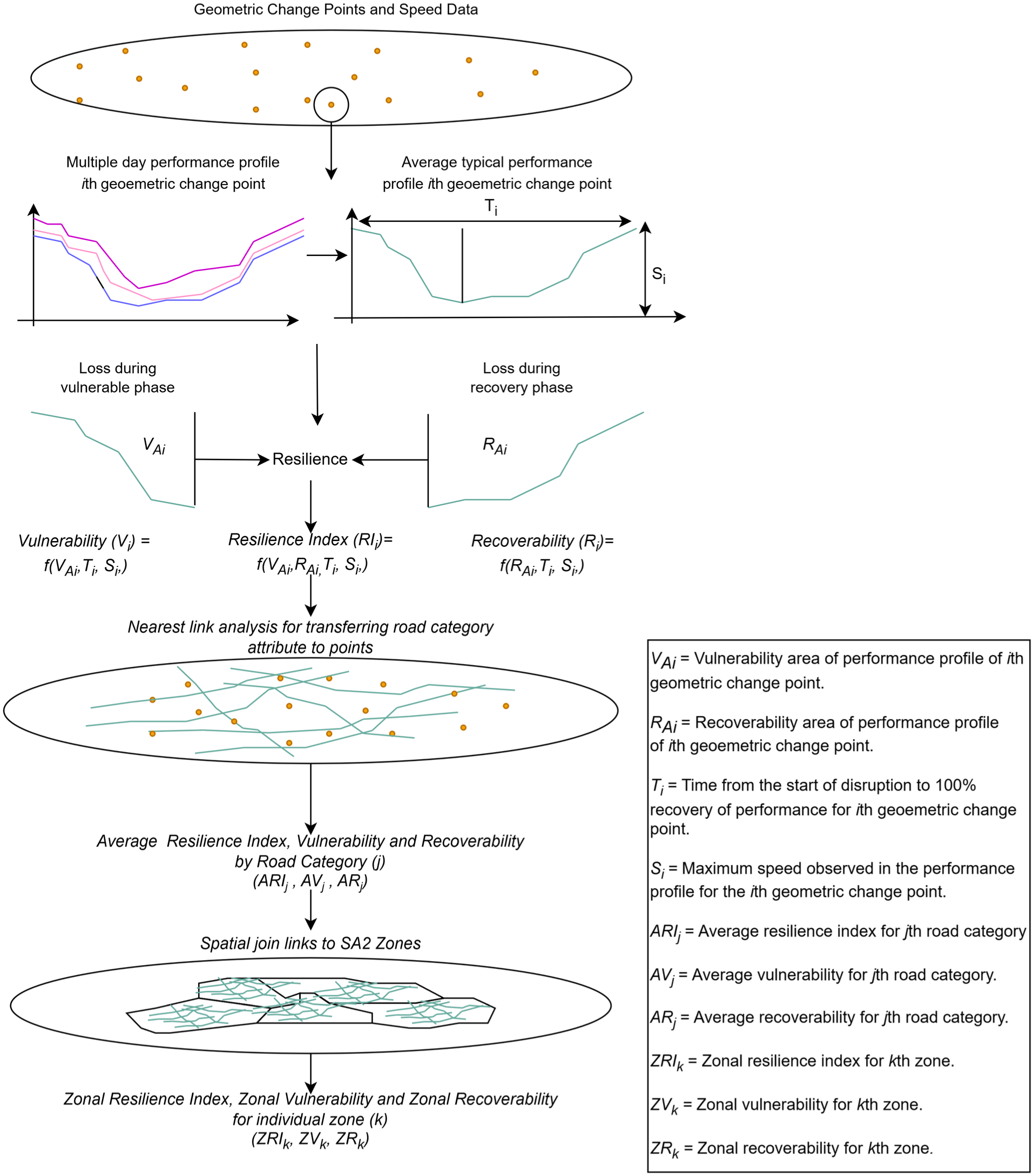
Methodology for zonal-level resilience metrics.
To ensure the robustness of the findings, the model results are validated using two approaches: (1) temporal subsets of data from different parts of the month; and (2) alternative zone configurations created by merging neighboring zones. These checks help confirm the consistency of variable effects across time and spatial scales.
The selected metrics, VI, ReI, and RI, were chosen for their interpretability and effectiveness in quantifying performance degradation and recovery phases. These metrics have been previously validated in disaster resilience studies ( 9 , 19 ). However, this study advances their application by computing them at high spatial granularity (GCP-level) and aggregating them to analyze zonal-level performance, enabling integration with planning and policy tools such as congestion pricing.
Speed Data
The speed data served as the basis for quantifying performance loss. This data was available at the point level and was further processed to compute resilience, vulnerability, and recoverability metrics at the zonal level, as discussed in the following subsection. The methodology consisted of collecting speed data across the Sydney Road network. The speed data were collected at geometric change points over 30 days in June 2018. A total of 21 weekdays were observed out of 30 days in June 2018. These weekday speed profiles were averaged for each GCP to create 32,537 typical weekday speed profiles. Figure 4a shows the 10-min speed profile for different dates for a GCP, and Figure 4b shows the average 10-min weekday speed profile for the same GCP. The average 10-min weekday speed profile is used to calculate the average weekday hourly profile shown in Figure 4c.
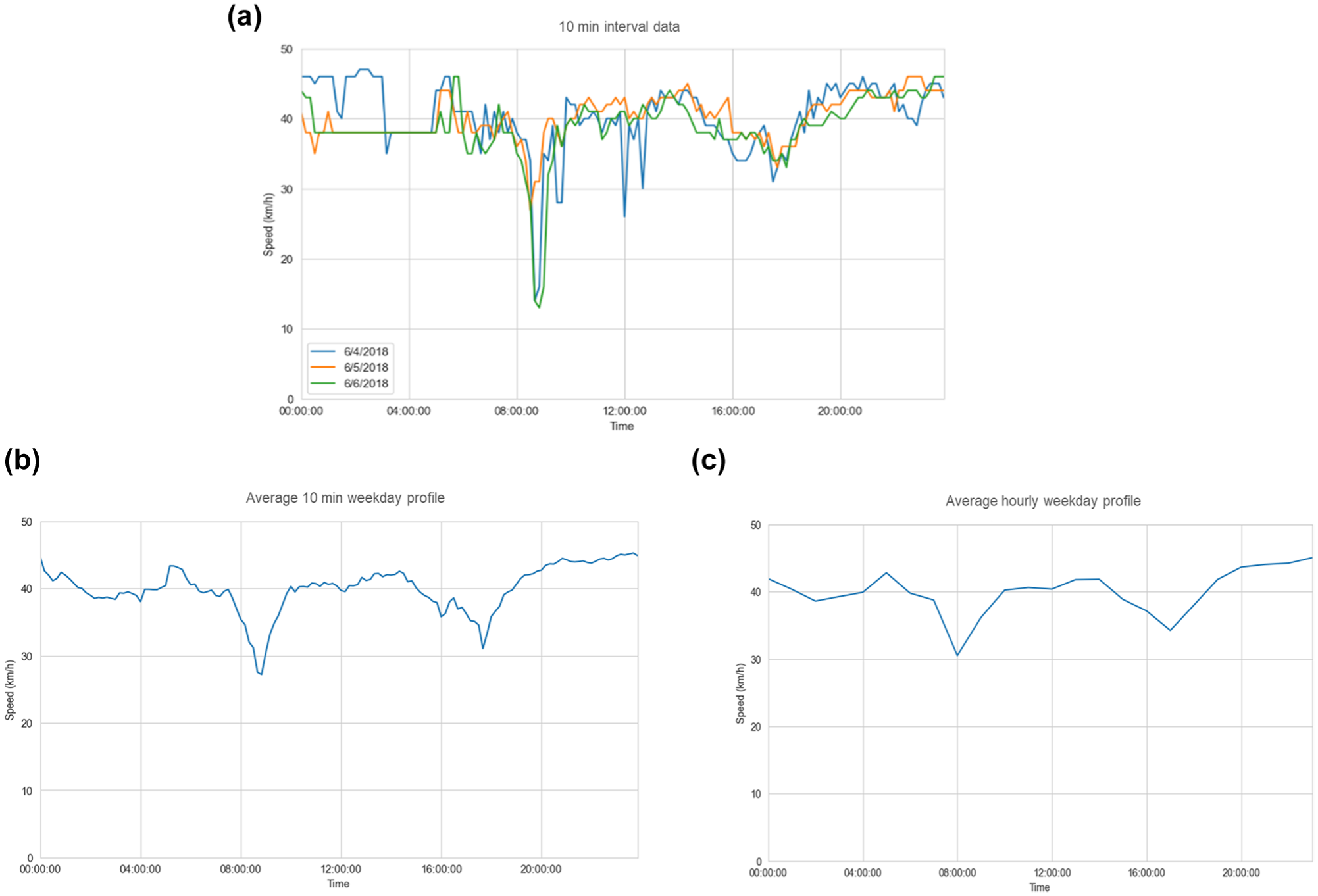
Speed profiles: (a) 10 min interval data speed profile; (b) average 10 min weekday profile; (c) average hourly weekday profile.
The average weekday profiles were used to compute the vulnerability, recoverability, and resilience indices at the point level. Using QGIS, these GCPs were associated with the nearest road links to transfer relevant link attributes, such as road category characteristics, to each point. Then, the GCPs were spatially joined to their corresponding zones, enabling the calculation of zonal-level vulnerability, recoverability, and resilience indices.
Calculating Point Level Vulnerability, Recoverability, and Resilience
In the first step of the resilience analysis, the average weekday speed profiles at each GCP were used to calculate performance loss during the disruption and recovery phases. These profiles were used to derive point-level values of vulnerability, recoverability, and overall resilience using the concept of a resilience triangle. A hypothetical performance profile is shown in Figure 5 to help us understand the calculation of resilience and its components.
Hypothetical performance profile.
The resilience triangle can be divided into multiple trapezoids to simplify calculating the VI, ReI, and RI. To calculate these indices, first, the area of the curve for different phases needs to be calculated, for which the area of individual trapezoids must be calculated. The area of a single trapezoid between time t and t + 1 can be calculated using Equation 1.

where

where
The VI is calculated as the ratio of performance loss during the degradation/vulnerable phase to the theoretical possible loss in 24 h, and the performance loss is measured from
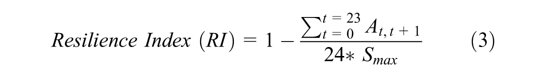
The RI is the ratio of actual and theoretical total performance loss. Based on the previous explanations, the actual total performance loss is calculated as the sum of loss during the vulnerability and recoverability phases ( 19 , 38 ). The RI is calculated using Equation 3. The value of RI varies ranges from zero to one, with a value closer to zero indicating low resilience and high overall performance loss and a value close to one indicating high resilience and low-performance loss.
To further understand the previous indices for the VI, ReI, and RI, three hypothetical speed profiles are shown in Figure 6. Figure 6a shows a profile where the speed drops from 50 km/h to 30 km/h (the lowest speed) over 4 h, and this portion represents the vulnerability. The vulnerability loss was calculated as the area of the vulnerability triangle, for instance, 20 units ((50 – 30)×4×0.5), and the total possible loss was calculated as 1,200 units (50*24). Using Equation 2, the VI was 0.03 (40/1,200). Similarly, it takes 20 h to recover, representing a loss during recovery. Using Equation 2, the ReI was 0.17; Equation 4 calculated the RI as 0.8. The VI and ReI indicate low-performance loss at 3% and 17% of the theoretical possible loss, respectively, and therefore a high resilience. However, looking at the loss dynamics, the maximum loss occurs during the recoverability phase, indicating a slower recovery. Similarly, for Figure 6b, the VI, ReI, and RI were 0.25, 0.05, and 0.7, respectively, indicating that Figure 6b is less resilient than Figure 6a because of a lower RI value as well as higher VI and ReI. However, the dynamics of performance loss are different in Figure 6b, where the recoverability loss is lower than the loss during vulnerability. This indicates a quicker recovery. Figure 6c shows a balanced profile with equal loss during the vulnerability and recoverability phase. The VI, ReI, and RI for Figure 6c were 0.2, 0.2, and 0.6, respectively. The indices indicate that Figure 6c has the lowest resilience of the three profiles.
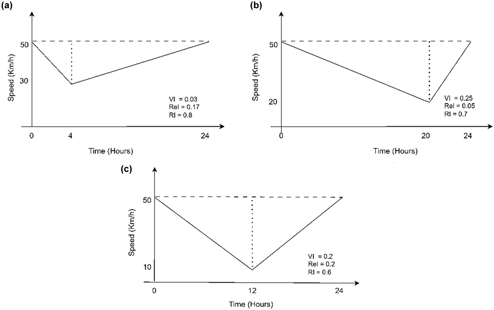
Different hypothetical speed profiles: (a) high vulnerability, (b) high recoverability, and (c) balanced profile.
Calculating VI, ReI, and RI at the Zonal Level
The GCPs were spatially joined with the nearest link and SA2 zones to calculate the zonal metrics. Because the GCPs are located at different links and have different road categories, each GCP is of varying importance. Therefore, to account for these differences, the ZVI, ZReI, and ZRI were calculated using the weighted average rather than a simple average. The weights considered were the speed limit of the nearest link to the GCP. The equations for calculating the ZVI, ZReI, and ZRI for a zone k are given in Equation 5–7, respectively.

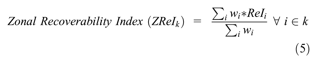
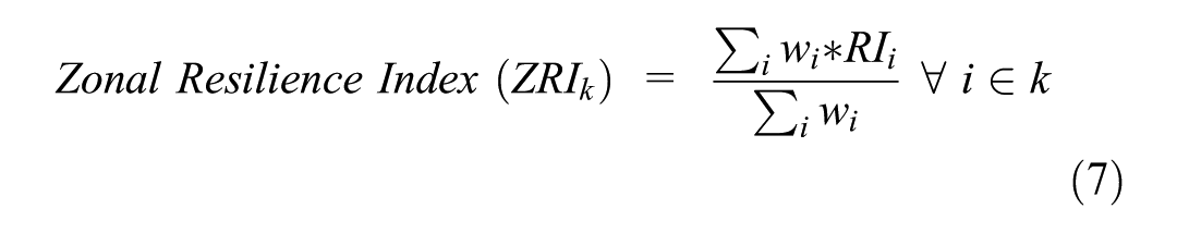
where i represents the ith GCP and
Road Network
The extracted road network was further processed to develop several zonal-level explanatory variables. These include the proportion of road length by category, network density, and graph-based centrality and connectivity measures. These variables help explain how the structure of the road network influences resilience. The details of the derivation and relevance of these variables are described in the following subsections.
Entropy and Density Metrics
A road network consists of multiple road categories, and the traffic performance for roads of different categories is different; therefore, a zone’s resilience may be affected by the type and the heterogeneity of the road categories within it. Therefore, to evaluate the effect of the heterogeneity of road category on resilience, a variable called road category entropy (RCE) was developed ( 1 , 39 ). For calculating the road category heterogeneity, the proportion of six road categories was used in Equation 8.

where
In addition to RCE, the road network has been used to calculate the node density (ND) at the zonal level. The ND at the zonal level is calculated as the ratio of the number of nodes in a zone to the zone area.
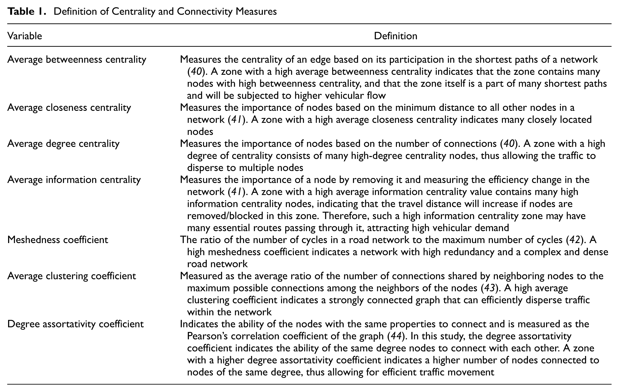
Centrality and Connectivity Measures
As seen in the literature, multiple studies have tried relating the graph theory metrics, such as centrality and connectivity, with resilience at the micro level. However, this study assesses their impacts on zonal resilience. The centrality measures considered include degree, betweenness, closeness, and information, which capture the importance of individual nodes based on position or flow. In addition to centrality, connectivity metrics were included, which reflect how well different network components are structurally connected and how resilient the network is to local or global disruptions.
The meshedness, clustering, and degree assortativity (DA) coefficients are grouped under network connectivity metrics because they describe how well different parts of the network are structurally connected. The meshedness coefficient indicates global redundancy by measuring the proportion of loops in the network. The clustering coefficient (AC) reflects local cohesion by measuring how well a node’s neighbors are interconnected. The DA measures whether nodes tend to connect with other nodes of similar degree, which affects how evenly traffic loads are distributed across the network.
Together, these metrics provide a more complete view of connectivity. All centrality and connectivity measures were first calculated at the node or link level and then at the zone level. The details of these variables are given in Table 1.
Definition of Centrality and Connectivity Measures
Land Use, Demographic, Socioeconomic, and Public Transportation Data
The land use data was used to calculate the land use category entropy by first calculating the proportion of different land uses. The different land uses considered in this study included commercial, educational, hospital, industrial, residential, and transport. Similarly, the proportion of different work trip modes, such as cars, motorbikes, buses and non-motorized modes obtained from the Australian Bureau of Statistics ( 28 ) was used to calculate trip entropy (TE). The other data, such as population and household composition based on vehicle ownership, were used to calculate population density and household proportion with less than or equal to two motorized vehicles (PMV) or household proportion with more than two motorized vehicles (PMV2). The public transport data from general transit feed specification (GTFS) was used to calculate bus stop density (BD) for each zone.
Descriptive Statistics and Spatial Autocorrelation
This section summarizes the resilience metrics at the point and zonal levels and explores their spatial distribution. Descriptive statistics will help understand the overall variation in performance loss across the study area, Pearson correlation helps understand the correlation between variables, and spatial analysis using Moran’s I is used to assess whether resilience patterns exhibit spatial clustering. These steps provide important context before applying the regression models.
Resilience Metrics at Point Level
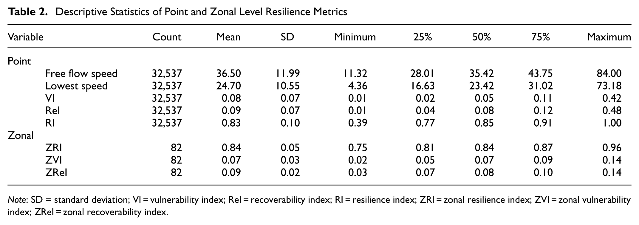
The descriptive statistics of the RI and its components, vulnerability and recoverability, are given in Table 2, along with descriptive statistics of free flow speed, lowest speed, VI, ReI, and RI.
Descriptive Statistics of Point and Zonal Level Resilience Metrics
Note: SD = standard deviation; VI = vulnerability index; ReI = recoverability index; RI = resilience index; ZRI = zonal resilience index; ZVI = zonal vulnerability index; ZReI = zonal recoverability index.
Table 2 shows that the maximum free flow speed observed at the GCPs was 84 km/h, and the minimum free flow speed observed was 11.52 km/h, showing a wide range of variation. For the RI, the average RI is 0.83, indicating the network suffers a loss of 17%, which shows that the overall performance loss is low. In addition, the quantiles indicate that about 25% of the GCPs have a resilience below 0.77. In the VI, the maximum loss attributed to vulnerability was 0.42, and the average loss was 0.08, indicating that out of 100% possible loss, the average loss during vulnerability is 8%. Similarly, the average loss for the ReI is 0.07 (7%). The descriptive statistics show that the average profile is balanced triangular, indicating an equal loss in vulnerability and the recoverability phase. The spatial distribution and histogram for different RI, VI, and ReI ranges are shown in Figure 7. It can help us further understand the location of GCPs with higher loss. The zones central to the map have a very high count of GCPs; it is a CBD area. In addition, the same area contains relatively more GCPs with low RI values, indicating a zone with high-performance loss, which is also visible in the VI (Figure 7b) and ReI (Figure 7c). However, the number of GCPs having an RI (0.39–0.51) is small.
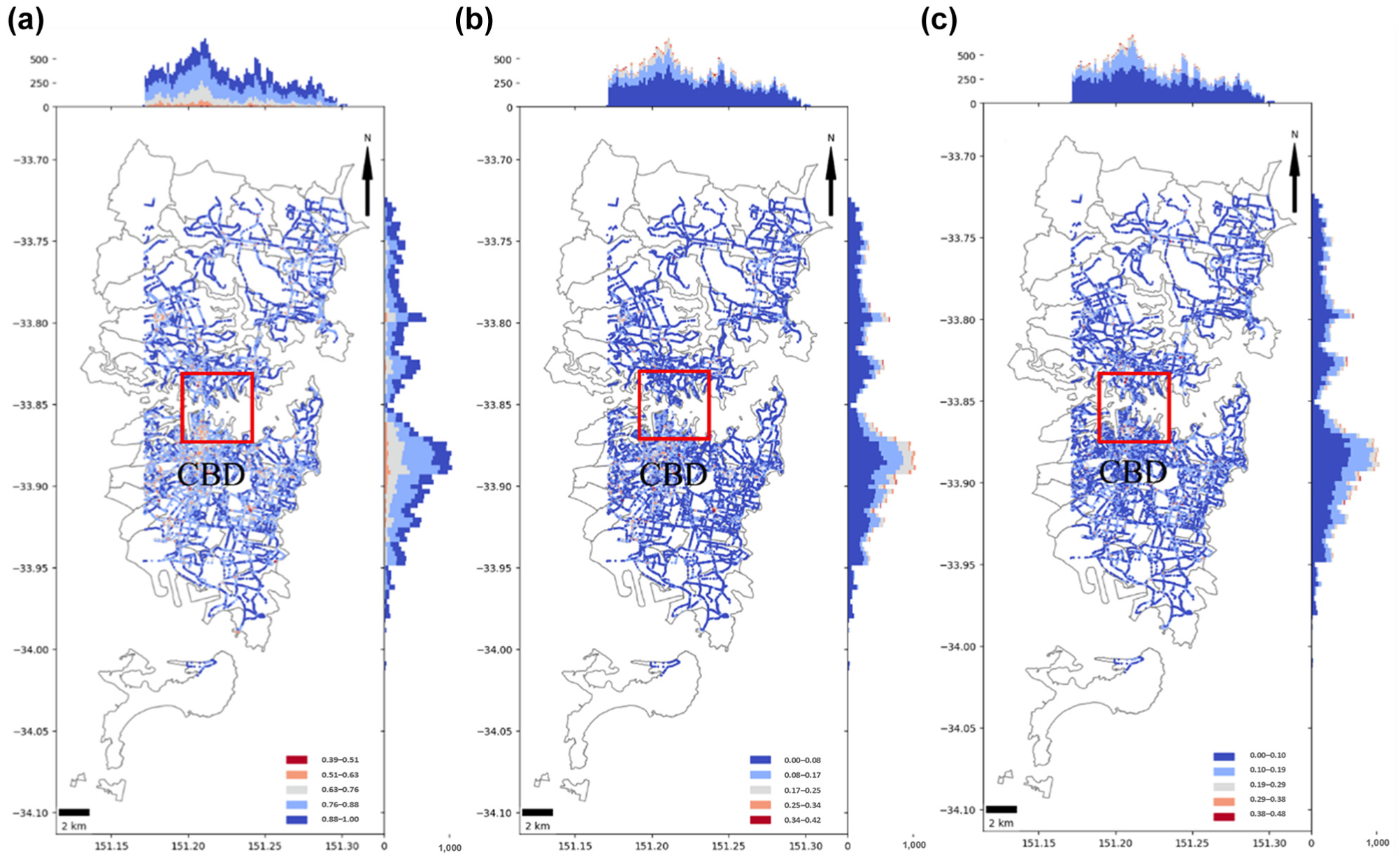
Spatial distribution and stacked histogram for resilience, vulnerability, and recoverability indices.
Resilience Metrics at the Zonal Level
The metrics at the point level were averaged for a zone to obtain the zonal metrics, such as the ZRI, ZVI, and ZReI. The descriptive statistics of these variables are given in Table 2. The average value of the ZRI for a zone was 0.84, indicating that 84% of the performance is retained within this zone. The minimum value of the ZRI was 0.75. The ZVI has a mean value of 0.07, indicating that, on average, a performance loss of only 7% occurs during the vulnerability phase. Similarly, for the ZReI, the average value was 0.09, indicating that, on average, there was only a 9% loss during the recoverability phase.
In addition, the geographical distribution of the ZRI, ZVI, and ZReI is shown in Figure 8. Zones in the southern portion of Sydney, Australia, are less resilient than the ones in the northern region, and the central zones are the least resilient. In addition, a less resilient zone is surrounded by another zone that has the same or slightly lower resilience level, indicating that some spatial autocorrelation may exist between the zones.
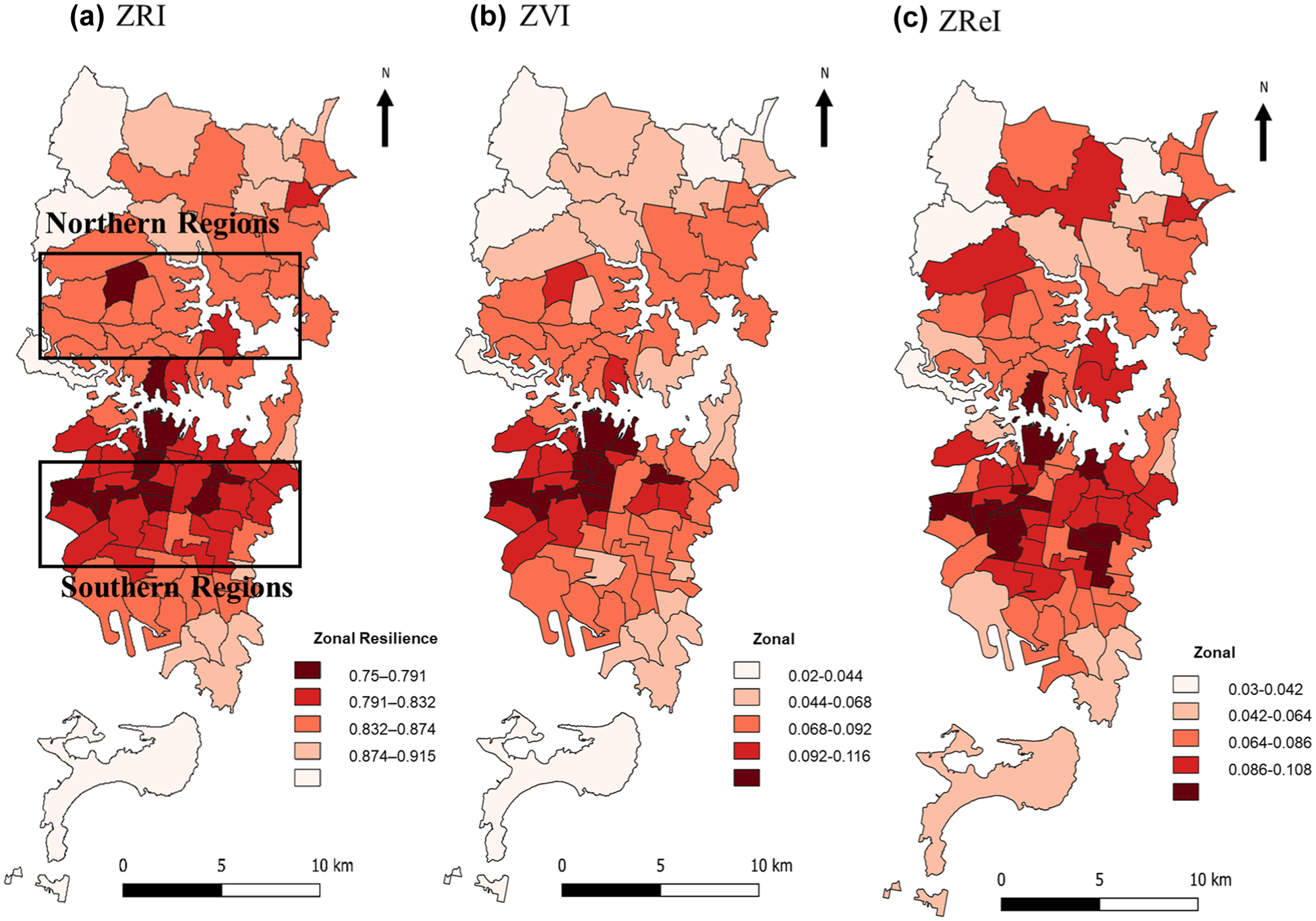
Spatial distribution of zonal resilience metrics.
Pearson Correlation
In this study, three dependent variables and 15 independent variables were considered. Understanding whether a linear relationship exists between these dependent and independent variables is essential. In addition, analyzing the correlation between the independent variables helps avoid multicollinearity in the model. The results of the correlation analysis are shown in Figure 9. The blank boxes indicate an insignificant correlation (p > 0.05), the bubble size indicates the strength, and the color indicates the sign of the correlation. The dependent variables in this study are ZRI, ZVI, and ZReI, and all other variables were considered independent. The analysis shows that the ZRI, ZVI, and ZReI strongly correlate with density measures, such as population density, ND, and bus stop density. Entropy measures, such as road category, LCE, and TE, correlate strongly with dependent variables. These measures strongly correlate with the ZRI, ZVI, and ZReI. When examining centrality measures, all show negative correlations with ZRI, with information centrality (IC) showing the strongest. The ZVI and ZReI show a strong correlation with IC. For the connectivity measures, only the average AC has a moderately strong correlation with the ZRI, ZVI, and ZReI.
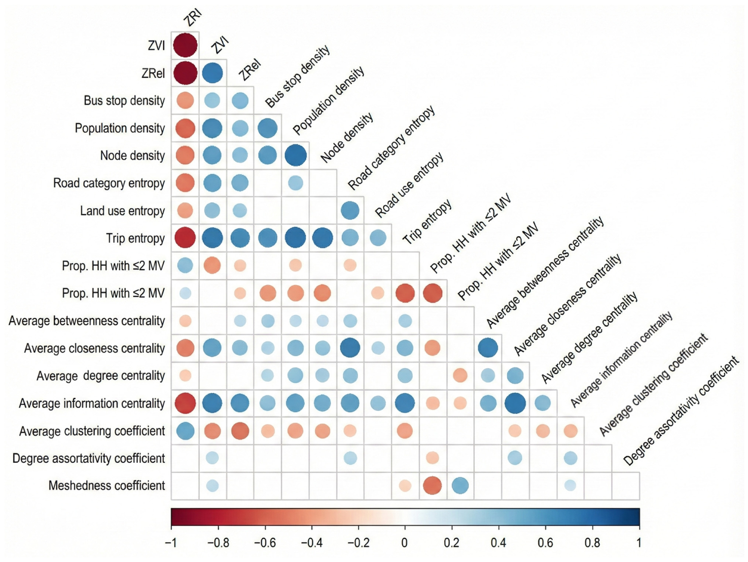
Correlogram of all variables.
Global Autocorrelation
Global autocorrelation refers to the similarity in spatial patterns for the variable of interest. It analyzes the degree to which similar values are close to each other. Global autocorrelation is commonly measured using Moran’s I statistic. The Moran’s I statistic can be calculated using Equation 9 where
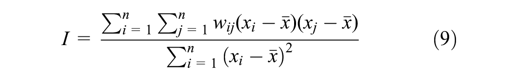
Moran’s I statistic was calculated using the Python package Exploratory Spatial Data Analysis (ESDA) ( 45 ). Moran’s I was calculated for the three dependent variables of ZRI, ZVI, and ZReI as 0.49, 0.54, and 0.3, respectively (all statistically significant). Therefore, while modeling, the effect of spatial autocorrelation must be considered because its presence violates the assumption of independence of observations. This violation would lead to the incorrect estimation of coefficients, because the effect of the surrounding units will not be considered during coefficient estimation. Therefore, in this study, the GWR model was estimated to quantify the impact of different independent variables on resilience indicators.
GWR Model
A GWR model was developed to account for the spatial autocorrelation in the dependent variable. Unlike a linear regression model, which considers a single coefficient for a variable, the GWR allows the coefficient to vary over space. The GWR model is represented by Equation 10.
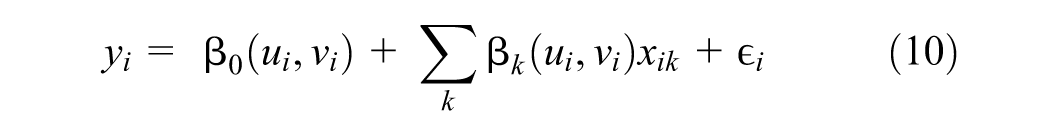
where
Geographically Weighted Regression Model of Zonal Resilience Index (ZRI), Zonal Vulnerability Index (ZVI), and Zonal Recoverability Index (ZReI)
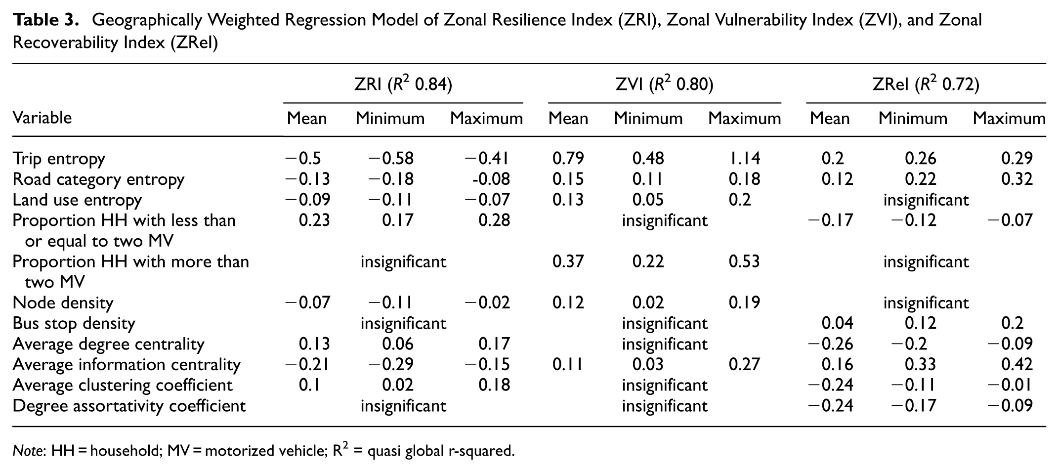
Note: HH = household; MV = motorized vehicle; R2 = quasi global r-squared.
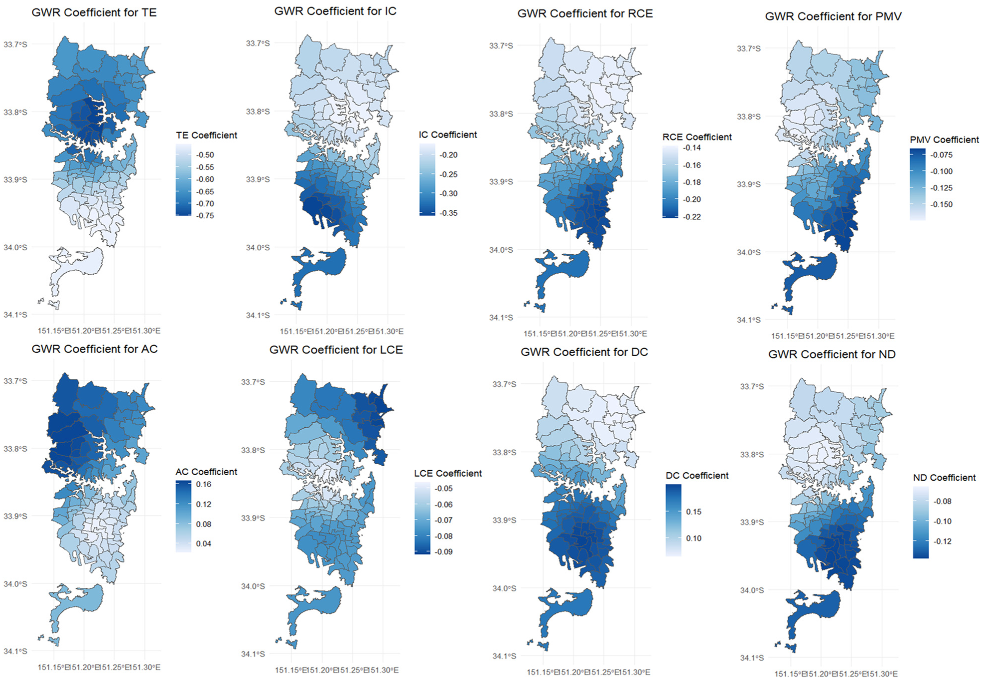
Geographically weighted regression model coefficients for zonal resilience index model.
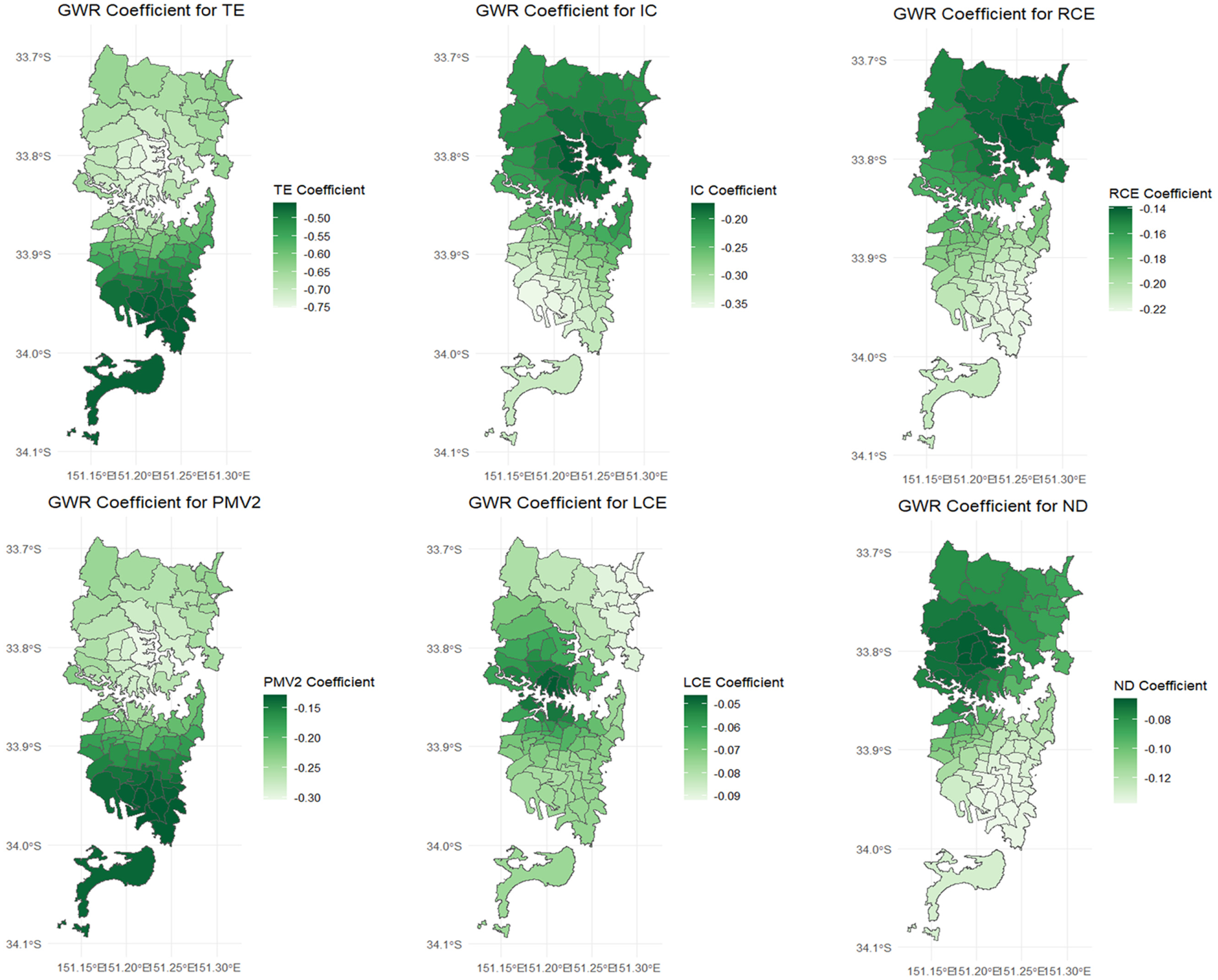
Geographically weighted regression model coefficients for ZVI model.
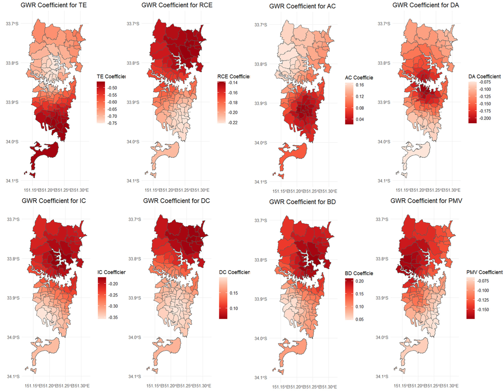
Geographically weighted regression model coefficients for zonal recoverability index model.
Road Category and Trip Heterogeneity
Examining the model results showed that the TE was significant across all three models. For the ZRI, its coefficients were from −0.58 to −0.41 (mean −0.50); for the ZVI, they were from 0.48 to 1.14 (mean 0.79); and for the ZReI, from 0.26 to 0.29 (mean 0.20). All results were statistically significant at p < 0.05. The other heterogeneity factor, RCE, was also significant in all models. For the ZRI, the coefficients were from −0.18 to −0.08 (mean −0.13); for the ZVI, from 0.11 to 0.18 (mean 0.15); and for the ZReI, from 0.22 to 0.32 (mean 0.12). All associations were statistically significant (p < 0.05). The LCE was significant only in the ZVI model, with coefficients from 0.05 to 0.20 (mean 0.13). It was not significant for the ZRI or ZReI.
Centrality
The DC was significant for the ZRI and ZReI. In the ZRI model, the coefficients were from 0.06 to 0.17 (mean 0.13); in the ZReI model, they were from −0.26 to −0.09 (mean −0.13). Both effects were statistically significant (p < 0.05). It was not significant for the ZVI. The IC was significant across all three metrics. For the ZRI, coefficients were from −0.29 to −0.15 (mean −0.21); for the ZVI, from 0.03 to 0.27 (mean 0.11); and for ZReI, from 0.33 to 0.42 (mean 0.16). All were significant at p < 0.05.
Connectivity
Only the average AC was significant for the ZRI and ZReI out of the four connectivity measures considered. For the ZRI, coefficients were from 0.02 to 0.18 (mean 0.10), and for the ZReI, from −0.24 to −0.01 (mean −0.11), both at p < 0.05. It was not significant for the ZVI. The DA was significant only for the ZReI, with coefficients from −0.24 to −0.09 (mean −0.17), statistically significant at p < 0.05. It was not significant in the ZRI or ZVI models. The ND was significant only for the ZVI, with coefficients from 0.02 to 0.19 (mean 0.12), significant at p < 0.05.
Bus Stop Density and Proportion of Motorized Vehicles
The proportion of households (HH) with ≤ 2 motorized vehicles (PMV) was significant for the ZRI and ZReI. For th ZRI, coefficients were from 0.17 to 0.28 (mean 0.23); for the ZReI, from −0.12 to −0.07 (mean −0.09); significant at p < 0.05. It was not significant for the ZVI. The proportion of HH with > 2 motorized vehicles (PMV2) was significant only in the ZVI model, with coefficients from 0.22 to 0.53 (mean 0.37), significant at p < 0.05. Bus stop density (BD) was significant only in the ZReI model, with coefficients from 0.04 to 0.12 (mean 0.04), p < 0.05. It was not significant for the ZRI or ZVI.
Model Validation
To ensure the robustness of the GWR model results, the model was validated using two approaches: (1) temporal validation using subset profiles from different parts of the month; and (2) spatial validation using alternative zone configurations. These checks help confirm whether the key relationships observed in the main model hold under different temporal and spatial conditions.
Splitting the Data Set into Subsets
To validate the model and ensure that the direction and influence of the variables remain consistent across different time periods, the data set was split into weekdays from June 1 to June 15 for the first part and weekdays from June 16 to June 30 for the second part. Average weekday profiles were developed for each data point in both parts, following the methodology outlined previously. Resilience metrics were then calculated at the point level and aggregated to the zonal level for each subset. These two subsets served as validation data sets, enabling the development of new models across different resilience metrics for comparison. Six models were developed to assess the consistency of the results. The model development results using both subsets of data are given in Tables 4 and 5.
Geographically Weighted Regression Model Validation Using Data Between June 1 and 15, 2018
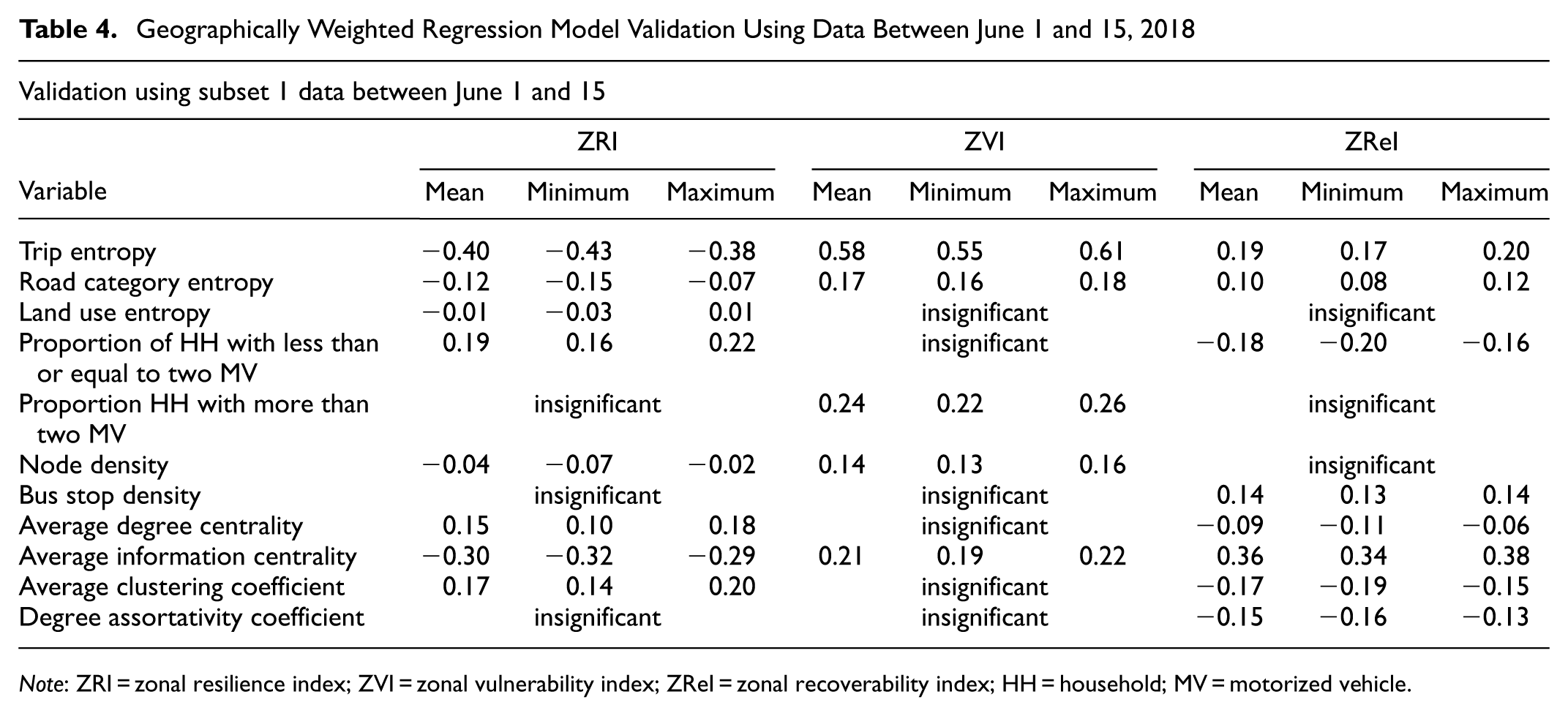
Note: ZRI = zonal resilience index; ZVI = zonal vulnerability index; ZReI = zonal recoverability index; HH = household; MV = motorized vehicle.
Geographically Weighted Regression Model Validation Using Data Between June 15 and 30, 2018
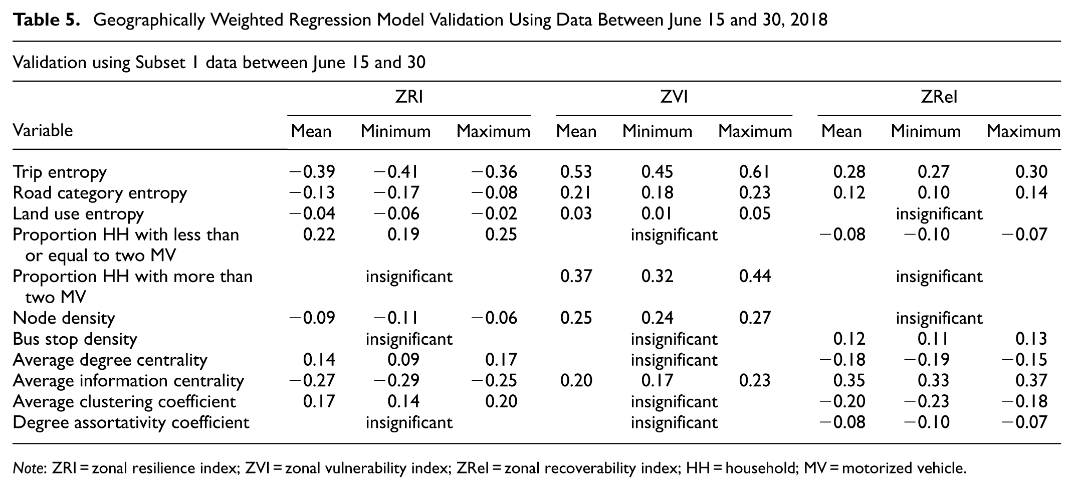
Note: ZRI = zonal resilience index; ZVI = zonal vulnerability index; ZReI = zonal recoverability index; HH = household; MV = motorized vehicle.
The results from the subset models indicated that the directionality of variables in the GWR model for the ZRI remained consistent with those presented in Table 3. In addition, the same variables were significant in both GWR models for the ZRI developed from Subsets 1 and 2. Similar observations were noted for the GWR model developed for the ZReI.
For the GWR model of the ZVI, developed using Subset 1 data, one variable—LCE—was insignificant, suggesting that the LCE does not significantly impact zonal vulnerability in this context. However, the same variable significantly affected the ZVI in the model using Subset 2 data. Of note, the direction of the effect for the remaining variables of ZVI remained consistent across both subsets.
This consistency in variable directionality and significance across subsets indicates that the GWR model effectively captures the stable spatial relationships between resilience metrics and explanatory variables, even with temporal variation in the data set. Therefore, the GWR model is suitable for this study because it reliably reflects the spatial variability in resilience factors across different periods.
Testing Variable Relationships Under Different Zone Sizes
To examine the effect of zone size on the relationship with independent variables, work started with the existing zone configuration of 82 zones. Different neighboring zones were merged for each new zone configuration to create larger ones. Figure 13 shows these different zone configurations derived from the original zones, and Table 6 details the IDs of the original zones that were merged (ID-1 and ID-2) along with the new IDs formed after merging. In addition, monthly average weekday data was utilized to develop these models.
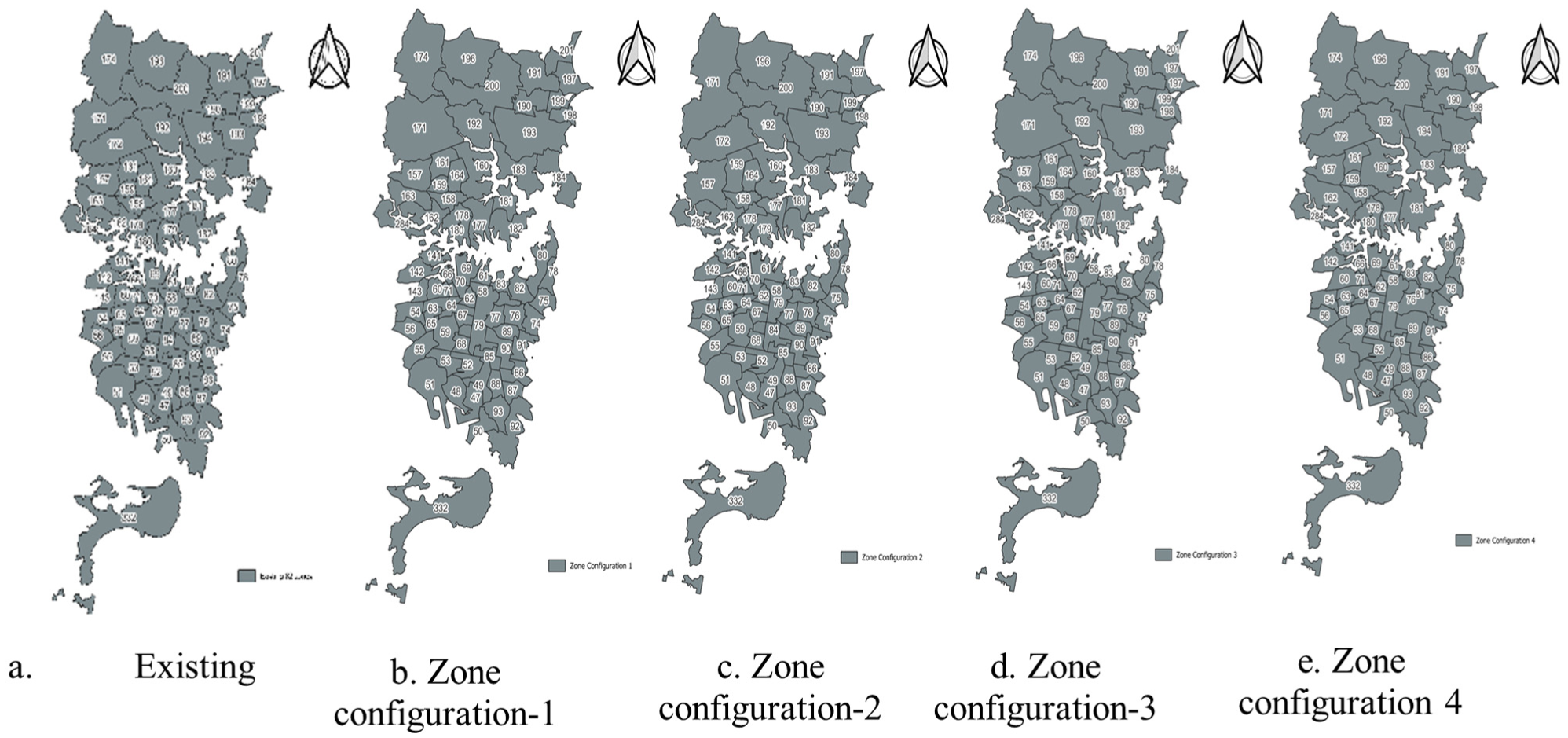
Different zone configurations.
Details of the Different Zones Merged and the New Zone ID .
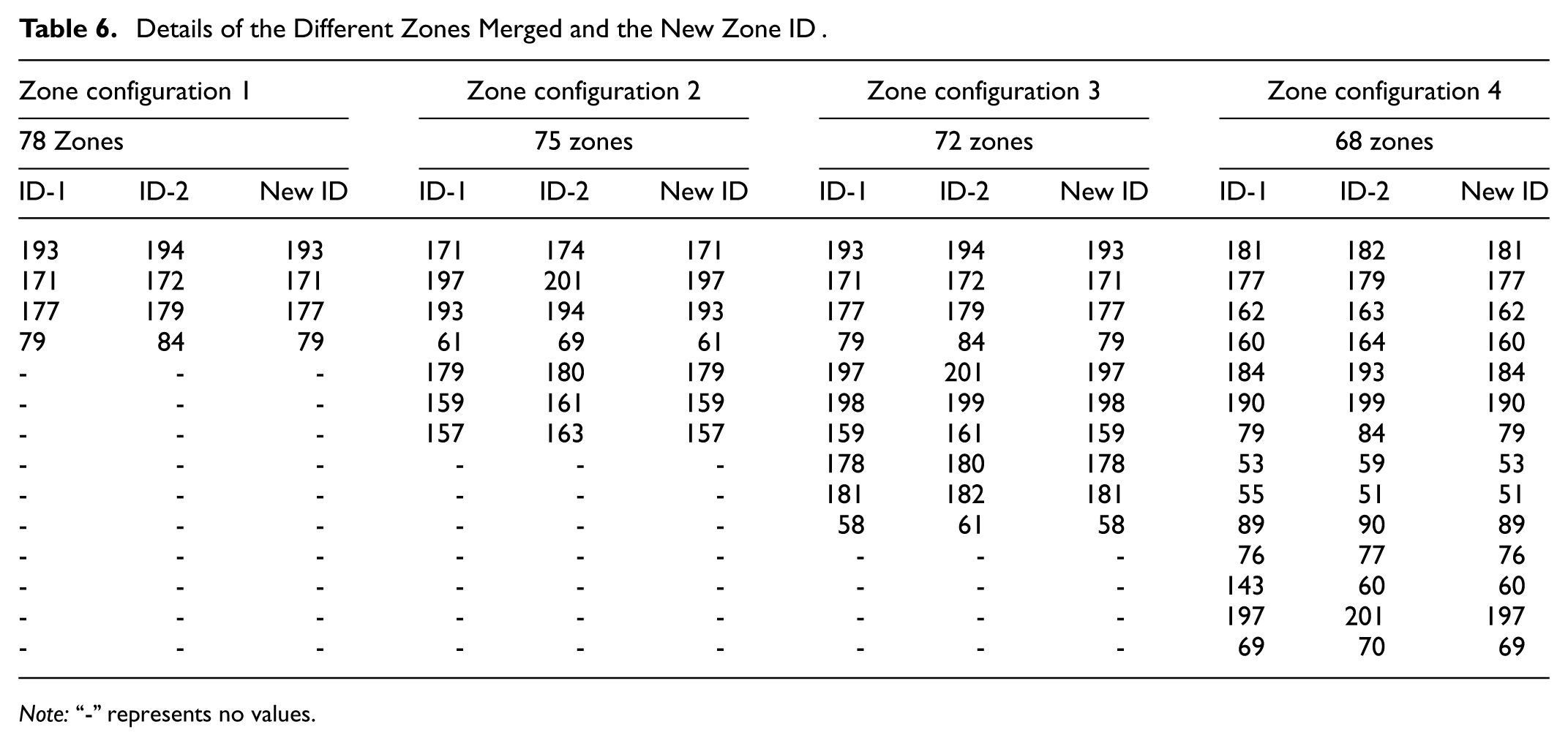
Note:“-” represents no values.
Of note, only zone merging was undertaken, as this approach simplified the calculation for merged zones. Splitting into new zones or creating grid-based zones would have introduced complexity into the variable calculations and required numerous assumptions. To avoid these complications, existing zones were merged to form larger zones. These different zone configurations and their respective variables were then used to develop new GWR models, with the results presented in Tables 7–11.
Geographically Weighted Regression Model for Existing Configuration of 82 Zones
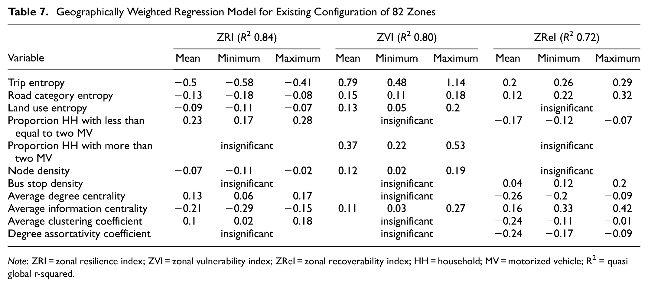
Note: ZRI = zonal resilience index; ZVI = zonal vulnerability index; ZReI = zonal recoverability index; HH = household; MV = motorized vehicle; R2 = quasi global r-squared.
Geographically Weighted Regression Model for Zone Configuration 1
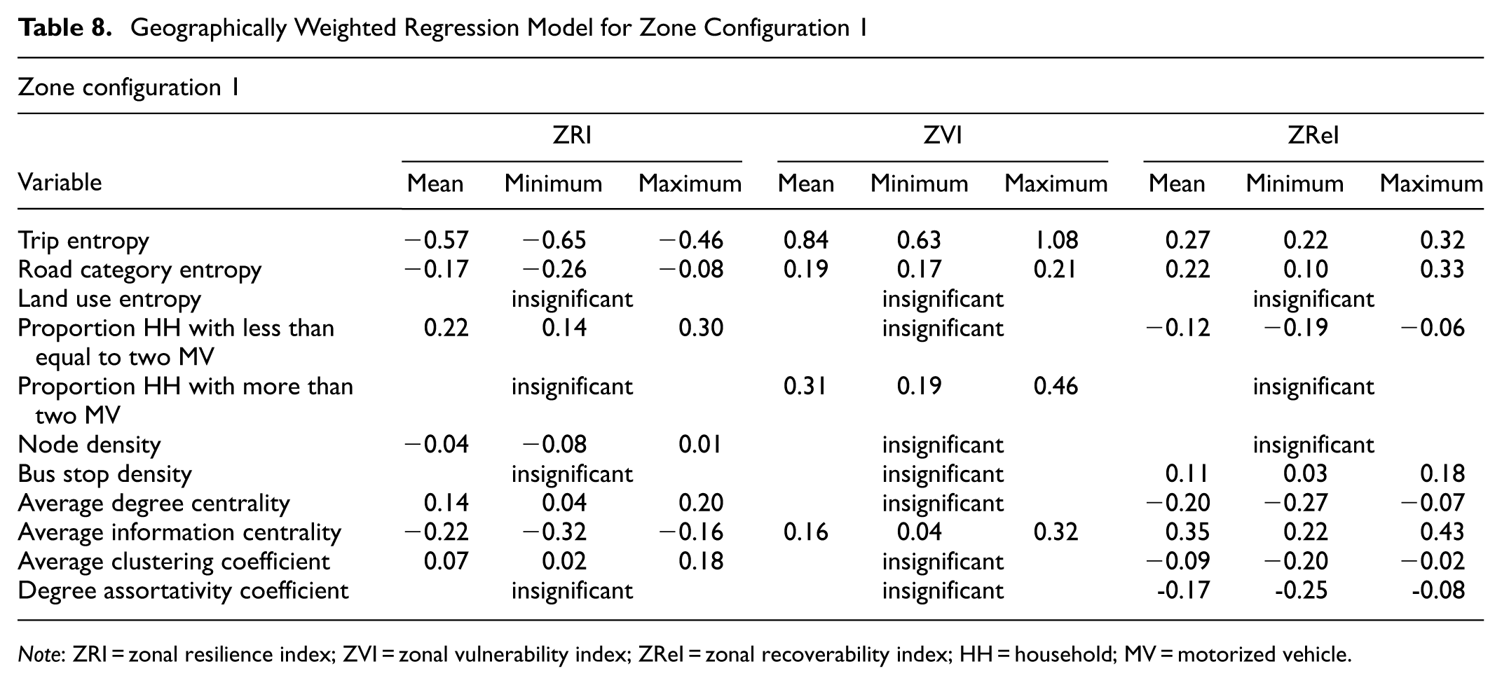
Note: ZRI = zonal resilience index; ZVI = zonal vulnerability index; ZReI = zonal recoverability index; HH = household; MV = motorized vehicle.
Geographically Weighted Regression Model for Zone Configuration 2
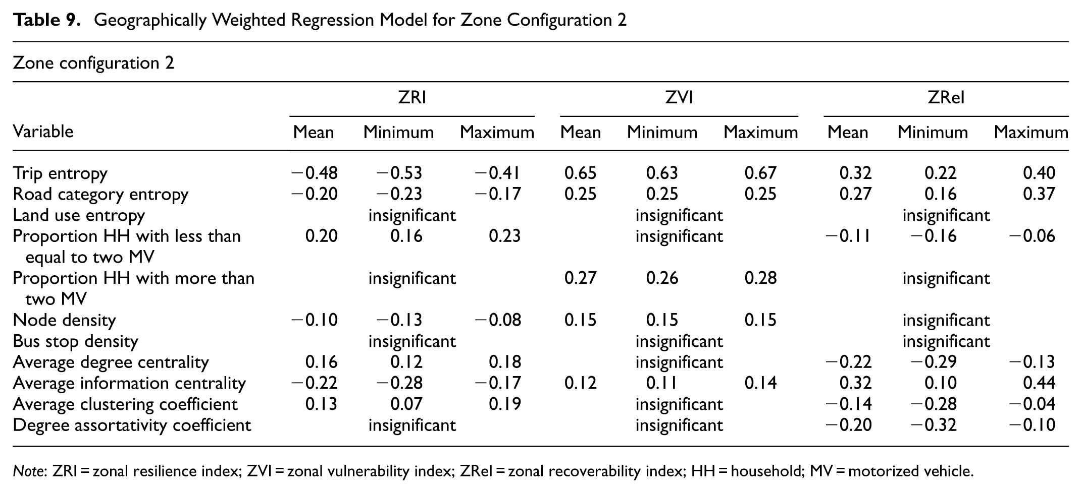
Note: ZRI = zonal resilience index; ZVI = zonal vulnerability index; ZReI = zonal recoverability index; HH = household; MV = motorized vehicle.
Geographically Weighted Regression Model for Zone Configuration 3
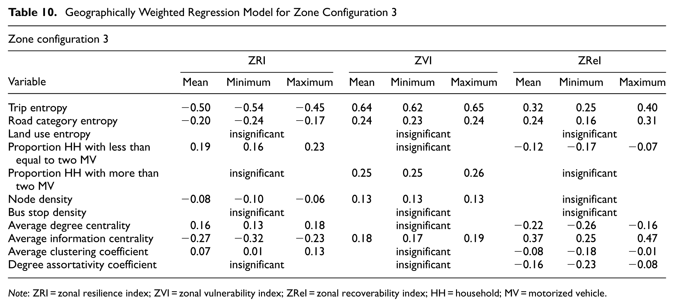
Note: ZRI = zonal resilience index; ZVI = zonal vulnerability index; ZReI = zonal recoverability index; HH = household; MV = motorized vehicle.
Geographically Weighted Regression Model for Zone Configuration 4
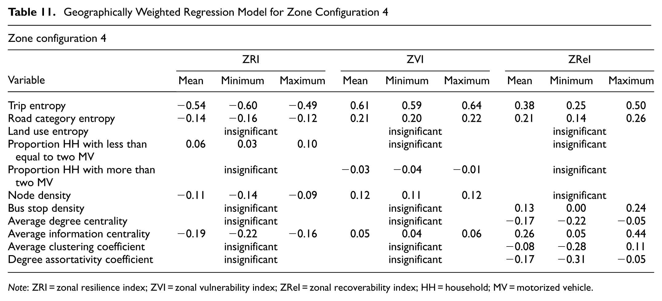
Note: ZRI = zonal resilience index; ZVI = zonal vulnerability index; ZReI = zonal recoverability index; HH = household; MV = motorized vehicle.
The results from the different zone configurations show that changes in zone sizes make the effect of certain variables insignificant. However, the direction of relationships remained largely consistent across most models, with only one exception. In the ZVI model of zone configuration 4 (68 zones), the effect of the variable PMV2 was reversed compared with the results given in Table 7 for the original configuration of 82 zones. This may be because of merging zones with different characteristics, which can average out or hide local patterns. This issue is related to the modifiable areal unit problem (MAUP), where results can change depending on how the zones are defined.
Another observation was that the variable LCE was consistently insignificant in all models for each zone configuration, suggesting that its effects may only manifest at finer spatial resolutions. This result indicates that land use does not significantly influence resilience or its components under these alternative configurations, contrasting with the observed results for the original 82-zone model. These findings suggest that future research should explore how to define zones more effectively, possibly using regular grids or grouping zones with similar characteristics to improve the accuracy and usefulness of resilience modeling.
In addition, merging zones generally led to slight shifts in the mean values of the coefficients; however, the direction and significance of most variables remained stable across configurations. These findings suggest that while certain indicators are robust to changes in zone configuration, others, such as the LCE, may be more sensitive to spatial aggregation. This highlights the importance of carefully considering zone size in resilience modeling and interpreting results.
Discussion and Policy Implications
This section explains the results from the GWR model and discusses how they can be helpful in planning and policy. It focuses on the main variables found significant and presents what they mean for managing road network performance under regular day-to-day traffic disruptions.
Road Category and Trip Heterogeneity
The TE and RCE reduced resilience and significantly increased vulnerability and recovery losses. These variables represent the variation in travel modes and road types within a zone. A higher TE means a zone has a more mixed-use of cars, motorbikes, buses, and non-motorized modes. The RCE captures the mix of different road types, such as motorways, arterials, and residential streets.
The consistent effect of the TE across all three models suggests that zones with higher mode-based heterogeneity experience more complex traffic interactions. As the variety of travel modes increases, so do differences in speeds, stopping behavior, and road space usage. This leads to irregular flow patterns, which reduce the system’s ability to absorb and recover from routine congestion. For instance, interactions between buses and two-wheelers or between cars and non-motorized users may cause disruptions at intersections or during lane changes.
The effect of the RCE can be attributed to the speed reduction caused by the movement of vehicles from one road category to another, leading to forced speed reduction. The more heterogeneous a zone is, the more frequent the speed change of the vehicles will be, and the greater the performance loss will be. For instance, a vehicle moving from a highway to a local street will experience a significant drop in speed, disrupting traffic flow and reducing overall network efficiency. The frequent transitions between road categories in a zone with high entropy can lead to more stop-and-go driving patterns, longer travel times, and increased congestion, all contributing to performance loss during the vulnerability and recovery phases.
For LCE, different land uses in a zone lead to higher performance losses. This is because different activities create complex interactions between road users, such as pedestrians and vehicles, causing frequent stops and longer signal delays, further disrupting traffic flow and increasing performance loss. However, it is important to note that this analysis is based on car speed data. Therefore, any land use planning decisions should also consider the needs and performance of other road users, such as pedestrians, cyclists, and public transport users, to ensure a balanced and inclusive approach.
The previous results could be used to make informed policy decisions. For example, dedicated lanes for buses or two-wheelers can help reduce conflicts in zones with high TEs. Smoother transitions between road categories through clearer road hierarchy planning and signal coordination can reduce speed shifts and instability. Mixed-use zones should be designed with buffers, channelized pedestrian crossings, and turn restrictions to minimize interruptions during peak hours.
Centrality
Only the DC and IC were significant from the four centrality measures used in model building. Betweenness centrality and closeness centrality measures impacted resilience significantly in previous studies ( 19 , 22 ) at the link level; these metrics were not significant in our zonal-level analysis. One possible explanation is that these centrality measures are highly sensitive to individual link positions within the global network. When aggregated at the zone level, their localized influence may be averaged out, especially in zones with diverse street structures or where centrality values vary widely across internal nodes. This suggests that while betweenness and closeness centrality are valuable indicators at finer spatial scales, they may not be as effective in explaining resilience patterns when measured at coarser (zonal) levels.
The average DC had a significant positive effect on resilience and improved the recoverability of a zone, indicating that a higher DC in a zone results in lower performance loss. This can be related to the efficient dispersion of traffic to the connected intersections and allowing for quick recovery. In zones with a high DC, traffic can be rerouted or dispersed more effectively when a disruption occurs, reducing the likelihood of congestion and allowing for quicker recovery. In addition, the results of the DC were similar to those of the Niu et al. ( 19 ) model for the resilience triangle area, where the resilience increased with an increase in DC. Another significant centrality measure, based on the model results in this study, is IC. A zone with a high IC attracts a large amount of traffic because it contains critical nodes. However, this increased vehicular flow can lead to higher performance loss as these critical nodes become potential bottlenecks.
These results could be used to enhance local intersection connectivity in low-degree zones and improve resilience. For zones with a high IC, preemptive measures, such as adaptive signal plans, incident response strategies, and even minor geometric improvements (e.g., turning lanes or bypasses) can prevent bottlenecks. These areas may also require special operational control during planned events or emergencies.
Connectivity
The AC was positively linked to resilience and negatively to recovery loss. A zone with a high AC indicates that its nodes are connected, allowing for efficient flow dispersion to the other intersections and low-performance loss for those zones. This interconnectedness allows traffic to redistribute more effectively, reducing congestion and aiding in quicker recovery after disruptions.
In addition, the DA improved recovery, suggesting that zones with similar-capacity intersections connected can handle traffic more efficiently. The DA coefficient measures the connectivity of nodes with the same degree. A higher DA coefficient indicates that the same type of nodes are connected. A higher DA coefficient would indicate a more efficient dispersion of vehicular flow from the intersection, avoiding the creation of blockades at the intersection, as same-capacity intersections are connected. For example, traffic can be distributed more evenly and efficiently in a road network where intersections (nodes) with a high degree (many connecting roads) are primarily connected to other high degree intersections. This prevents bottlenecks, as these well-connected intersections can handle higher traffic volumes and reduce congestion by allowing for smooth dispersion. However, assume an example where a node with a lower degree (e.g., three degrees) is connected to a node with four degrees or more. In that case, the traffic flow from a higher degree node may lead to traffic buildup in a lower degree node, and the queue may eventually spill back to a higher degree node, leading to longer recovery times and, therefore, a higher performance loss during recovery. The results of the DA coefficient improving the resilience match the observations made by Buhl et al. ( 42 ), where the DA coefficient had a positive correlation with the robustness of the network subjected to random node removal.
The ND had a positive association with vulnerability. This could possibly be because of more frequent stops, leading to longer queues and slow vehicular movement and increased losses during the vulnerability and recoverability phase.
Planning policies should encourage internally well-connected layouts, such as grid-like patterns, but avoid excessive ND. Where the ND is already high, vehicle movement can be supported by simplifying intersection control, managing pedestrian crossings, and restricting side-road access during peak times. Road network upgrades in low-clustering zones should aim to close loops and create alternate intra-zonal paths. For long-term resilience, assortativity can be improved by aligning the functional class of connected roads.
Public Transport and Motorization
Bus stop density had a clear negative effect on recovery. High bus stop frequency, especially where buses stop on the main carriageway, may delay other traffic and slow the system’s return to normal speeds. Public transport is essential; unmanaged stops can reduce network efficiency.
Zones with higher household motorization (PMV2) showed greater vulnerability; however, zones with fewer vehicles were more resilient and recovered faster. Higher motorization probably increases traffic demand, which can easily overwhelm the available capacity during disruptions.
The planners could reduce performance loss by reducing car dependency in highly motorized zones using demand management, such as restricted parking, vehicle quotas, or road pricing. Public transport services should be supported by infrastructure upgrades, including off-street bus bays, optimized stop spacing, and transit signal priority. In busy corridors, especially with narrow roads, consolidation of bus stops or rerouting may be needed to avoid recovery delays.
Conclusion
Road networks play a vital role in economic growth; however, they often get stressed because of travel demand fluctuations, traffic incidents, road maintenance, and other factors. This leads to increased delays, emergency response times, and fuel consumption. This paper uses the resilience triangle approach to evaluate performance loss because of travel demand or fluctuating traffic flow. The resilience-based approach divides the performance loss into vulnerability and recoverability, allowing us to understand the congestion dynamics.
Various factors, such as demographics, socioeconomic conditions, land use, and road network structure, can influence the vulnerability or recoverability of a road network. Previous studies have not extensively examined the effect of travel demand fluctuations from a resilience perspective or the influence of different factors. This study focuses on applying the concept of resilience to understand performance loss because of travel demand fluctuations and identifies factors affecting the city of Sydney.
This study was conducted at a zonal level using Google Maps speed data. Three metrics, ZRI, ZVI and ZReI, were developed to study overall resilience, vulnerability and recoverability. Since the data had spatial properties, the authors hypothesized that spatial autocorrelation exists. This was confirmed by the results of Moran’s I statistics. Therefore, three GWR models were developed to understand the effect of variables on resilience metrics while accounting for spatial autocorrelation.
The results from the model showed that out of 15 variables, 10 significantly affected resilience or its components. The heterogeneity-based variables, such as LCE, RCE, and TE, affected resilience negatively and further increased performance loss. This indicates that any heterogeneity in a zone leads to performance loss. In addition, centrality measures influence the resilience of a zone. For example, a zone with a high IC has low resilience because it contains central nodes. The connectivity measures, such as the AC and DA coefficients, show that a zone with high connectivity among nodes of the same degree supports better resilience by enabling efficient traffic dispersion. Furthermore, the variable related to MV ownership indicated that lower motorization in a zone would improve its resilience.
The results of the model have been further validated by developing two models using the subset of the data and five different models by checking the effect of different zone sizes on the independent variable relations. The results showed that most of the variables considered were statistically significant despite different zone sizes and subsets. However, certain variables become insignificant with a change in zone size. This highlights the importance of carefully considering zone size in resilience modeling and interpreting results.
This study provides an understanding of performance loss from the perspective of resilience. In addition, it details what factors can affect the performance losses and the nature of their impact. Policymakers could utilize these insights to create policies for individual zones. The results can be helpful in zonal congestion pricing by basing the road pricing on the value of zonal resilience. The effect of land use distribution on zonal resilience can help the planning authorities decide the land use mix for the developing towns. The effect of network structure on zonal resilience can help select a road network layout that reduces interruptions to traffic. The selection of safe zones for evacuation planning can be based on zonal resilience.
The proposed methodology produced consistent results across different subsets and zone configurations; three key limitations should be acknowledged. First, this study used speed data for a single month (June 2018), which may not capture seasonal variations in travel patterns. Although average weekday profiles helped generalize typical behavior, incorporating data from multiple months or seasons could improve the robustness of findings. Second, some variables showed sensitivity to zone configuration, highlighting the MAUP, a known issue where results vary depending on the spatial unit used. Future studies should explore alternative zoning methods and year-round data sets to enhance the generalizability and policy relevance of resilience modeling. Third, the speed data was collected using the Google Maps Speed API, which has since been deprecated. This limits the ability to reproduce the same data set and raises the possibility that certain zones or road categories may have had uneven data coverage. Future studies should explore alternative zoning methods and year-round data sets and compare multiple data sources, such as TomTom, HERE, INRIX, or other crowdsource data sets, to improve the reliability and generalizability of resilience modeling.
Footnotes
Acknowledgements
The authors thank Dr. Vinayak Dixit, Professor at the University of New South Wales, for sharing the raw speed data.
Author Contributions
The authors confirm contribution to the paper as follows: conceptulization: S. Chand; data curation: P. Lalwani; formal analysis: P. Lalwani; funding acquisition: S. Chand; investigation: P. Lalwani; methodology: P. Lalwani, S. Chand; supervision: S. Chand; project administration: S. Chand; resources: S. Chand; visualization: P. Lalwani; writing of original draft: P. Lalwani; writing review and editing: P. Lalwani, S. Chand; All authors reviewed the results and approved the final version of the manuscript.
Declaration of Conflicting Interests
The authors declared no potential conflicts of interest with respect to the research, authorship, and/or publication of this article.
Funding
The authors disclosed receipt of the following financial support for the research, authorship, and/or publication of this article: The authors would like to thank the Science and Engineering Research Board for supporting this project under grant SRG/2023/001358 “Quantifying and comparing road network resilience of Indian cities using crowdsourced data and simulation”.