
Abstract
Transit service reliability is important for transit planning and operations as well as passenger experience. Large travel time variations increase operating costs and negatively affect passenger satisfaction. Existing literature focuses on specific aspects of transit travel times but less on how these aspects interact with each other. This paper proposes to combine previous research efforts by further decomposing observed trip travel times into four elements using 3 months of archived vehicle location and fare transaction data. Departure times and inter-stop travel times are obtained from vehicle locations. Dwell times at stops are estimated from fare transaction data using a dwell time model. Red-light waiting times are calculated using the vehicle locations and estimated signal timing plans. Then, using these as inputs, we identify important trip elements affecting the overall travel time variation, as well as how much variation can be attributed to each trip element using variance-based and one-at-a-time sensitivity analyses. The overall travel times and red-light waiting times are more affected by interaction effects between trip elements, whereas the overall inter-stop times and dwell times are mainly affected by large individual variations. The results suggest that planners must consider potential chain reactions where small variations in one trip element can lead to significant changes in the overall trip times as a result of interaction effects with varying cycle lengths in fixed signal timing plans. These findings will help planners better integrate available data sets, carry out comprehensive analyses, and pinpoint the determinants affecting travel time variation on each route.
Reliable travel time is important for both transit agency operations and passenger satisfaction. Transit agencies and planners have been striving to achieve better reliability. From the agencies’ perspective, travel time reliability affects both vehicle and operator scheduling. Transit planners typically add schedule padding or layover times to account for potential travel time variations, which will, unfortunately, increase the operating costs ( 1 ). Missing a layover will also propagate delays to downstream trips and cause driver dissatisfaction issues ( 1 ). Unreliable travel times will also force passengers to budget additional time to arrive at their destination on time, which in turn affects their satisfaction and mode choice ( 2 ). Some passengers value reliable service more than service frequency and faster travel times ( 3 , 4 ).
Many studies have looked at the reliability of transit travel times from specific perspectives, such as travel times on various analysis levels (e.g., timepoint to timepoint) ( 5 ), dwell times at stops ( 6 ), as well as signal priority measures at intersections ( 7 ). However, little attention has been paid to how these different elements interact with each other. For example, given signal synchronization, if the vehicle always arrives at the stop during the red light, dwell time variation may become less critical. On the other hand, if the vehicle always arrives during the green light, the previous inter-stop traffic and dwell time can become more critical when the driver tries to cross the intersection before the light turns red. Thus, it is still important to consider the interactions between different trip elements as well as to quantify the sensitivity of each trip element.
We hope, therefore, to better integrate various data sources already available to most agencies, such as vehicle position and fare collection data. Then, we aim to carry out a more detailed comprehensive analysis that would include all these various aspects to better describe these factors affecting transit travel time variations. Finally, we also attempt to help planners better identify the important determinants affecting travel time variation among these factors on each route, which will help create specific strategies to improve travel time reliability.
This paper aims to combine the previous research efforts, further decomposing the travel times by splitting the overall travel times into various trip elements. We will then conduct a sensitivity analysis using variance-based sensitivity analysis and one-at-a-time analysis. This would allow us to answer the two questions: Where do travel time variations come from? How much travel time variation can be attributed to each trip element, that is, departure time, inter-stop time, ridership change, and traffic signal timing change?
We propose to answer these two questions by further decomposing observed trip travel times using 3 months of archived transit data from various sources in Montréal, Canada. The existing literature focuses on three aspects of total travel time: inter-stop time (congestion), dwell time (ridership), and red light waiting times (traffic signals). The inter-stop times, that is, how long the vehicle traveled from one stop to another, are easy to obtain from the vehicle location system. Unfortunately, because of data availability issues, we will create two models to estimate dwell times and red-light waiting times. The dwell time, that is, how long the vehicle is stationary for passenger activities at a given stop, is estimated based on the ridership observations, where we used 25,000 on-board observations to estimate a dwell time model, and the model is applied to the ridership data obtained from automated fare collection where there are no on-board observations. Red-light waiting times, on the other hand, are the interaction between the vehicle arrival times at the signal and the signal timing plan, which we will have to calculate separately. The arrival time can be calculated using the departure time plus the travel time up to the given intersection. The traffic signal timing plans, including the timing plan changes, offset, red length, and cycle length, are estimated based on the vehicle location observations using the methodology proposed by Fayazi et al. ( 8 ). Since traffic signal timings are not under the agency’s control, we treat them as a fixed input and analyze the variations in red-light waiting times as a result.
Finally, we conduct two sensitivity analyses on these decomposed times to demonstrate the importance of each trip element. First, we propose using the variance-based analysis, followed by the one-at-a-time analysis. The variance-based analysis is a global method that can handle interaction effects and non-linearity among different variables ( 9 ). The results provide two indices with regard to the proportion of variation that can be attributed to each trip element, one with the interaction effects and one without. We also perform some example one-at-a-time analyses to demonstrate the non-linearity observed between the variation of a trip element and the overall variation in trip travel times.
The results will enhance our understanding of travel time variations and help planners identify certain locations or trip elements affecting travel time variations. In turn, these insights could help agencies target specific issues, choose the appropriate strategy to improve the reliability of a given route, develop more robust transit schedules, and thus improve passenger experiences.
This paper is structured as follows. We will summarize existing research contexts in the literature review section. We will then explain the research framework, data sources, and detailed methodology in the methodology and data section. Next, we will show the result of our case study using data from Montréal, Canada in the case study section. Finally, in the conclusions and future research section, we summarize our work and results from this paper, as well as showing potential future expansions to this work.
Literature Review
Transit reliability measures are commonly used by transit agencies in their planning and operations. Academics have also studied specific elements of transit reliability and proposed numerous additional measures. The focus of current literature is typically on different levels of travel time variations, ridership variations which relate to dwell times, and transit priority measures.
Research has focused extensively on transit travel times since the implementation of automated vehicle location systems. Travel time variations are important for transit agencies because they serve as a key scheduling input to determine the schedule padding and layover times needed, which affect vehicle requirements ( 10 ). The variations are typically analyzed at four different levels: line, trip, timepoint to timepoint, and stop-to-stop levels according to an agency survey ( 1 ). The analyses for travel time variations have focused on typical variation measures such as the standard deviation, coefficient of variation, or a predefined percentile ( 10 ).
Common factors affecting transit travel times are typically route length, passenger activity, and number of signalized intersections, dating back to 1984 from Abkowitz and Engelstein ( 11 ). Researchers also show that the number of stops, direction, time of the day, dwell time, and weather variations also have significant effects on route run time ( 12 ).
Some researchers have also observed mixture travel time distributions in recent years ( 13 , 14 ). A mixture distribution means travel time observations are generated first from a collection of underlying distributions or operating conditions (e.g., free-flow versus congested traffic flows) with various associated probabilities ( 13 ). The value is then selected from the selected probability distribution. Travel times following the mixture distribution means that if we put the observed travel times in a histogram, we can observe more than one peak, unlike the normal distribution or a skewed distribution with one single peak.
Figure 1 shows an example of a mixture distribution with multiple peaks in the distribution shape observed on the westbound Route 27 departing at 6:30 am in Montréal. In the figure, we can observe three main peaks at roughly 6:46:30, 6:48:00, and 6:49:30, and many smaller peaks earlier and after the three main peaks. Each peak, separated by roughly 1 min and 30 s, would represent an underlying distribution or operating condition. Given that the traffic signal cycle lengths for the last stretch of this route are 90 s, we would hypothesize that it relates to whether the bus misses a traffic signal cycle or not.
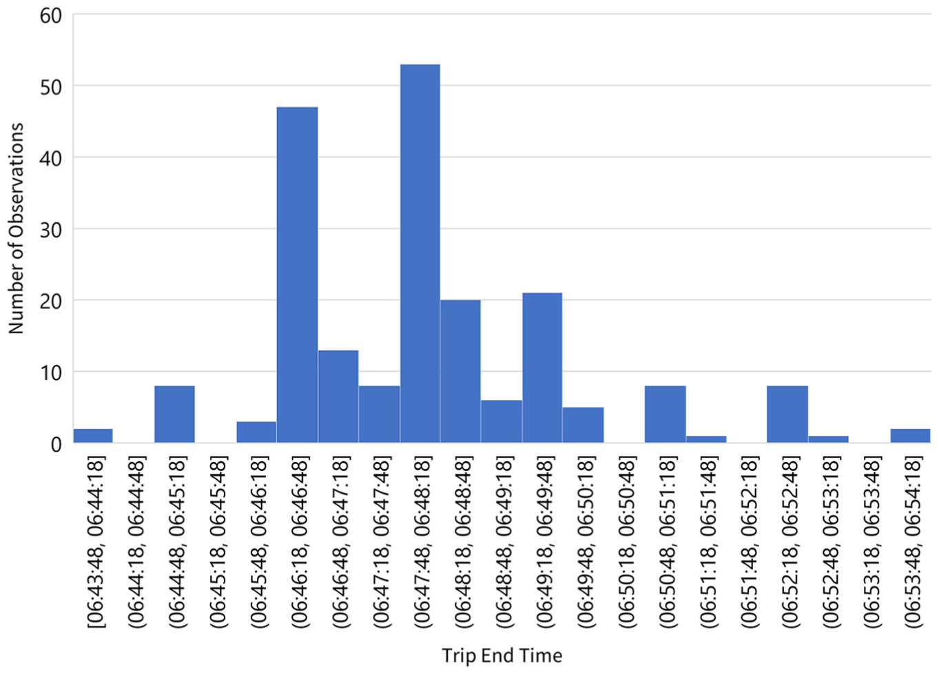
Example of mixture travel time distribution observed for trips departing at 6:30 on westbound Route 27 in Montréal.
In addition, even the smallest scale so far, namely the stop-to-stop scale, consists of the travel time between the two stops, dwell time at one stop, and potentially multiple traffic signal waiting times. Buses routinely wait for traffic signals, and higher ridership at a stop could also contribute to buses missing a green light. A much finer analysis scale with the ability to better isolate various trip elements and handle interaction effects among these elements is needed to attribute the travel time variation to a specific issue or a combination of issues.
Dwell times have also received high coverage in previous studies. It is defined as the time a vehicle spends at stops for passenger boarding and alighting, typically the time between the door opening and closing ( 10 ). Similar to travel time studies, dwell time studies have also focused on typical variation measures such as the standard deviation, coefficient of variation, or a predefined percentile ( 10 ). Some studies have analyzed stop-level dwell times, which can be compared with vehicle load to understand the source of dwell time variability. The variability could be a result of passenger boarding and alighting activities, existing crowding in vehicles which makes boarding and alighting difficult, fare payment methods, and ramp usages ( 6 , 15 , 16 ). However, there is less attention in the existing literature on how dwell times might affect the overall travel times.
The Transit Capacity and Quality of Service Manual ( 10 ) does not consider the time a vehicle remains stationary at the stops after passenger boardings and alightings as dwell time, such as red-light waiting time. Most traffic signal–related studies in the transit context are related to transit signal priorities for transit vehicles. Many studies show positive impacts of transit priority signals on reducing transit travel times ( 17 ). However, some other studies failed to show any significant travel time gains from signal priority, and they speculated that the no right turn on red policy combined with near-side stops hinders bus departures ( 18 ). In addition, many previous studies only considered the number of priority signals in the model and didn’t include any detailed signal timing information that could have contributed to the situation.
For some cities, especially in downtown areas, the majority of the signalized intersections still use a fixed timing plan. Researchers have suggested that good arrival time predictions are important in these cities for transit priority signals to be effective at reducing travel times ( 19 ). Better inter-stop and dwell time estimations are needed to improve the arrival time predictions. Scheduling strategies can also be adapted to take advantage of transit priority signals ( 20 ). However, these previous studies have tended to focus on one specific intersection or a few consecutive intersections on a given corridor, which would have similar base timings. Similarly, some studies only included the number of priority signals to model their effects, which essentially assumes these signals behave similarly. Since buses can make turns and travel through multiple corridors, the signal synchronization and cycle lengths may all be different in reality. Smaller intersections typically have shorter cycle lengths, while large intersections have longer cycle lengths. There is still a need to consider how the travel time and red-light waiting times are affected by varying signal cycle lengths and synchronization patterns.
Overall, the literature has mostly focused on the travel time impacts from one specific element of the transit system, namely the variation in travel times, dwell times, and signal priorities. There is still less attention on combining these various elements to examine how these travel time elements affect and interact with each other. For example, given a signal synchronization, if the vehicle always arrives at the stop during the red light, dwell time variation can become less critical since the bus is stopped by the signal anyway. On the other hand, if the vehicle always arrives during the green light, the previous inter-stop traffic and dwell time can become more critical when the bus tries to rush through the intersection before the light turns red.
In addition, since transit agencies have limited resources there is still a need to help planners prioritize their resources. It is thus important to determine which trip element is more important on a given route to reduce the overall travel time variations. By evaluating the importance of each trip element, planners can select a good and effective strategy to improve the reliability of a specific route.
Thus, in this paper, we propose a framework to further decompose transit travel times so that the variation of each trip element along the route can be isolated. Given the limitations of earlier studies, we also conduct a sensitivity analysis to rank the importance of each trip element based on its potential impact on the overall travel times. We aim to provide better tools to help planners diagnose and improve transit reliability.
Methodology and Data
Figure 2 shows our research framework. The basic idea is to decompose the trip travel times into the sum of a sequence of times. For this paper, we decompose the trip travel times into three categories: inter-stop times, dwell times, and red-light waiting times. To reconstruct the arrival times at each stop, we also need to include departure times in our analyses.
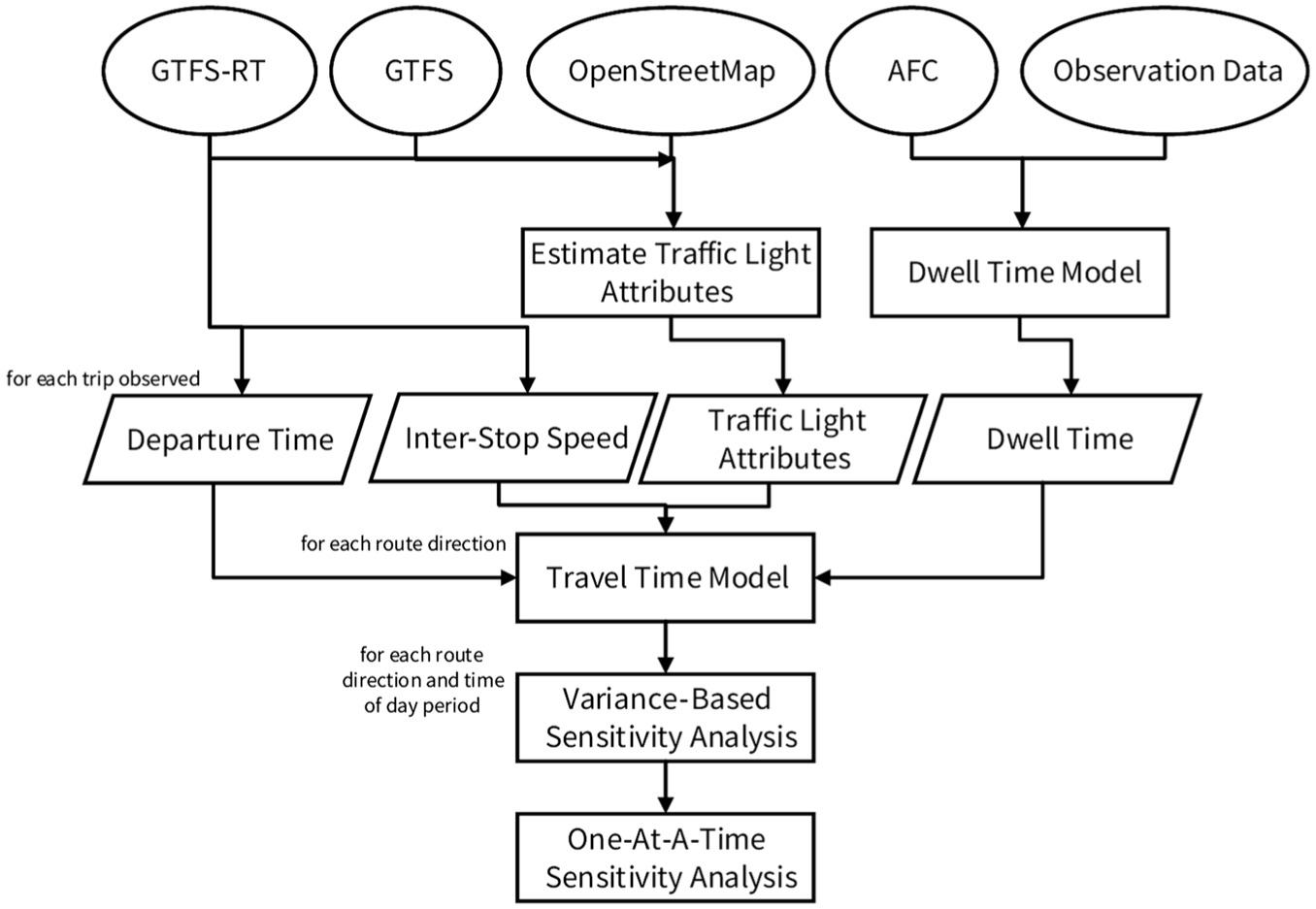
Research framework.
To get these detailed times, we use the General Transit Feed Specification (GTFS), GTFS Real Time (GTFS-RT), OpenStreetMap, Automated fare collection, and some ride-check observation data. The departure times and inter-stop times are directly obtained or calculated from the GTFS-RT feed. Given the lack of door-closing times, we estimate a simple dwell time model at the stop level using ride-check observation data and apply the model to the fare transaction data. The traffic light settings are also estimated following the methodology proposed by Fayazi et al. ( 8 ) as a result of data availability issues.
The decomposed travel times are then grouped by route direction and three different times of day and used for sensitivity analyses. Here, we focus on both the variance-based analysis ( 9 ), which is a global method that quantifies the proportion of variance that can be attributed to each variable. We also conduct a one-at-a-time sensitivity analysis to better illustrate the non-linearity between the input variables and the overall travel times. Since sensitivity analyses require varying one or more variables, we can adjust the inter-stop and dwell time variables given the observations. However, since signal timings are mostly fixed and not within the agency’s control, we calculate the resulting red-light waiting times given the arrival time at the signal and the signal timing plan as input.
We use the data provided by Société de Transport de Montréal on the island of Montréal in Canada as a case study. The system currently has 222 bus lines in operation, about 2,000 buses in the fleet, and more than 17,000 published bus trips on average weekdays. More detailed information with regard to the methodologies and data used in each step can be found below.
Defining the Trip Elements
The GTFS file provides detailed information on the planned services, such as schedules and geographical information for the routes and stops. Since it only publishes transit-related information based on stop arrival and departure times, we need to add more detailed information to better isolate each trip element for our analysis.
To split the routes into these elements, we used the route shape from GTFS and matched traffic light positions from OpenStreetMap, so that we can estimate the red-light waiting times in later steps using the vehicle location information. Since there may be additional traffic signals between two scheduled stops and inter-stop time variations will cause the red-light waiting times to change for these signals, we will split the stop-to-stop segment at these traffic lights so that we can attribute red-light waiting times to each signal along the route.
To reconstruct the travel and arrival times, we need to calculate four categories of information, the departure time from the first stop, a series of inter-stop times, a series of dwell times, and a series of red-light waiting times. Since most of our bus stops are on the near side, that is, right before the bus enters the intersection, The sequence of these times is typically ordered as follows: first, we depart from stop 1 at a given departure time, followed by the inter-stop time to stop 2, then the dwell time at stop 2 if applicable, and finally the red-light waiting time at stop 2 if applicable. Since red-light waiting times are the result of vehicle arrival time at the intersection and the timing plan, we will have to calculate them using the arrival time at the signal, based on vehicle position, and the estimated signal timing plan. The pattern then repeats itself for the following stop-to-stop pairs until the service destination. Thus, we define our input variables following the same logic for every trip. After the introduction of these times, we will provide an example to demonstrate the categorization in a separate section.
Estimating Traffic Signal Settings
Traffic signal timing plans change often since traffic levels vary constantly. In addition, because of roadworks, programming errors, or malfunctions, the planned signal timings are not necessarily what is operated. Unfortunately, as a result of data availability issues, we could not obtain the signal timings in real time. Thus, we will estimate the signal timings also using the aforementioned archived bus trajectory data.
Given the high density of signalized intersections, most of the traffic signals in Montréal use the coordinated timing plan to optimize traffic flow on major streets, as recommended by the National Cooperative Highway Research Program’s Signal Timing Manual ( 21 ). There are three principal parameters for a coordinated timing plan: cycle length, offset, and split. Cycle length is the time for a complete sequence of signal phases at an intersection ( 21 ). In Montréal, it is generally between 60 and 140 s, depending on the traffic volumes at the intersection. The offset is defined as the time offset between coordinated phases to a predefined synchronization point ( 21 ). They are used to offset the green or red phases to help vehicles progress through multiple intersections without stopping. The splits are the portion of green light plus clearance time allocated to each phase at an intersection ( 21 ). In this paper, we will focus on the green light time only, since the red times, and clearance times have the same effect on buses, that is, buses are not allowed to cross the intersection.
To estimate these three traffic signal settings, we mainly followed the methodology proposed by Fayazi et al. ( 8 ) with some minimal modifications to handle a few particularities of our local vehicle locations feed. The basic idea is to match stop times at a given traffic light observed over a given time of day by testing out various cycle lengths and signal offsets to see which combination fits the observations the best. Then, using a moving window, we can detect changes in traffic signal schedules, such as peak schedule versus off-peak schedule. Readers interested in the details can refer to the original paper cited above.
To verify the estimated signal settings, we conducted ride checks on board buses and point checks at intersections. The estimation errors are typically around 3 to 5 s. We consider this acceptable, as it is similar to the length of yellow lights and the errors observed in the original paper ( 8 ). As mentioned in the original paper, drivers have different risk tolerances toward yellow lights, some may treat it as a green light and some may treat it as a red light, thus causing some slight discrepancy in the estimated timing ( 8 ). For Montréal, we mainly use fixed signal timing plans with very little flexibility, which allows this estimation method to function well. Unfortunately, the sensitivity for more flexible timing plans and more aggressive transit signal priorities has to be left for future research.
Getting Departure Times and Inter-Stop Times
This step mainly uses the GTFS-RT data, which provides the actual bus arrival and departure times at stops, as well as detailed bus location and speed information around every 5 to 20 s. Using this information, we can directly obtain or calculate the departure times and inter-stop times needed for our analyses. Here, we used 3 months of archived data from January 8, 2024 to March 24, 2024.
Since this project focuses on travel times, outlier observations, such as major detours, might greatly affect the sensitivity of travel time, and agencies are typically aware of these types of travel time variations. Thus, we will remove these outliers from the analysis using Density-Based Spatial Clustering of Applications with Noise (DBSCAN) ( 22 ), which is a density-based algorithm to identify clusters and outliers in the data. To reiterate, because of various statistical distributions observed in previous research ( 14 ), we don’t want to make any assumptions about the data distribution. In addition, given the mixture travel time distribution observed (e.g., Figure 1), there may be many small clusters of travel times that might be more extreme but meaningful. We, therefore, choose this method for cluster detections and outlier removals. For each trip, we compare the similarities of the trip departure, travel time, and delay observation for all trips. The outliers that are not similar to other observations, such as significant delays and unusually long or short travel times, are identified and removed from the analysis.
Estimating Dwell Times
The dwell time is defined as the time for passengers boarding and alighting the bus ( 10 ). However, because of the lack of door-closing times and some drivers leaving the door open for ventilation while waiting for the red lights, we will estimate a dwell time model using ride-check observation data.
The ride-check observations include detailed door opening times, number of boardings, number of alightings, and any kneeling or ramp usages. The end of dwell time is defined as either the door-closing times collected on board, or 5 s after the last passenger boarding or alighting in case the driver leaves the door open. Then, using roughly 25,000 dwell time observations over two years, we estimated a simple dwell time model using linear regression using these observations, following the example from Dueker et al. ( 6 ). For trips without on-board observations, we used the origin–destination from fare transaction data to obtain the passenger counts at each stop, and applied the estimated dwell time model for decomposition.
We acknowledge that the dwell time model is in no way perfect, as there remain some issues with the agency’s ridership matching algorithm, our ridership observations can still be improved, and dwell time variations deserve more research on their own. As the agency improves the origin and destination matching algorithm, future researchers could add more variables with regard to the overall passenger flow, ridership variations given bus bunching, trip purposes, and so on. However, because of the time limit, we will settle with these imperfections for the moment and only focus on the sensitivity analyses at a given stop. We will leave improving dwell time models, passenger flow models, understanding ridership variations, and passenger arrival patterns as a future research task.
Example of Decomposing a Stop-to-Stop Travel Time Observation
Finally, to sum up these detailed time breakdowns, Figure 3 shows an example time-distance diagram for one stop-to-stop travel time observation. Here, we have a stop-to-stop travel time observation where the bus starts from the terminal (distance 0 m) and travels to stop 2 on the route (140 m after the terminal). From the time-distance graph, we can see that the stop-to-stop travel time is 2 min and 50 s from 7:22:51 to 7:25:41. The stop-to-stop travel time is split first into the inter-stop time which is the time it took to travel to the next stop from 7:22:51 to 7:24:41. For our example, despite the bus being 20 m away from the stop for over a minute, the door did not open because of congestion, so the inter-stop travel time is around 1 min and 50 s. Then, as the bus stops at the second stop, the stopped times are split into dwell times according to the dwell time model, which is estimated to be around 20 s, given the estimated passenger boarding and alighting numbers. Then, the bus stays at the near-side stop for the remainder of the red light doing nothing, until the green light activates at 7:25:41 according to the estimated timing plan. Thus, the estimated red-light waiting time is around 40 s. The decomposition is repeated and performed for every stop-to-stop observation that follows until the end of the route and for every recorded trip on a given route direction.
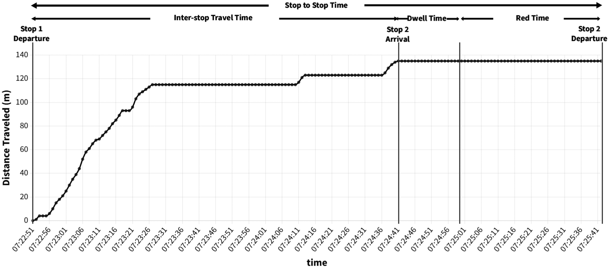
Example: Splitting a stop-to-stop travel time observation.
Sensitivity Analyses
Sensitivity analyses are typically used to attribute the variation of model outputs to the input space. In this paper, we analyze the sensitivities by route directions and by three time-of-day periods, since the signal synchronization, ridership pattern, and traffic conditions may be different. There are typically two main categories of sensitivity analyses: one-at-a-time and global analyses ( 9 ). We will provide a quick introduction to both methods in this section.
Variance-Based Sensitivity Analysis
Given the complexity and non-linearity typically observed in previous travel-time studies, we first consider the variance-based sensitivity analysis (also referred to as the Sobol method). Variance-based sensitivity analysis is a commonly used method that can handle non-linearities between input and output results. It is typically used in analyzing large environmental or biological models ( 9 ), albeit rarely used in transportation fields. It is also included in many statistical or optimization software packages.
A quick summary of the method is that it varies all input variables at the same time. It then sends the inputs to the model, for example, a travel time model, which is considered a black box. Next, it decomposes the total variance of the model output into partial variances, that is, the percentage of total variance, and attributes the partial variances to individual input variables. Readers who are interested in more detailed derivations and explanations can refer to Saltelli et al. ( 9 ).
To generate the samples needed to calculate these indices, researchers typically conduct a Monte Carlo simulation ( 9 ) to uniformly sample all input space. However, given the various travel time distributions observed from previous studies ( 14 ), we decided to use the observed trips as inputs to avoid making assumptions about the data distribution.
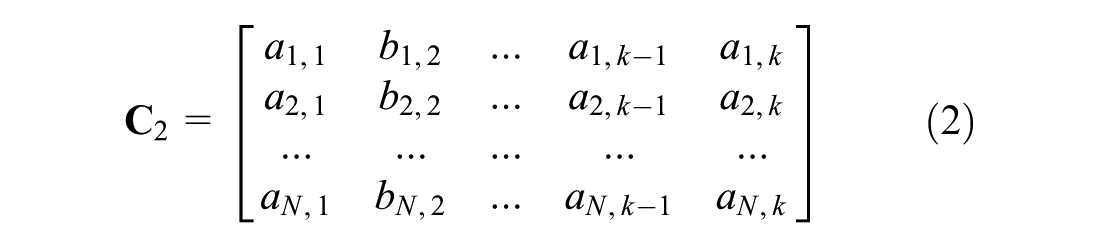
The method would then randomly split our trip observations into two matrices

Sensitivity analysis attributes the output variance to the variation in some input variables while holding other variables constant. For the variance-based analysis,
In simpler terms, the method uses one observed trip as a base case, then replaces different elements of the trip with the observations from another trip, that is, what would have happened if the bus were to spend a different amount of time at a given section. If the analysis includes a change to make an extra stop, the inter-stop times cannot be directly applied because of the extra slowdown and acceleration time needed. In this case, we will estimate and include the time changes caused by additional or skipped stops. Similarly, new red-light waiting times are recalculated using the updated arrival time or signal timing plan.
Finally, the sensitivity indices are estimated using original travel times observed for trips in
The model produces two main indices, the first-order index and the total-order index. The first-order index is calculated as the percentage of total variance reduced if one variable were fixed ( 9 ). In other words, the first-order index is the percentage of the total variance caused by the variation of a given input variable, without interaction effects. It is formulated as

Similarly, the total-order index is calculated as the complement of the variance produced by varying all but one variable, normalized by the total variance ( 9 ). In other words, it shows the percentage of the total variance caused by the variation of a given input variable, with interaction effects. It is formulated as

These indices lie between 0 and 1, since they represent a percentage of total variance. These indices can also be used for ranking purposes according to the share of total variance attributed to each input. The first-order indices typically add up to less than 1 because of the exclusion of interaction effects. Similarly, the sum of total-order indices will typically exceed 1 because of counting interaction effects multiple times.
Although it is theoretically possible to calculate any n-th order sensitivity indices, they are not practical to calculate or apply. Assuming there are
One-At-A-Time Sensitivity Analysis
One-at-a-time sensitivity analysis is a typical direct approach to see the effect of changing one input on the output ( 23 ). The steps are incrementing one input variable while keeping the others constant, then returning the changed input to its original value, and repeatedly changing the other variables in the same way. Sensitivities are typically measured by the partial derivatives, that is, the amount of change observed in the output by changing the input by 1.
Given its simplicity, the method does not examine the entire input space like the variance-based method described above, and thus the results do not show the interaction effects and non-linearity ( 23 ) between variables. Given its easy-to-understand nature, we decided to include this method to better illustrate the sensitivity results and non-linearity between trip travel times and various trip elements. However, we will not aggregate the results into one number in this paper because of the limitations mentioned above.
Case Study: Montréal
In this section, we present the sensitivity results using the data from Montréal. First, we will provide a quick overview of the variance-based global analysis results for 20 selected routes operating in the central part of Montréal, so that readers can have an understanding of the most important factor affecting each travel time component. We will then use the westbound Route 27, the northbound Route 30, and the eastbound Route 97 as examples to demonstrate more route-specific analyses. The data and conclusions may be specific to Montréal and the routes analyzed, but the readers can nevertheless adapt the methodology for their cities and draw their own conclusions given their specific local contexts.
Overall Variance-Based Sensitivity Results for 20 Selected Routes
Here, we summarize the most important factors affecting 20 selected routes in the central areas of Montréal. These routes typically travel through areas with a higher population density, mixed-use developments, and higher traffic light density. First, we will show the most important factors for each travel time component, that is, inter-stop travel times, dwell times, and red-light waiting times. Then, we will present the sensitivity results for the overall trip travel times.
Most Important Factors Affecting Inter-Stop Travel Times and Dwell Times
The differences between first-order and total-order sensitivities are very small for the overall inter-stop and dwell times. Therefore, the results suggest little interaction effects contributing to the variation of inter-stop times and dwell times.
The important factors affecting the overall inter-stop times are all inter-stop variables. As we categorized the trips by time-of-day periods, the inter-stop travel times are relatively similar. Therefore, they are not as sensitive to the departure time changes as the overall trip times and red-light waiting times as we will demonstrate later. The overall inter-stop time is also not very sensitive to the signal timing plan changes, since the vehicles would still need to travel to the next stop in similar traffic conditions.
Similarly, the most important factors affecting the overall dwell times are all ridership variables for the stops. This makes sense since dwell times only include the times for passenger activities as defined by Transit Capacity and Quality of Service Manual ( 10 ) (e.g., Figure 3), and we do not yet consider the ridership variations caused by vehicle interactions or schedule adherence issues in this paper. We, therefore, emphasize the future research need to better understand ridership variations caused by vehicle interactions, as well as incorporating passenger arrival patterns into the variance decomposition models.
Most Important Factors Affecting Red-Light Waiting Times
Figure 4 shows the most important factors contributing to the overall red-light waiting time variations. Again, according to the Transit Capacity and Quality of Service Manual ( 10 ), red-light waiting times are the times stopped after passenger boardings and alightings are complete (e.g., Figure 3).
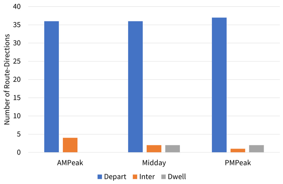
Most important factors contributing to overall red light waiting time variations for 20 routes at various time-of-day periods.
The most important factor for the red-light waiting times on the 20 routes (40 route directions) analyzed is almost all departure time changes at the first stop. The number of route directions with the departure times as the most important factor remains stable throughout the day, roughly 36 to 37. The number of route directions with other factors as the most important is generally around 3 to 4. As the day goes on, the number of route directions with inter-stop times as the most important factor slightly decreases, but the number of route directions with dwell times as the most important factor increases slightly as the ridership variation becomes higher later in the day. Still, it is very important to consider the departure time when analyzing red-light waiting time variations.
The 20 routes analyzed in this paper are all located near the center of the city and thus have a higher density of traffic lights. The red-light waiting time counts toward 20% to 25% of trip travel times for these 20 routes, and it is the category with relatively high variance. This observation shows that it is really important for planners to choose the right departure time. If the planners want to reduce the red-light waiting time variations, there is a need to consider how departure time changes affect red-light waiting time variations when adjusting the schedules.
Currently, the signals follow a fixed timing plan with varying cycle lengths depending on the importance of an intersection. Larger intersections have longer cycle lengths (e.g., 140 s), and quieter intersections have shorter cycle lengths (e.g., 60 s). Thus, green waves do not necessarily line up perfectly for the entire bus route at all times. The importance of departure time arises from how synchronized or desynchronized the signals are. To reiterate, since the travel times can be defined as the departure time from the first stop, plus a series of dwell times, inter-stop times, and red-light waiting times, the red-light waiting times down the route depend on the departure time at the first stop, and the previous inter-stop, dwell, and red-light waiting times. Thus, the departure time at the first stop roughly sets the synchronization pattern further down the route.
Readers can consider a simple example. Buses leave intersection 1 at perfect 5-min intervals at an intersection with cycle lengths of 100 s that is, every 3 cycles. For example, departure times can be at 0, 5, 10 min, and so forth, past the hour. Buses then travel to intersection 2 with the same 1-min travel time, thus arriving at the intersection at 1, 6, and 11 min past the hour. If the signal cycles at intersection 2 is 120 s and the green light starts at 0, 2, 4, 6, 8, 10, and 12 min past the hour with 53 s green time and 7 s for yellow and clearance times, the first and the third bus will have to wait for red lights at intersection 2 while the second does not. Therefore, every other bus will have to spend longer times trying to pass intersection 2.
Given the importance of departure time on red-light waiting times, planners could add adequate schedule padding to ensure the buses have similar travel times or to optimize for specific departure times to include the red-light waiting time variations in planned travel times. Another potential strategy to reduce the red-light waiting time variations could be a more aggressive signal priority that is applied more in advance to reduce the significance of departure times. Moreover, not all trips are able to depart exactly on time, potentially as a result of residual delays from earlier trips, waiting for a late passenger, or some other similar reason. Thus, it is also important for future researchers to find a way to better provide signal priority to buses while considering the varying cycle lengths and potential departure, inter-stop, and dwell time variations.
In addition, a common assumption used when creating schedules and optimizing vehicle assignments is to assume travel times remain the same within a few minutes. Intuitively, traffic congestion levels may stay similar and ridership may remain similar if we change the departure time by a few minutes. However, as shown here, the red-light waiting times are significantly affected by departure time changes. Thus, planners need to be careful when optimizing bus schedules since the constant travel time assumption may not be applicable everywhere.
Most Important Factors Affecting Overall Trip Travel Times
Figure 5 shows the most important factors contributing to overall trip time variations for 20 routes at various time-of-day periods. As we can observe from the figure, the most important factor can change throughout the day. Thus, planners may need to consider different strategies to improve transit reliability at various time-of-day periods.
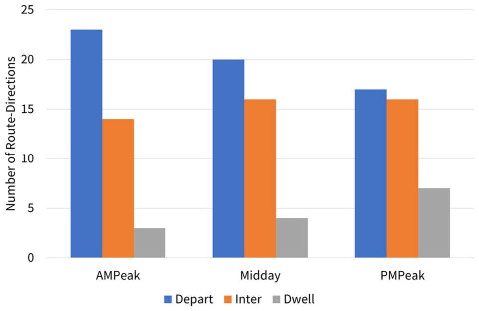
Most important factors contributing to overall trip time variations for 20 routes at various time-of-day periods.
The departure time contributes the most to the trip travel time variations for most of the routes analyzed. As shown in earlier subsections, departure times are very important for red-light waiting times, but not as important for dwell and inter-stop times. Since red-light waiting times are also a big part of the overall travel times, the results suggest that variations in red-light waiting times contribute greatly to the overall travel time variation. Moreover, there are more possibilities for buses to get delayed or run early while interacting with traffic signals or congestion compared with the last stop on the route.
However, the number of route directions with departure time as the most important factor decreases as the day goes on, decreasing from 23 route directions during the morning peak to 20 route directions during midday to 17 route directions during the evening peak. The number of routes having inter-stops as their most important factor grows from 14 to 16 from morning peak to midday. The number of route directions with dwell time as their most important factor grows from 3 to 7 throughout the day. As we will demonstrate in the later sections, inter-stop time and dwell-time variations become higher later in the day.
We believe this could be correlated to the travel pattern changes or signal timing plan changes. For the morning peak, the traffic patterns and ridership patterns are relatively stable, since most people are going to work or school, as shops and other destinations are not yet open. As the day goes on, more shops and restaurants begin to open, traffic congestion and ridership can fluctuate and become more significant on some routes or certain sections. Thus, planners may consider other ways to improve reliability, such as implementing bus lanes.
In addition, the changes may correlate with the three signal timing plan changes during the day as well. During the off-peak hours, such as midday, midnight, and weekends, the signals typically use the same timing plan. During the two peaks, the timing plan is changed to facilitate travel toward downtown in the morning or away from downtown in the evening. Planners, therefore, need also to consider how travel directions might potentially affect the overall travel times.
Detailed Variance-Based Sensitivity Results for Three Example Routes
In this section, we will use the results from three different routes analyzed to illustrate the different issues and factors affecting transit travel time reliability. These three chosen examples are based on the most important issues discussed in the earlier section and are somewhat representative of other routes in our study. However, planners want to be mindful of different local contexts and configurations for different routes, although the analysis process is similar. First, we will use the westbound Route 27 as an example to illustrate the impact of departure time variations, which interact with signal timing plans and in turn affect the red-light waiting times. We will then discuss the northbound Route 30, which faces congestion variations in a popular shopping area. Finally, we will examine the eastbound Route 97, which has high ridership variations at the stop in front of the metro station.
Westbound Route 27: Departure Time
Route 27 is relatively short and straightforward. The 4.1-km route operates on a secondary corridor Saint-Joseph Boulevard through a densely populated neighborhood on the eastern side of the city. Its daily ridership is an average of 2,400 passengers, mainly feeding passengers into the metro service which is its western terminus. Its peak direction headway is 9 to 12 min with roughly 40 to 50 passengers on board. For off-peak directions or hours, the headway is typically between 23 and 27 min with roughly 25 to 35 passengers on board. The planned one-way travel times are between 19 and 24 min. During peak hours, there is also a limited stop service that supplements this local service in the peak direction only with similar headways and ridership numbers. Another factor that makes this route interesting is that it has the highest traffic signal density within the network. On average, there is a signal every 170 m, with the distance between signals being as little as 50 to 75 m on some sections.
Since we decomposed each stop-to-stop segment into four variables, departure time at the first stop, inter-stop times, dwell times, and signal timing plans, the 22-stop service has 83 input variables. As mentioned in the methodology section, we cannot calculate detailed results showing every possible combination of variables and their interactions. To demonstrate the computational complexity, the number of 41st-order sensitivity indices for this route direction would be

Example: Sensitivity indices for westbound Route 27.
The sensitivity results for the overall inter-stop and dwell times are similar to the observations in previous sections. From the figure, we can observe that the sensitivity indices are higher near the northeastern side of the route, at almost 0.7, meaning that with interaction effects, 70% of the total travel time variance can be attributed to the variables and their interactions in this area. Given the small overall travel time variations, at around 2 to 3 min, this area alone could be attributed 1.4 to 2.1 min of variation. The most important factor is the departure times, the first-order sensitivities are around 8%, and the total-order indices remain around 60% to 70%. This result again suggests that departure time alone does not contribute much toward the overall red-light waiting time variation. However, the interaction effects of departure time contribute significantly toward the overall travel time variation. Similar to previous sections, the most important factor affecting the overall dwell time variation is the stop with the largest ridership variance, located in the lower part of the map for the morning peak, and the middle of the map for the midday and evening peak, contributing around 50% of the total variance with interaction effects.
For the overall travel time variations, the most important factor for both the first-order and total-order indices is the departure times at the first stop for all three time-of-day periods, shown as a dark red circle on top of the figures. Table 1 shows the departure time sensitivity results with their equivalence in seconds calculated using the standard deviation. From the table, we can see that 8% of the total variance during the morning peak can be attributed to the departure time without interaction effects (first-order). For context, the standard deviation is roughly 10 s. If we include the interaction effects (total-order index), the departure time attributes 67% of the total variance during the morning peak (roughly 83 s standard deviation). However, the sensitivity for departure time changes slightly later in the day. The first-order indices for the midday and evening peak periods are 6% and 8%. The total-order indices for the midday and evening peak periods are 47% and 42%.
Departure Time Sensitivity Results for Westbound Route 27
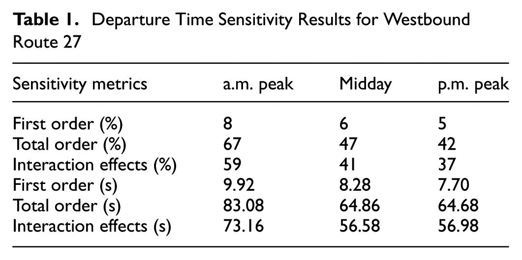
Since the overall travel time includes the sum of all red-light waiting times, where the importance of departure time dominates, and all inter-stop and dwell times, where departure time is not as significant. This result highlights the importance of red-light waiting time variation on the overall travel time variance.
More specifically, the signal cycle lengths along this route are 80, 90, 100, and 120 s, with a least common multiple of 3,600 s. Thus, for any given departure time within 1 h, the green wave patterns and the red-light waiting times will be different. We therefore emphasize the need for transit planners to pay more attention to the base timing of traffic signals and their interactions with transit vehicles when analyzing or planning for travel times.
The second most important factor for the overall trip travel times is the traffic light timing changes, shown in the sections and points near the top of the maps. During the study period, there was a traffic light timing plan change as a result of a newly implemented bike lane as well as improved pedestrian crossings. The change in signal timing contributed on average 2% of the total variance without interaction effects (around 2 s standard deviation), but 20% of the total variance with interaction effects (24 to 30 s standard deviation) for all three time-of-day periods. Thus, a change in traffic light timing may not cause a significant variation in travel times locally, but planners must consider the potential chain reaction it has with downstream sections of the route when evaluating the impacts of signal timing plan changes.
To summarize, the above observations show strong interaction effects between input variables for the overall trip time and the overall red-light waiting times, given the larger differences between first-order and total-order sensitivity indices. Thus, the result emphasizes the need for planners to choose the departure times at the first stop carefully and better understand the interaction effects in transit travel times for planning. The results also show little interaction effects for the inter-stop times and dwell times given our assumptions, which makes it easier for planners to improve reliability for times in these two categories.
We will try to demonstrate the potential variations caused by different variables and the non-linear relationship by applying the one-at-a-time analysis on this route as an example in the next section.
Northbound Route 30: Inter-stop Time
Route 30 is a 11.3-km route, running north–south on corridors Saint-Denis and Saint-Hubert. The population density around these two corridors is high. Given the mixed-use zoning commonly found in the central areas of Montréal, these two streets are also busy shopping areas. Therefore, this route passes destinations that are popular for locals and tourists. However, since this route duplicates part of the Orange Line metro service and passengers generally prefer the faster congestion-free metro, the ridership on this route is not high (around 2,000 to 2,500 during average weekdays) and the service frequency is quite low at around 30 to 35 min. As for travel times, the planned times are between 44 to 64 min depending on time of the day, and the standard deviation of the overall travel times is around 4 min in the morning peak, 5.5 min around noon, and 8 min at the afternoon peak.
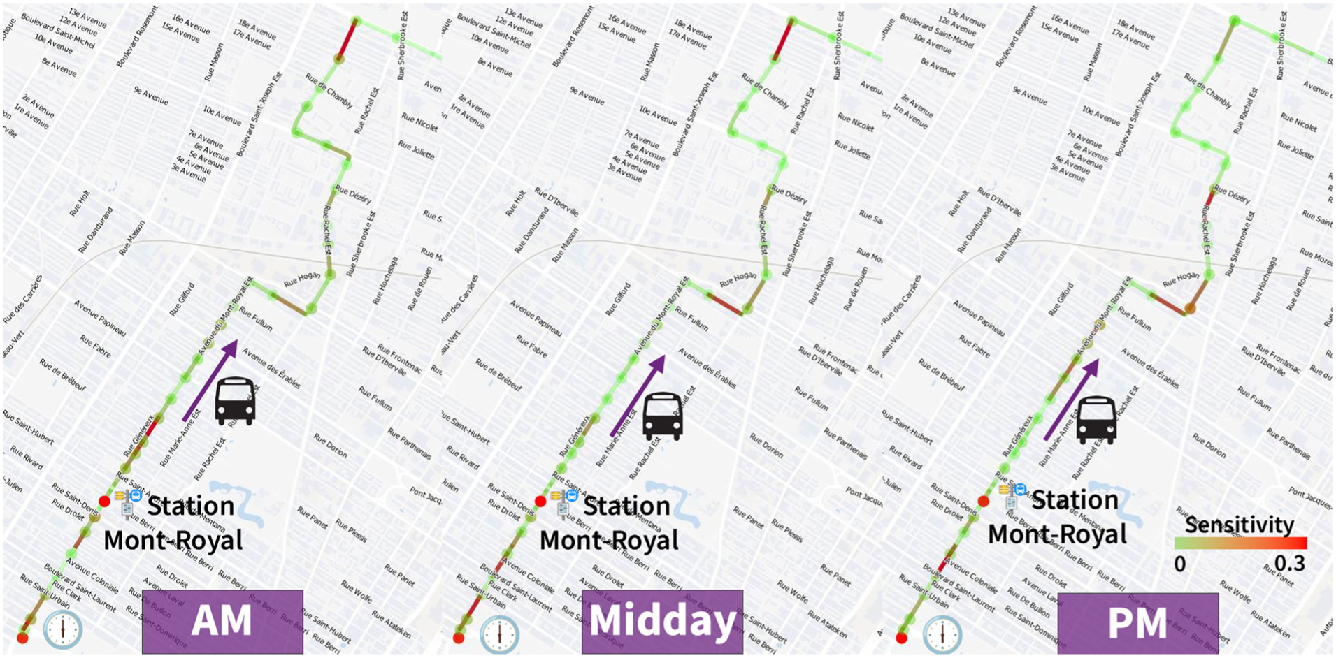
Figure 7 shows the general alignment of the route and the sensitivity indices on the map, with the two main problem areas, Plaza Saint-Hubert and Saint-Denis, marked on the map in the central and south side. The departure times (marked as the right-most dot in the figure) are the most important during the morning peak, contributing around 20% of the variation with interaction effects. However, the importance remains relatively stable during the day. The inter-stop times at Plaza Saint-Hubert start to contribute more variance to the overall travel times. The sensitivity results for the inter-stop times at Plaza Saint-Hubert gradually rise during the day; around 30% of the variation could be attributed here during midday and the afternoon peaks.
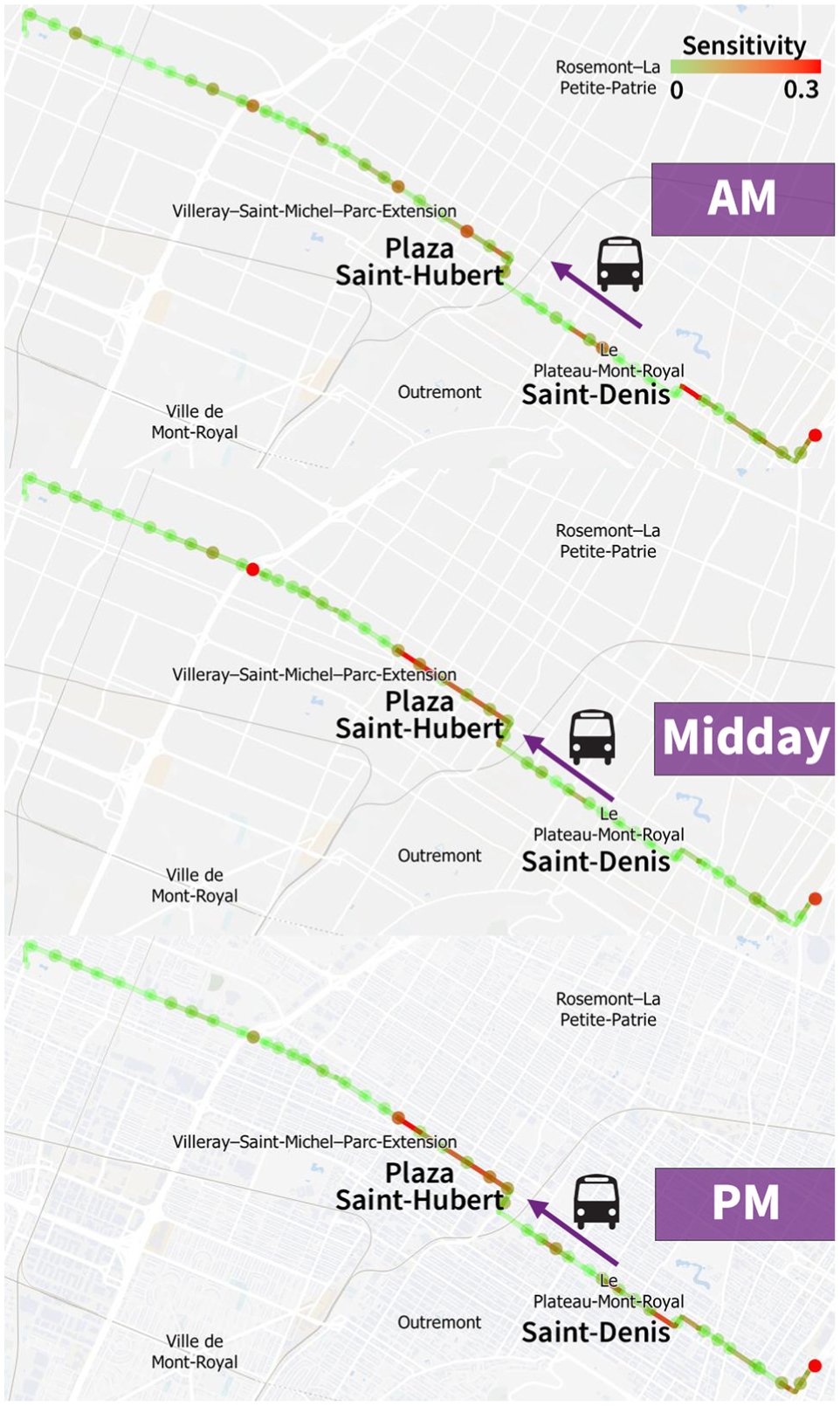
Example: Sensitivity indices for northbound Route 30.
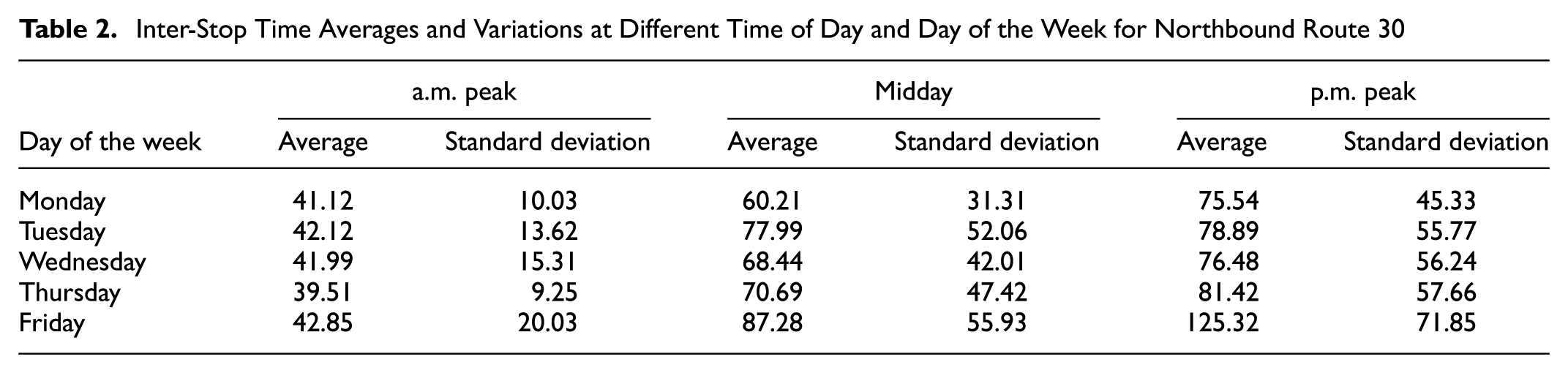
The main issues identified for this route are the inter-stop times, unsurprisingly given traffic congestion, since not everyone uses transit to access these two popular areas, despite having good transit connections. In this section, we will use the Plaza Saint-Hubert area as an example, since it is the top issue for the midday and the afternoon peak, although the variation is a lot smaller in the morning peak (total-order index less than 1%). Table 2 shows some simple statistics to highlight the day-to-day variations as well as the within-day variations of inter-stop time. From the table, we can observe that the average inter-stop time grows higher as the day progresses, where the morning peak has the lowest averages and standard deviation regardless of day of the week, and the afternoon peak has the highest averages and variation regardless of day of the week. This matches our expectation, since the shops and restaurants in this popular area are not yet open during the morning peak. Therefore, the area attracts fewer visitors and traffic at this time. Around noon, shops and restaurants start to open their doors and remain open until late at night, attracting more visitors during the later time of the day, thus increasing the traffic and travel time. There are also obvious within-week variations for the travel times. From the table, we can see that Friday has the highest travel time averages and variations. We hypothesize that some people are able to work from home on Fridays, therefore having more freedom in their preferred times to visit the area. Similarly, Monday generally has lower averages and standard deviations, which also makes sense since some shops close on Mondays, so there are slightly fewer trip attractions in the area. However, since the agency uses the same schedule for Monday and Friday, and Friday has significantly higher figures than Monday (three times the average and standard deviations), planners should be ready to deal with such variations when scheduling travel time and recovery times.
Inter-Stop Time Averages and Variations at Different Time of Day and Day of the Week for Northbound Route 30
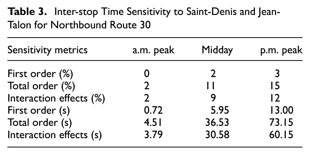
Given the significant inter-stop travel time changes mentioned above, we want to discuss the overall travel time variations that can be attributed to this short route segment. Table 3 shows the sensitivity analyses results for the inter-stop times to the intersection at Saint-Hubert and Jean-Talon (near the top end of the Plaza Saint-Hubert area in Figure 7). Again, we can see that the morning peak has the lowest sensitivity results because of the consistent short travel times, at around 2% of the total travel time variation and around 4.5 s in time. Then, as the day goes on, the sensitivity for this specific route segment grows as the traffic becomes worse and more varied, and the sensitivity of this segment increases as the total-order index reaches 15% and 73 s in time. The total-order index increases especially fast as expected, since the traffic variations in this popular shopping area are low in the morning peak, buses can generally clear the segment without much queuing. In the afternoon, on the other hand, traffic is worse, and buses may need to wait for an extra cycle or two to clear this segment. Therefore, buses may face a slightly different green wave pattern for the upcoming intersections as the traffic signals are not all synchronized nor have the same cycle lengths. As a result, the departure times matter slightly less for this route in the midday and afternoon peak periods, as the congestion levels may also affect the upcoming signal patterns.
Inter-stop Time Sensitivity to Saint-Denis and Jean-Talon for Northbound Route 30
Eastbound Route 97: Dwell Time
Route 97 is a 6.7-km route, part of the “frequent” service network, that runs along Avenue du Mont-Royal in Montréal. Avenue du Mont-Royal is an important corridor for the city of Montréal. The population density is relatively high. The western end connects to the Mont-Royal park, allowing easy access for outdoor leisure activities for local residents and tourists. With mixed-use zoning, it is also an important destination for shopping, cultural, and dining opportunities. It is, therefore, a popular destination for locals and tourists. With a connection to the metro station at Station Mont-Royal, the route also allows riders from other parts of the city to visit the area. Its daily ridership is around 6,000 passengers, and the ridership generally increases during peak shopping season, reaching as high as 9,000 passengers. The headway for the afternoon peak is 7 to 10 min, the planned one-way travel times are between 30 and 44 min, and some trips consistently have roughly 30 passengers waiting to board here.
Figure 8 shows the sensitivity indices on the map, with varied sensitivity results. However, the top two factors in the variance attributed are the departure time (the dot on the bottom left) and the dwell time at Station Mont-Royal. The percentage of variance attributed to these two variables remains relatively stable during the day. For the departure time, it is generally between 15% and 20%. For the dwell time at Station Mont-Royal, it is slightly higher at between 17% and 20%. There are also a few sections with higher inter-stop sensitivity. However, the sensitivities are generally related to the congestion and remain less than the dwell time at Station Mont-Royal. Therefore, this section will mainly focus on the dwell time at Station Mont-Royal area as an example.
Example: Sensitivity indices for eastbound Route 97.
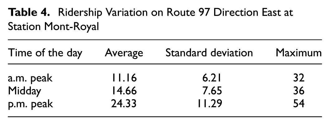
Here, we use the stop in front of the metro station as an example to illustrate the variations. Table 4 shows some simple statistics to highlight the ridership variations for this route. From the table, we can observe that the average ridership grows higher as the day progresses. This matches our expectation, since the shops and restaurants are not yet open during the morning peak, and the routes are used mainly by regular commuters going to work. Around noon, shops and restaurants start to open their doors until late at night, attracting more visitors later in the day. The variation of ridership also grows higher, especially during the afternoon peak. The reason could be that people may choose to enjoy leisure activities after work, so that the ridership variation comes from not only the variations of commuters going home but also variations in leisure trips. Again, other cities may have different travel patterns and ridership variations compared with Montréal. Therefore, the results shown here are only used to illustrate the method, and other researchers could adopt similar analyses for their specific contexts.
Ridership Variation on Route 97 Direction East at Station Mont-Royal
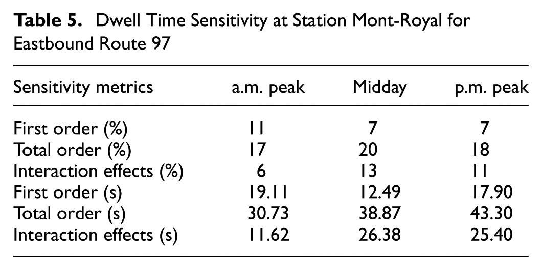
As mentioned above, the most important variable associated with this route, this direction more specifically, is the dwell-time variation for the stop directly in front of the metro station. Table 5 shows the sensitivity analysis results for the dwell time at Station Mont-Royal, given the standard deviation of the overall travel time is generally around 3 min for the morning peak and midday, then 4 min during the evening peak, we also estimated the variance contribution in seconds. From the table, we can see that the total variance attributed to the dwell time at this stop remains relatively stable, around 7% to 11% for first-order and around 17% to 20% for total-order effects, despite the increase in average ridership and ridership variation later in the day. However, as we convert the percentage of variance attributed to times, we can observe the relatively stable first-order effects but an increase in total-order effects. Similar to the inter-stop times mentioned above, as the ridership increases, especially for the bus with 54 people waiting to board, the longer dwell time may cause the bus to miss one or two traffic light cycles and have to depart at the following traffic light cycle, which would cause a slight deviation in green wave patterns. Therefore, the departure time is a close second in the importance of the sensitivity indices, despite more traffic lights being synchronized in longer sections compared with route 27.
Dwell Time Sensitivity at Station Mont-Royal for Eastbound Route 97
As a limitation, the algorithm to infer boarding and alighting locations for each passenger is still relatively new for the agencies in the region, so the estimations here are not very precise for more detailed analyses on passenger flows. As the agencies improve the algorithm to estimate boarding and alighting locations, future researchers could do more analysis into the associated ridership variations, such as inferring trip purpose, passenger arrival patterns, ridership variation given vehicle bunching, and so on. Future studies could then improve on this study to be more precise on dwell time variations, which could potentially help agencies better plan for these ridership and dwell time variations.
Discussion
The three case studies, Routes 27, 30, and 97, show three different sources of travel time variation. They are somewhat representative of the 20 routes chosen, traveling around the center of the city with high population density and mixed land use. The variability could be linked to the various specific operational and geographic contexts of the route, for example, signal synchronization, ridership, trip purpose, congestion, and land use. The sensitivity analyses across these routes demonstrate the varying influence of departure time, inter-stop time, and dwell time, and emphasize the importance of understanding interaction effects in transit planning. Planners should also be prepared to plan the temporal variations observed, since the trip elements may have different importance during the day.
In all three cases, the total-order sensitivity indices were significantly higher than first-order indices, emphasizing that many transit delays are not caused by single variables alone but by their interactions. For example, departure times determine roughly how the signal timings are likely to be for the trip. Gaining or missing a traffic signal cycle as a result of traffic or ridership variation would be relative to the green wave pattern determined at the departure time. Therefore, these interaction effects highlight the need to tailor transit priority strategies according to the operational and geographical contexts of the route, although the analysis method could be generalized combined with the local contexts and planners’ local knowledge.
One-at-a-Time Sensitivity Results for Westbound Route 27
In this section, we will attempt to demonstrate the non-linear relationship between each trip step and the trip travel time. As mentioned before, because of the limitation of one-at-a-time analysis, we will not aggregate the results into one number. As in the previous section, we will again use a westbound Route 27 trip during the morning peak as an example. Similar analyses can be carried out for the other routes.
Changing Dwell Time or Inter-Stop Time
Similar to previous sections, we can also examine the potential impact of ridership variation or inter-stop time variation on trip travel times while keeping the same departure time and traffic signal settings from the same median observation.
As shown in the previous section, the importance of dwell time and inter-stop times is high for a stop at the western half of Route 27. Figure 9 shows the relationship between a time increase in either dwell or inter-stop times and the resulting red-light waiting time and trip travel times.
Given the median observation, the bus completes the stop at 6:41:20 while the traffic light is green, and the traffic light would switch to red at 6:41:30. Therefore, the bus has 10 s to clear the intersection. If for some reason, the bus spends extra time traveling to the stop or picking up passengers, there are different impacts on the red-light waiting times and the travel times.
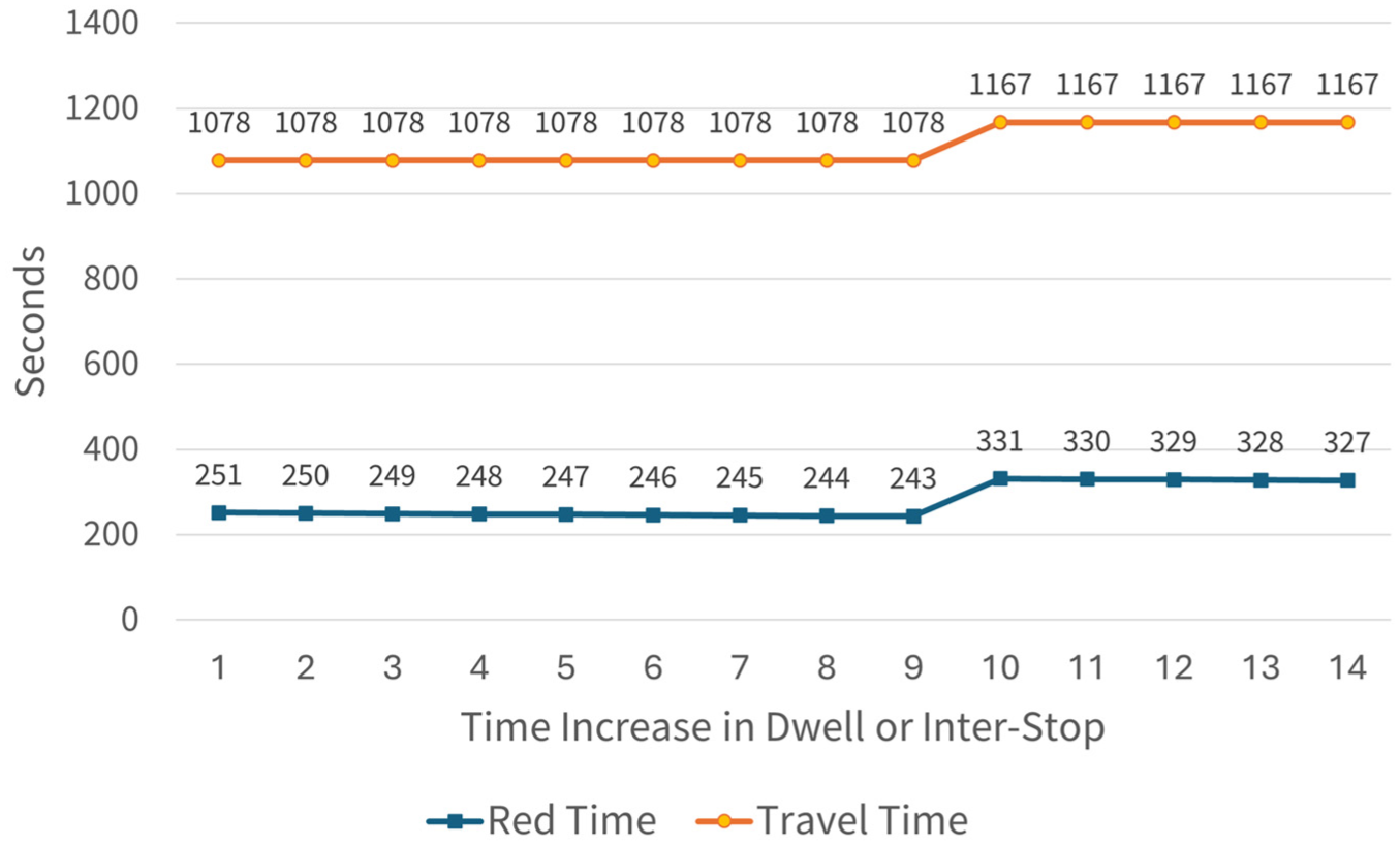
One-at-a-time analysis for dwell time or inter-stop time changes.
For red-light waiting times, if we add less than 10 s, the overall red-light waiting times decrease. This makes sense because we will wait less at the next red light given the longer time spent on this specific section. For the next traffic signal, the arrival time of the median observation is at around 6:42:00, given the green light comes on at 6:42:18, the red-light waiting time is around 18 s. If we can pass the current intersection with a small delay, say 1 s, the bus would then arrive at 6:42:01, which means 1 s less for the red-light waiting time at the next intersection. The overall travel time stays the same if we add less than 10 s. This makes sense, since we would depart the next intersection at the same green light. Thus, the red light at the next intersection absorbed the extra time needed at this given stop, and there would be no impact on downstream travel times.
If we add 10 s, the bus would arrive at 6:41:30, exactly when the red light comes on at this intersection. We would not be able to pass the intersection, and the bus would then depart when the next green light starts at 6:42:33, adding 63 s to the total red-light waiting time. We would then update the potential arrival times for the next stop, which would be 6:43:13. Checking the signal timing plan, the next green phase activates at 6:43:58, resulting in 45 s of red-light waiting time. The bus would then depart the next intersection at 6:54:58. Then, given the 20-s cycle length difference to the third intersection, the bus would pass during the green phase, rather than the red phase in the median observation, reducing 20 s of additional red-light waiting time. The calculation would repeat itself at every stop and intersection until the bus reaches the terminal. Unfortunately, the bus would not be able to catch up for these additional times, which would give a total of around 88 extra seconds waiting for red lights or extra travel times, similar to a traffic light cycle.
To summarize, the differences between the overall red-light waiting time and the overall travel time are similar but not the same. Red time would potentially absorb additional “useful” time spent traveling to the stop or picking up the passenger. Unless the bus misses a green phase, which would then cause an increase in the red time waiting times, then start decreasing again to absorb additional times needed. However, for the overall travel times, it stays relatively stable since it can be considered as the sum of inter-stop, dwell, and red-light waiting times. As red-light waiting times could potentially absorb some of the extra inter-stop or dwell times, the sums would not change, unless the bus missed a green light and departs one signal cycle late. Planners can potentially look at the risks of not going through an intersection when evaluating the sensitive elements on a given route.
However, a limitation of our study is that the vehicle delays also cause ridership variations. If the vehicle is delayed, it may pick up additional passengers who are supposed to catch the next trip. Similarly, delays on the previous trips might affect the ridership on this trip. Therefore, we need further research into the interaction effects between ridership and delays, the interaction between transit vehicles, as well as the potential passenger arrival patterns at stops to improve our model and analyses.
Changing Traffic Light Settings
As seen from previous sections, the traffic signal timing changes were the second most important factor for this route. During the analysis period, there was one single change in the traffic light timing plan for a newly implemented cycle path, as well as an improved pedestrian crossing. Three consecutive signals were affected by this change (the 3rd, 4th, and 5th signals, shown as red horizontal lines, from the start of the route in Figure 10). In the new timing plan, there is a dedicated bike and pedestrian signal phase, a shortened green light duration for car traffic, and a shorter overall cycle length. More notably, the cycle lengths were modified from all 100 s to 80, 100, and 90 s respectively for the three signals. As a result, the green wave patterns for these three signals repeat every 3,600 s after the change, instead of being synchronized every cycle before the change.
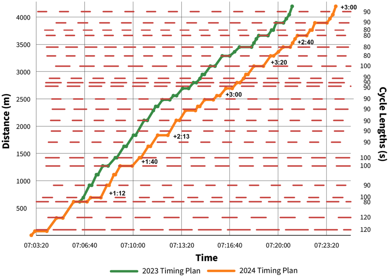
One-at-a-time analysis for traffic signal changes.
Figure 10 shows an observed trip before the timing plan change (green line). The Orange Line in the figure shows the potential impact on the trip travel time if we impose the same departure time, the same inter-stop time, and the same dwell time on the newly implemented signal timing plan with the red phases shown in red. The time deviations generated and the signal cycle lengths after the timing plan change are also marked on the graph.
Given the median observation before the timing plan change, the bus would complete the stop at the intersection around 614 m at 7:06:20. Checking the traffic signal timing plan, the light is green, and the bus can pass the intersection without any issue. Since the traffic lights are synchronized before the timing plan change, the bus would then proceed to pass the following intersections without any issue until reaching the stop and intersection at 1,270 m. However, given the change in timing plan, the signal is now red at this time, therefore the bus would wait until the green light comes on at 7:06:50, an additional 30 s. In addition, since the cycle lengths are now different, the signal would turn red as the bus arrives at the intersection. Therefore, the bus cannot immediately pass the intersection 75 m after, having to wait another 42 s for the red light. Given the extra 1 min and 42 s delay, the bus would miss the green light on the original cycle. When the next green light comes on, the bus will be 1 min 40 s or exactly one signal cycle late. However, since the intersection at 1,700 m received another cycle length change from 100 to 90 s, the bus is running one cycle and 10 s late. The light would remain green, but it is 10 s closer to the red light. However, as the bus approaches the signal at 1,900 m, the extra 10 s make it too late, and the bus must wait for another traffic light, further increasing the delay to 2 min and 13 s. Eventually, the bus could potentially arrive at the terminal two cycles later compared with the original timing plan given the chain-reaction effects.
From the figure, we can observe a potential 3-min increase in overall trip travel times as a result of the timing plan change. If we analyze the impacts locally at the spots with changed traffic signals, the difference between the two lines is only 1 min. However, this 1-min delay would cause the vehicle to potentially delay two additional minutes, because of missing more green lights later in the route. Also, from the figure, the bus very nearly misses a few signals after the changed signals. Thus, the inter-stop times or dwell times would also become more important if we consider the interaction effects. In reality, some drivers may drive fast to avoid hitting the red lights and some may slow down, which may or may not be the desired behavior. Again, planners want to look at the risks of hitting a red light at intersections and determine what they are going to plan for.
Once again, the cycle lengths are not necessarily the same on the entire route, and the signal timing plans were changed. Thus, the green waves are not aligned everywhere along the route. Planners must consider the potential chain-reaction effect after the signal changes to the end of the route rather than analyzing the impacts of traffic signal changes locally. Thus, we highlight once again the importance of including more detailed traffic signal configurations and interaction effects in the transit travel time studies.
For the three consecutive intersections used as an example in this section, a simple way to reduce the travel time variance could be to revert to using the same cycle length of 100 s. However, it is not quite possible to synchronize every traffic signal on every traffic corridor in the city, given the number of signalized intersections (around 2,600 in Montréal), various intersection configurations, and different travel demands. Synchronizing green waves for transit on a certain direction may also affect travel times for buses in the opposite direction. Transit planners must, therefore, work more closely together with traffic engineers to determine a better way to synchronize signals for buses and plan for travel times accordingly given these impacts. As mentioned by Furth et al. ( 7 ), the best way to improve transit travel time is to use both passive signal priority (i.e., setting traffic signals based on bus travel times) and active signal priority (i.e., based on real-time vehicle locations or sensor information).
Changing Departure Time
Sometimes buses did not leave at the intended time because of late arrivals from previous trips or waiting for a running passenger. Some agencies would also use algorithms to modify the departure times by a few minutes to facilitate interlining. However, one of the important variables discussed previously is the departure time, and it was shown to contribute a lot of variation to trip travel times and the red-light waiting times. Here, we use a median observation on the westbound Route 27 trip departing at 6:30 as an example to demonstrate the impacts of departure time by imposing the same inter-stop time, same dwell time at stops, and keeping the same traffic signal settings. The 6:30 departure has been moved around a few times to facilitate interlining by a few minutes during the past few years. Therefore, given the service frequency of 15 to 20 min, we will test a 15-min window for the departure time change as an example.
Figure 11 shows the trip travel time and red-light waiting time variations given various departure times. The times are calculated similarly to the previous two subsections, that is, updating the corresponding arrival and departure times as well as checking the signal timing plan to determine the signal state for all stops and signals. Therefore, we would not show the detailed calculations for length purposes. From the figure, we can observe that the trip travel time and red-light waiting time follow the same trend, which is not surprising as we kept the same inter-stop time and dwell times. This result shows a high correlation between the overall travel times and the overall red-light waiting times.
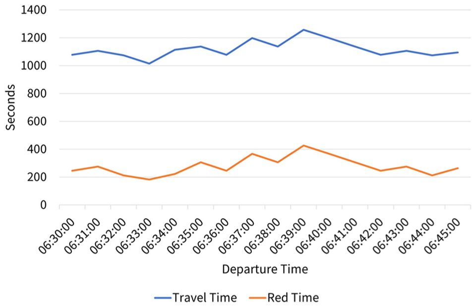
One-at-a-time analysis for departure time changes.
A 4-min difference can be observed on this 20-min route between 6:33 and 6:39 departures if we keep all other variables the same. As mentioned previously, the signal cycle lengths along this route are 80, 90, 100, and 120 s, with a least common multiple of 3,600 s. Thus, given any departure time within 1 h, the green wave patterns and the red-light waiting times will be different, resulting in large travel time and red-light waiting time variations shown above. Given the high correlation observed between the overall travel times and the red-light waiting times, we once again highlight the impact of departure time changes on the overall trip and red-light waiting times and the need for planners to plan carefully given the base signal timings.
Moreover, given that our on-time window is 4 min, small departure time changes on this route could also have a huge impact on the on-time performance. In addition, in reality, drivers may speed up to rush through the intersection before the light turns red (the interaction effects), which may or may not be a desired behavior. Therefore, planners need to carefully consider the consequences and add adequate schedule padding or layover times in case buses cannot depart on time for some reason. When optimizing for interlinings, the assumption that travel times remain constant if departure times are adjusted only by a few minutes is not necessarily a good assumption, as shown in this section. Therefore, planners might want to carefully select their departure times when adjusting schedules for interlining or adjusting service frequency to meet changing passenger demands. Alternatively, planners could also choose to settle on a fixed departure time, so that they will remain unchanged at a given anchor point (the peak load point for example). This way, planners could directly analyze the historical travel time observations without having to deal with the varying underlying green wave patterns.
Discussion
This section highlights the complex, non-linear relationships between individual trip elements, that is, dwell time, inter-stop time, traffic signal timing, and departure time. We also want to highlight once again the potential chain reaction and cumulative effects caused by individual element variations on the overall transit travel time.
Through one-at-a-time sensitivity analyses using a median trip observation from the westbound Route 27 during the morning peak, we demonstrate that small variations in any single factor can trigger significant downstream impacts, especially when interacting with the various states of traffic signals. Dwell and inter-stop time variations could be partially absorbed by red-light waiting time, unless a green phase is missed, leading to a significant increase in signal delays. Similarly, changes to traffic signal timing plans may break synchronization and create delays at intersections way past the changed sections. Even minor adjustments to departure time can potentially cause up to 4-min differences in travel time as a result of the variation in signal cycles. These findings underscore the need for transit planners to account for interaction effects and carefully select departure times when optimizing for interlining. Given the difficulty of synchronizing every traffic signal in the city, we want to emphasize the need for collaborations between transit planners and traffic engineers to optimize signal timing strategies and scheduling practices to improve travel time reliability safely for all road users.
Conclusions and Future Research
To summarize, transit reliability is important for both transit agencies and passengers. Larger travel time variations affect the scheduling process for transit agencies and trip planning decisions for passengers.
Previous studies mostly focused on either the variation of trip travel times or the variation of specific elements in trip travel times. The main focus on travel time variation has been on the contributing factors and the overall distribution of travel times. Dwell time variation has also been studied, though not directly related to the overall travel times. Traffic signal studies are mostly focused on giving priority to buses with mixed results. We identified that there is still a need to better isolate the variation in each trip element, further decompose the travel time, examine the interactions between these trip elements, and rank the impact of each element on the overall travel time variation.
Aiming to create more comprehensive evaluations of transit travel time variations and to help prioritize the resources for transit planners, we conducted both a variance-based sensitivity analysis and a one-at-a-time analysis for observed transit travel times. More specifically, we further decomposed 3 months of recorded transit travel times from 20 routes in Montréal into several trip elements, that is, departure time, inter-stop times, dwell times, and red-light waiting times. Departure time and inter-stop times can be obtained directly from the vehicle location data. However, because of the data limitation, the traffic signal settings and dwell times are estimated using various combinations of vehicle location data, fare transaction data, and ride-check observation data.
The results show that we can better decompose the travel times by adding more details on traffic signal settings and ridership variations, and that the variations in specific trip elements can be better isolated. The detailed data and sensitivity analyses allowed us to answer the question of where the travel time variances come from. The results for the 20 analyzed routes show that the overall travel time variations can come from all four elements identified, that is, departure time variations, inter-stop time (congestion) variations, dwell time (ridership) variations, and signal timing plan changes. However, as to how much variation can be attributed to each step, the results would vary at different time-of-day periods, from route to route, from segment to segment, and the interaction effects among different elements are very significant.
The most important element for half of the 20 routes analyzed in our case study is the departure time at the first stop, which determines how synchronized the traffic signals are further down the route, given the fixed coordinated timing plan with varying cycle lengths. In addition, most of the variation in the overall travel time and red-light waiting time came from the interaction effects, since red-light waiting times are the interaction effects of when the bus arrives at the signal and the signal timing plan. The inter-stop travel times and dwell times, however, are affected less by the interaction effects and can mostly be ranked by the individual variations. Therefore, areas with high ridership and congestion variations tend to have high impacts on the overall travel time as expected. The one-at-a-time analysis also demonstrated the non-linear relationship between the variation of each trip element and the trip travel time variation.
Planners need to choose the departure time carefully and better understand the base signal timings before designing or adjusting service schedules. Slightly modifying the departure time to facilitate interlining is not necessarily a good idea without a better understanding of the potential impact on the overall travel times. As we demonstrated, the historical vehicle location and travel time observations are conditional given the fixed signal plan and the varying cycle lengths. A slight change in departure time can potentially cause a large travel-time variation as a result of the changes in signal synchronization patterns. Planners could either optimize for specific departure times rather than applying the same travel time everywhere, or add adequate schedule padding to account for the travel time variations, which would increase operating costs. Similarly, small changes in signal timing plan changes can have a chain-reaction effect on the overall travel times. The travel time variations in the affected area can be small, but the impact on the whole trip can be large because of the interaction effects. Thus, planners need to include more detailed signal timing plans and red-light waiting time information when scheduling or planning for transit travel times.
To conclude, we want to again highlight our contribution in the data integration, which includes common data sources widely available to the agencies, as well as the analysis scale, which is more detailed compared with the existing studies. Since the current literature tends to focus on one specific aspect of travel time, our research also adds to the literature on how to combine these different elements in a more comprehensive study and how these different elements interact. The basic framework and the results help identify important determinants for travel time variations for practitioners and future research directions for researchers.
However, there are many limitations and potential future research areas that are needed. The first is related to our analysis scale. We have only analyzed three months of recent data, yet we would need more observations to better reduce the confidence intervals for less frequent routes during off-peak times. There is also a need for a longitudinal study to discover potential trends and changes in the sensitivity results to better inform transit planners on the changes in the system. With more data on more routes, it will also be possible to examine potential temporal and spatial patterns affecting transit travel time reliability, which may in turn help the planning process for new schedules or routes.
Our methodology does not currently consider the interaction between buses, since delays can affect the number of boardings and alightings, where the vehicle may pick up additional passengers that are supposed to take the following vehicle. Our methodology also only considers the overall dwell time variations within a time-of-day period without considering detailed overall passenger flow variations and the impacts on travel times. Unfortunately, as a result of the data limitations, we cannot carry out a more detailed ridership analysis or estimate a more comprehensive model here to include the overall passenger flow, various day-to-day ridership variations, and seasonal ridership patterns. Similarly, there are various studies on the interaction of bus bunching, irregular headways, and ridership variations ( 24 ), yet there is still a need to incorporate these vehicle and ridership interactions into the various variance analysis models to determine the interaction effects and reliability impacts of these factors. In addition, although there is some research on the passenger arrival rates ( 25 ), it is not easy to determine the passenger arrival rates at bus stops using the fare collection data available to us, nor to add this information into variance decomposition models. As the agency in the region improves the ridership matching algorithm, some of these limitations could be addressed by future researchers. By incorporating this information, future researchers could improve the accuracy of the travel time models, better pinpoint issues on the routes, and better inform planning and operation decisions.
In addition, since our traffic signals mainly use fixed timing plans with very little flexibility for transit signal priorities, there is a need to better understand the interaction between buses and non-fixed timing signals using empirical data, as the majority of the current literature is based on simulations. This way, we could potentially compare various transit systems to identify pros and cons in various configurations to help improve transit reliability. Similarly, future research could find a better way to give signal priority to buses in traveling down a coordinated corridor with densely configured signals.
Footnotes
Acknowledgements
The authors would like to thank the Société de Transport de Montréal and Autorité Régionale de Transport Métropolitain for providing data access.
Author Contributions
The authors confirm contribution to the paper as follows: study conception and design: Yuxuan Wang, Catherine Morency, Martin Trépanier; data collection: Yuxuan Wang, Catherine Morency, Martin Trépanier; analysis and interpretation of results: Yuxuan Wang, Catherine Morency, Martin Trépanier; draft manuscript preparation: Yuxuan Wang, Catherine Morency, Martin Trépanier. All authors reviewed the results and approved the final version of the manuscript.
Declaration of Conflicting Interests
The authors declared no potential conflicts of interest with respect to the research, authorship, and/or publication of this article.
Funding
The authors disclosed receipt of the following financial support for the research, authorship, and/or publication of this article: This research is funded by the Natural Science and Engineering Research Council of Canada through Discovery Grants RGPIN-2024-04806 and RGPIN-2024-06797, and the Canada Research Chair in Transportation Transformation.
Data Accessibility Statement
Most of our research data are freely available online, such as the GTFS, GTFS-RT, and OpenStreetMap files. Researchers can access the most up-to-date versions directly from the related websites. The archived GTFS data, GTFS-RT data, and the code used in the study can be provided on reasonable request to the authors. As we continue to improve the precision of our estimates and algorithms, we do not guarantee that the exact values will remain unchanged. However, we cannot provide the fare transaction data because of potential privacy issues in accordance with our data agreement with the transit agencies.