Enhancing Travel Mode-Choice Modeling with Route-Based Attributes and Explainable Machine Learning

Abstract

Modeling mode choice is essential for designing efficient and sustainable mobility systems. Revealed-preference surveys provide valuable information, but they rely on self-reported data, which can be biased and are typically unavailable for unchosen alternatives. This study proposes an integrated analytical process that combines revealed-preference survey data, route-level attributes derived from a digital trip planner, machine-learning classifiers, and explainable artificial intelligence (XAI) methods to evaluate predictive performance and behavioral interpretation jointly. Using a dataset of 1,372 trips collected in a university commuting context as an illustrative application, survey responses were enriched with mode-specific travel times and geometric characteristics of planner-recommended routes obtained from Google Maps’ application programming interface. Four tree-based classifiers were evaluated in a leak-free validation framework, and model behavior was interpreted using SHAP (SHapley Additive exPlanations) and LIME (Local Interpretable Model-agnostic Explanations) at both the global and local levels. The results indicate that when route-level geometric attributes were combined with revealed-preference survey data, predictive accuracy remained comparable, whereas interpretability improved substantially. XAI analyses revealed that route characteristics such as straightness, sinuosity, and angular deviation emerged as significant predictors that modulated perceived travel effort, particularly for walking and public transport, despite their limited impact on aggregate performance.

Keywords

revealed preferences (RP)machine learning (ML)XAI methods (SHAP LIME)route characterization passive data

Introduction

Understanding travel mode choice is fundamental to the design of transportation systems. Mode choice reflects the process by which individuals select a transport alternative for a given trip based on attributes such as travel time, cost, comfort, and accessibility. Accurate models of mode-choice behavior are therefore essential for urban planning, infrastructural investment, environmental policy-making, and the promotion of equitable mobility outcomes.

Traditionally, travel mode choice has been analyzed using revealed-preference (RP) surveys, which record observed travel behavior including trip origins and destinations, chosen modes, trip purposes, and self-reported travel times. These data are often complemented with sociodemographic characteristics. RP surveys remain a cornerstone of travel behavior research because they reflect real-world decisions made under actual constraints. However, they also present well-known limitations, particularly their reliance on self-reported attributes, which are susceptible to recall bias, rounding, and subjective perception errors.

In recent years, the increasing availability of passively collected mobility data has opened up new opportunities to enrich traditional survey-based analyses. Data sources such as GPS traces, smartphone applications, and digital route planners offer high spatial and temporal resolution with relatively low respondent burden, and have been used to complement or validate survey information in travel behavior studies ( 1 , 2 , 3 ). Among these sources, digital travel planners such as Google Maps are particularly attractive, as they provide standardized, network-constrained estimates of travel times, distances, and routes across multiple modes for the same origin–destination (OD) pair.

A common motivation for using planner-derived data is to mitigate biases in self-reported data by replacing them with more objective measures ( 4 , 5 , 6 ). However, travel planners provide more than just travel-time estimates. By generating explicit routes that reflect network structure, connectivity, and mode-specific constraints, they also enable the extraction of route-level geometric attributes, such as straightness and directional variability. These measures describe the complexity and directness of feasible paths through the transport network ( 7 ) and capture dimensions of travel that are not fully summarized by travel time.

A growing body of literature suggests that such geometric and network-based attributes influence travel behavior through multiple mechanisms. Route directness and straightness have been linked to perceived effort, comfort, safety, and cognitive load, particularly for walking and cycling. Frequent directional changes, detours, and fragmented street networks can increase perceived travel burden even when travel times remain comparable ( 8 ). More broadly, research on street network configuration and centrality shows that urban form shapes accessibility, movement patterns, and land-use interactions, which in turn influence mobility choices across population groups ( 9 ). Collectively, these studies underscore the role of street configuration and network complexity in shaping travel behavior.

Despite this evidence, route-level geometric attributes remain underutilized in travel mode-choice modeling, particularly in conjunction with modern machine-learning methods. Discrete choice models, and especially the multinomial logit (MNL) model ( 10 ), have long been the dominant analytical framework owing to their strong behavioral foundations and interpretability. However, their performance and flexibility depend on the correct specification of functional forms and interactions. Motivated by increasing data richness and computational power, recent studies have explored machine-learning algorithms such as random forests (RFs), gradient boosting, and neural networks (NNs) for mode-choice modeling ( 11 , 12 , 13 ). These models can flexibly capture nonlinear relationships and complex interactions that are difficult to specify a priori in parametric settings.

At the same time, the adoption of machine-learning methods in transportation research has raised concerns with regard to interpretability and transparency. Complex nonparametric models are often criticized for their limited explanatory power in policy and planning contexts. To address this challenge, explainable artificial intelligence (XAI) methods such as SHAP (SHapley Additive exPlanations) ( 14 ) and LIME (Local Interpretable Model-agnostic Explanations) ( 15 ) have gained increasing attention. These tools provide global and local explanations of model predictions, enabling researchers to assess variable importance, effect direction, and individual-level decision logic in a transparent manner.

Against this backdrop, this study advances the analysis of travel mode choice by explicitly integrating route-level geometric characterization into a data-driven and explainable modeling framework. Rather than treating planner-derived travel times as a direct replacement for self-reported measures, we argue that geometric properties of network-constrained routes capture complementary dimensions of perceived travel effort and route quality that may influence mode-choice behavior across alternatives.

To operationalize this idea, we propose an end-to-end analytical pipeline that combines RP survey data, standardized route characterization derived from a digital travel planner, machine-learning classifiers, and XAI techniques. Using a university travel context as an illustrative application, we assess not only whether planner-derived attributes improve predictive performance, but also how they reshape the explanatory structure of mode-choice models. In doing so, the study contributes a transparent and transferable methodology for extracting behavioral insight in contexts where large-scale passive mobility datasets are unavailable but routing services can provide consistent network-based proxies at low cost.

The rest of this article is structured as follows. The section on related works presents a brief review of the literature. The methods section describes the methodology, followed by the description and results of the datasets of empirical application. Finally, the discussion and conclusions section closes the paper with concluding remarks, identifying the limitations of the article and suggesting future research directions.

Related Works

Travel mode choice has long been a central topic in transportation research, as understanding how individuals select among available transport alternatives is essential for effective planning, policy design, and system management. Early and foundational work in this area has predominantly relied on discrete choice models grounded in random utility maximization theory ( 16 ). Among these, the MNL model introduced by McFadden remains the most widely applied owing to its analytical tractability and clear behavioral interpretation ( 10 ). Numerous empirical studies have successfully employed MNL and its extensions to explain modal decisions across diverse contexts (e.g., 17, 18, 19, 20).

Despite their strong theoretical foundations, discrete choice models are sensitive to data quality and model specification. In particular, their explanatory and predictive performance depends on the accurate measurement of attributes for all available alternatives and on correctly specified functional forms. These limitations have motivated sustained interest in expanding data sources beyond traditional surveys and in exploring alternative modeling approaches capable of capturing more complex relationships.

RP and stated-preference (SP) surveys have traditionally formed the empirical backbone of mode-choice analysis. RP surveys document observed behavior under real-world constraints, whereas SP surveys allow researchers to explore hypothetical scenarios and policy interventions ( 21 , 22 ). Although both approaches have contributed substantially to the literature, they are not without drawbacks. RP surveys often lack reliable information for unchosen alternatives, whereas SP surveys may suffer from hypothetical bias and cognitive burden. In addition, both approaches typically rely on self-reported travel times and distances, which are prone to recall and perception errors.

The increasing availability of passive and semipassive mobility data has opened up new avenues to address some of these limitations. As highlighted by Tsoleridis et al., emerging data sources such as GPS traces, smartphone sensors, and digital route planners provide high-resolution spatial and temporal information with relatively low respondent burden ( 3 ). Among these, map-service application programming interfaces (APIs) have gained particular attention owing to their ability to generate standardized, network-constrained travel times, distances, and routes across multiple modes.

Several studies have leveraged these technologies to support transport analysis and planning. For example, Liu et al. combined Baidu Map API data with geographic information system techniques to evaluate accessibility and spatial equity in school placement ( 23 ), whereas Ha et al. employed a route guidance API to assess the role of travel time and cost in modal decisions in Seoul ( 24 ). Other contributions have integrated Google Maps API into survey instruments to collect OD coordinates and reconstruct routes, enabling more detailed mobility profiling ( 21 ). These studies demonstrate the potential of planner-derived data to enrich traditional datasets, particularly where direct observation of routes or times is unavailable.

Beyond travel-time estimation, route planners enable the extraction of route-level geometric and network attributes that characterize the structure and complexity of feasible paths. A growing body of literature suggests that such attributes influence travel behavior through mechanisms that extend beyond generalized cost. Studies on route choice have shown that travelers often prefer more direct routes, avoid frequent turns, and respond to the configuration of the street network ( 25 ). From a cognitive perspective, route complexity, directional changes, and network fragmentation can increase perceived effort and navigational burden, particularly for active modes ( 8 ).

More broadly, research on street network configuration and centrality has highlighted how urban form shapes accessibility, movement patterns, and land-use interactions. Measures such as straightness, betweenness, and closeness centrality have been linked to mobility flows, land-use intensity, and spatial equity, underscoring the role of network structure in shaping travel opportunities ( 9 ). These insights suggest that route-level geometric attributes may act as proxies for perceived route quality and network impedance, even when travel times are held constant.

Despite this evidence, such attributes remain relatively underexplored in travel mode-choice modeling, especially when combined with flexible, data-driven methods. Most existing studies that use planner-derived data focus primarily on travel times and costs, with limited attention paid to how route geometry may systematically influence modal decisions.

In parallel with the expansion of available data, machine-learning methods have been increasingly adopted in mode-choice analysis. Algorithms such as RFs, gradient boosting, NNs, and support vector machines have been shown to outperform classical discrete choice models in predictive accuracy in several empirical applications (12, 26, 27 , 28 ). These methods are particularly well suited to capturing nonlinear relationships and high-order interactions among explanatory variables, which are difficult to specify a priori in parametric frameworks.

Recent studies have further enriched ML-based mode-choice models by incorporating external data sources, including planner-derived travel times and costs ( 28 ), smartphone sensor data ( 29 ), and spatial features extracted from GPS trajectories ( 30 ). Although these approaches demonstrate the predictive potential of ML, they also raise concerns about transparency and behavioral interpretability, especially in policy-oriented contexts.

To address these concerns, XAI techniques such as SHAP ( 14 ) and LIME ( 15 ) have been increasingly adopted in transportation research. In the context of mode choice, XAI methods have been used to identify influential variables, assess heterogeneity in responses, and generate individual-level explanations of model predictions ( 31 , 32 , 33 ). Beyond mode choice, interpretable ML has been applied to crash analysis, spatiotemporal risk prediction, and traffic control, highlighting its broader relevance for actionable decision support in transportation systems ( 34 , 35 ).

Moreover, prior studies that exploit digital travel planners have primarily emphasized the use of API-derived travel times and costs as more objective substitutes or complements to self-reported measures. For instance, Kelly et al. ( 6 ) and Houston et al. ( 5 ) focus on discrepancies between reported and observed travel times, highlighting perception and recall biases while treating planner-based times as benchmark indicators. Similarly, Ha et al. ( 24 ) integrates routing information from a navigation API to improve the measurement of modal attributes, but the analysis remains centered on travel time and cost effects. More recently, Martín-Baos et al. (36) enriched a large-scale mode-choice dataset with API-based travel times and costs to enhance ML performance, yet the planner-derived information is again interpreted mainly through generalized cost proxies ( 28 ).

In parallel, a distinct body of literature in route choice, spatial cognition, and urban network analysis has shown that route-level properties such as directness, connectivity, and directional complexity influence perceived travel effort and movement patterns. Early experimental work by Montello ( 8 ) demonstrates that path complexity affects cognitive distance and navigation effort ( 8 ), whereas empirical evidence from GPS-based studies indicates preferences for routes with fewer turns and greater directness ( 25 ). At a broader urban scale, network-based measures of street configuration and centrality have been shown to shape accessibility and mobility outcomes across population groups ( 9 ). Table 1 provides an overview of travel mode-choice studies, classified according to data type, modeling approach, and use of XAI techniques.

Table 1.

Overview of Travel Mode-Choice Studies, Classified According to Data Type (Revealed and Stated Preferences, Passive Data), Modeling Approach (Discrete Choice Models and Machine-Learning Algorithms), and Use of Explainable Artificial Intelligence Techniques. Checkmarks Indicate the Explicit Inclusion of Each Methodological Component in the Corresponding Study

Authors	Year	ML models	DCM models	RP	SP	Passive	ML	XAI	Journal
Jahangiri and Rakha [37]	2015	KNN, SVM, RF	na			✓	✓		IEEE-TITS
Tang et al. [38]	2016	DT	MNL	✓			✓		TPT
Sekhar and Madhu et al. [39]	2016	RF	MNL	✓			✓		TRP
Hagenauer and Helbich [12]	2017	NB, SVM, NN	MNL	✓			✓	✓	ESWA
Wang and Ross [40]	2018	XGB	MNL	✓		✓	✓		TRR
Lee et al. [41]	2018	NN	MNL	✓			✓		TRR
Cheng et al. [42]	2019	RF, SVM, AdaBoost	MNL	✓	✓		✓		TBS
Sifringer et al. [43]	2020	NN	MNL		✓		✓		TR-B
Zhao et al. [44]	2020	NB, RF, SVM, NN	MNL, MMNL		✓		✓		TBS
Li et al. [30]	2020	CNN, SVM, ANN, RF	na			✓	✓		TR-A
Liu et al. [23]	2020	na	na			✓			IJGI
Wong and Farooq [45]	2021	NN	MNL	✓			✓		TR-C
Kim [46]	2021	XGB, RF, ANN	na	✓			✓	✓	JAT
Han et al. [47]	2022	NN	MNL		✓		✓		TR-B
Kashifi et al. [48]	2022	RF, LR, DT, MLP	MNL	✓			✓	✓	TBS
Salas et al. [27]	2022	KNN, NN, SVM, XGB	MNL, MMNL	✓	✓		✓	✓	ESWA
Liu et al. [49]	2023	NN	ICLV		✓		✓		JCM
Martín-Baos et al. [36]	2023	NN, RF, XGB	MNL	✓			✓		TR-C
Ren et al. [50]	2023	XGB	MMNL	✓			✓		Transportation
Xia et al. [51]	2023	NN, BNN	MNL	✓			✓		TBS
Díaz-Ramírez et al. [52]	2023	XGB, RF, DT, SVM	na	✓			✓		CEI
Arkoudi et al. [53]	2023	NN	MNL	✓	✓		✓		TR-B
Yang et al. [54]	2024	RF	na			✓	✓	✓	TBS
Sarker et al. [33]	2024	XGB	na		✓		✓	✓	MT

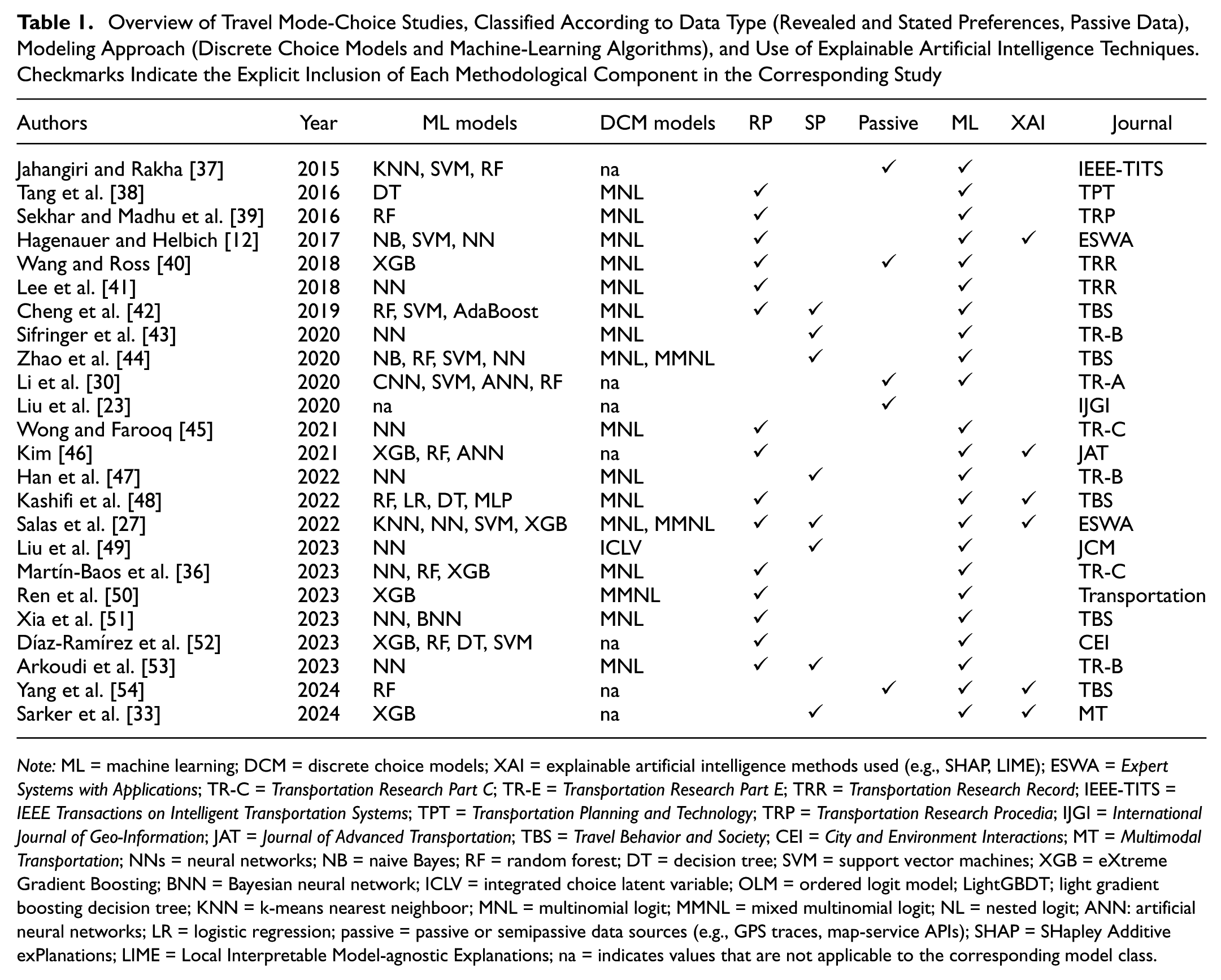
Note: ML = machine learning; DCM = discrete choice models; XAI = explainable artificial intelligence methods used (e.g., SHAP, LIME); ESWA = Expert Systems with Applications; TR-C = Transportation Research Part C; TR-E = Transportation Research Part E; TRR = Transportation Research Record; IEEE-TITS = IEEE Transactions on Intelligent Transportation Systems; TPT = Transportation Planning and Technology; TRP = Transportation Research Procedia; IJGI = International Journal of Geo-Information; JAT = Journal of Advanced Transportation; TBS = Travel Behavior and Society; CEI = City and Environment Interactions; MT = Multimodal Transportation; NNs = neural networks; NB = naive Bayes; RF = random forest; DT = decision tree; SVM = support vector machines; XGB = eXtreme Gradient Boosting; BNN = Bayesian neural network; ICLV = integrated choice latent variable; OLM = ordered logit model; LightGBDT; light gradient boosting decision tree; KNN = k-means nearest neighboor; MNL = multinomial logit; MMNL = mixed multinomial logit; NL = nested logit; ANN: artificial neural networks; LR = logistic regression; passive = passive or semipassive data sources (e.g., GPS traces, map-service APIs); SHAP = SHapley Additive exPlanations; LIME = Local Interpretable Model-agnostic Explanations; na = indicates values that are not applicable to the corresponding model class.

Despite these insights, route-level geometric attributes have rarely been incorporated into ML-based mode-choice models, nor systematically examined through XAI tools. Consequently, little is known about how such attributes contribute to, or reshape, the explanatory structure of ML models, particularly in cases where their inclusion does not yield substantial gains in aggregate predictive performance.

This study addresses these gaps by proposing an end-to-end analytical pipeline that combines RP surveys, standardized route characterization from a digital travel planner, ML classifiers, and XAI techniques. By focusing jointly on predictive assessment and interpretability, the proposed framework advances current practice and provides a transferable methodology for extracting behavioral insight from enriched mobility data in data-constrained planning contexts.

Methods

Travel Planner–Derived Attributes

Travel planners based on digital mapping services provide route-level information such as travel times, distances, and network-constrained paths between OD pairs. In this study, we use the Google Maps Directions API to derive mode-specific travel attributes for each reported trip, thereby augmenting the RP survey with standardized, planner-based information.

For each OD pair, the API returns a recommended route for each available travel mode, computed according to mode-specific routing criteria embedded in the service. The retrieved information includes estimated travel time, distance, and the polyline geometry of the suggested route. The following modes are considered:

Cycle: Routes and travel times computed based on the available cycling infrastructure and cycling-specific network constraints.

Walk: Pedestrian routes optimized for shortest feasible walking paths, accounting for sidewalks, crossings, and pedestrian accessibility.

Transit: Public transport (Hamilton Street Railway—local bus) routes including access to stops, in-vehicle travel time, transfers, and service availability within the local transit network.

Car: Driving routes and travel times computed under prevailing traffic assumptions embedded in the routing engine.

Travel times obtained from the Google Maps API are inherently dependent on routing assumptions and prevailing network conditions, including time-of-day and congestion levels ( 1 ). In this study, API-derived travel times are therefore not interpreted as exact counterfactuals of experienced travel time at the moment of survey completion. Instead, they are treated as standardized, network-based proxies of relative travel effort across alternatives, computed under a consistent query protocol. This approach ensures internal comparability across modes and observations while acknowledging the absence of perfect temporal alignment between survey-reported trips and planner-based estimates.

Route Characterization

To enrich the analysis of travel mode choice, spatial data processing tools were used to extract detailed information from the routes suggested by the travel planner for each OD pair and travel mode. These routes correspond to standardized, network-constrained alternatives generated under mode-specific routing criteria, rather than observed or realized travel routes.

Route-level geometric variables are incorporated to characterize the structure and quality of the feasible alternatives available to travelers across modes, drawing on the growing use of passive and semipassive data sources in transport analysis ( 3 ). Rather than describing ex post behavior, these attributes capture properties of the transport network and of the planner-generated paths that may shape perceived travel effort and relative attractiveness at the time of choice.

Accordingly, the indicators computed in this study summarize route directness, geometric complexity, and directional variability embedded in the routing engine’s network representation. They serve as reproducible proxies for relative travel impedance across modes and complement self-reported travel attributes with internally consistent, planner-derived information.

The following route-level indicators were computed for each travel mode based on the routes obtained from the Google Maps API (see Figure 1):

Straightness: A geometric indicator of route directness defined as the ratio between the straight-line (Euclidean) distance and the actual route length. Higher values denote more direct paths, whereas lower values indicate increased deviation and geometric complexity ( 55 ).

Maximum angular deviation (Emax): The largest angular deviation of any route segment from the straight line connecting origin and destination. Higher values indicate sharper turns or major deviations.

Mean directional change: The average change in direction between consecutive segments, reflecting route smoothness ( 56 ).

Standard deviation of directional change: Measures variability in angular changes, with higher values indicating more erratic routes ( 56 ).

Data processing was conducted using the R software environment, employing libraries such as ggmap ( 57 ) for map visualization and geocoding. Functions like revgeocode were used to transform coordinates into addresses, whereas mapdist calculated distances and travel times. Additionally, the trek and trajr packages ( 58 ) facilitated the extraction and computation of route characteristics.

Figure 1.

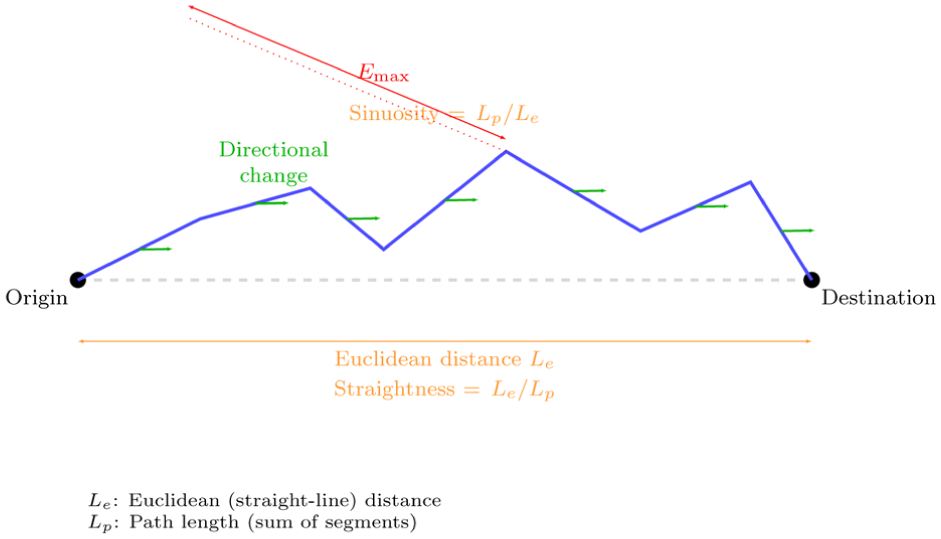
Geometric and directional properties of routes.

Machine-Learning Algorithms

Mode choice was formulated as a multiclass classification task. We benchmarked four tree-based learners that jointly offered strong accuracy, modest tuning effort and compatibility with explanations methods:

A single classification and regression tree (CART) ( 59 );

The bagging ensemble RF ( 60 ), which averages many decorrelated trees to reduce variance;

The sequential-boosting ensemble Adaptive Boosting (AdaBoost) ( 61 ), which reweights misclassified observations at each iteration; and

The gradient-boosting powerhouse eXtreme Gradient Boosting (XGBoost) ( 62 ), whose shrinkage and column-subsampling refinements usually deliver the best accuracy.

Bagging methods such as RF build trees independently on bootstrap samples, whereas boosting methods (AdaBoost, XGBoost) grow trees sequentially so that each learner corrects the residual errors of its predecessors ( 63 , 64 ). RF is robust to noisy, nonlinear relationships with minimal tuning, whereas XGBoost achieves state-of-the-art results at the cost of more hyperparameters.

Hyperparameter optimization is performed exclusively on the training data using stratified $K$ -fold cross-validation. Within each fold, the model is trained on the corresponding training partition and evaluated on the validation partition, preserving the class distribution across folds. All preprocessing steps—including imputation, categorical encoding, and class imbalance handling—are embedded within a unified pipeline and are applied only to the training portion of each fold, ensuring a strictly leakage-free tuning process. Table 2 presents the hyperparameters associated with each algorithm.

Bayesian optimization is conducted with a fixed budget of 30 iterations per model, and hyperparameters are selected by maximizing the mean macro $F_{1}$ -score computed under a repeated stratified $5 \times 5$ cross-validation scheme. For transparency and robustness assessment, cross-validation results are summarized as mean ± standard deviation of the evaluation metric and reported in Table 6.

Performance estimates obtained during cross-validation are used solely for hyperparameter selection. The final evaluation is conducted separately on a held-out test set that is not involved in any stage of preprocessing or tuning. All experiments were implemented in Python using the scikit-learn ecosystem, with fixed random seeds to ensure full reproducibility.

Evaluation Metrics

Model performance was assessed using standard classification metrics computed from the confusion matrix: overall accuracy, recall, and $F 1$ -score. Let $n_{ij}$ represent the number of observations belonging to class $i$ that are predicted as class $j$ , and $n_{ii}$ the correctly classified observations in class $i$ . The confusion matrix enables the computation of

Accuracy (first preference recovery),

Acc = \frac{\sum_{i = 1}^{J} n_{ii}}{\sum_{i = 1}^{J} N_{i}},

(1)

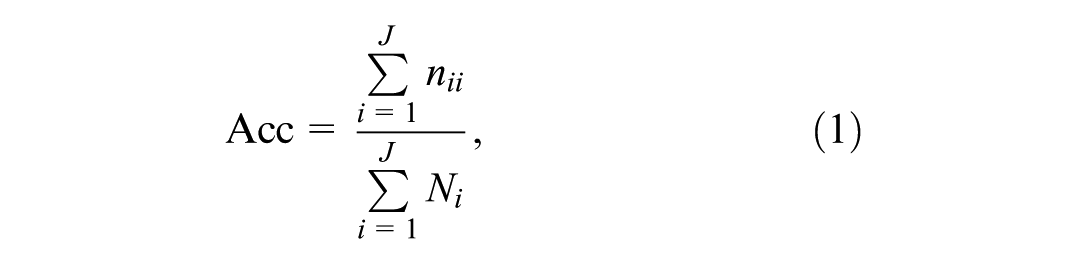
where $N_{i} = \sum_{j = 1}^{J} n_{ij}$ is total number of observations in class $i$ .

Recall (per class),

Recal l_{i} = \frac{n_{ii}}{N_{i}},

(2)

measuring the proportion of correctly identified observations within class $i$ .

$F 1$ -score (per class),

F 1_{i} = 2 \cdot \frac{Precisio n_{i} \cdot Recal l_{i}}{Precisio n_{i} + Recal l_{i}},

(3)

where $Precisio n_{i} = n_{ii} / \sum_{j = 1}^{J} n_{ji}$ .

Explainable Artificial Intelligence (XAI) Methods

Tree ensembles offer high predictive power at the expense of interpretability. We therefore complement the performance analysis with two model-agnostic, post hoc explanation tools that are now standard in transport applications: TreeSHAP for global attributions and LIME for case-specific diagnostics.

Within this methodological context, our study leverages SHAP and LIME to interpret how planner-derived passive data and route-level geometric attributes contribute to travel mode choice. Although SHAP provides a global view of variable importance and directional effects across the population, LIME offers complementary local explanations that illustrate how these attributes interact at the individual level. This combined perspective is particularly relevant for planning contexts where traditional passive mobility data sources are limited or unavailable.

SHapley Additive exPlanations (SHAP)

SHAP attributes the prediction of a complex model to individual variables based on Shapley values from cooperative game theory ( 14 , 65 ).

For a given observation, the original model, $f$ , is locally approximated by an additive surrogate of the form

g (z^{'}) = ϕ_{0} + \sum_{j = 1}^{M} ϕ_{j} z_{j}^{'},

(4)

where $z_{j}^{'} \in {0, 1}$ denotes whether variable $j$ is included in the coalition, and $ϕ_{j}$ represents its marginal contribution to the model output.

For tree-based ensembles, the TreeSHAP algorithm computes these contributions in polynomial time while satisfying key axiomatic properties, including local accuracy and consistency ( 14 ). Global variable importance is assessed using the mean absolute SHAP value, $| ϕ_{j} |$ , across all observations, and summary beeswarm plots are used to visualize both the magnitude and direction of variable effects.

In the multiclass setting, TreeSHAP is applied to explain the raw outputs of the XGBoost model, corresponding to the latent class scores before the softmax transformation. Accordingly, positive (negative) SHAP values indicate that a given attribute increases (decreases) the latent score of a specific travel mode, thereby enhancing (reducing) its relative competitiveness within the multinomial decision framework, rather than directly affecting predicted probabilities.

Local Interpretable Model-agnostic Explanations (LIME)

Whereas SHAP provides a global-level view, LIME explains a single prediction by fitting a simple interpretable model, $v \in V$ , in the vicinity of the instance of interest, $x$ ( 15 ). The weights of $v$ are estimated by minimizing

\underset{v \in V}{argmin} ℓ (f, v, π_{x}) + Ω (v),

(5)

where $π_{x}$ is a locality kernel and $Ω (v)$ penalizes model complexity ( 66 ). We generate perturbations per decision maker and report the 10 most influential variables, thereby revealing the specific route or socioeconomic conditions that drive an individual predicted mode choice.

Application

Original RP Dataset

The student travel dataset originates from a survey conducted at McMaster University (Hamilton, Canada) by Whalen et al. ( 20 ). Building on that instrument, an online RP survey was administered in autumn 2019 to capture current student travel behavior. The questionnaire recorded the geographic coordinates of the trip origin (home) and the regular mode for the home–campus journey; self-reported travel time for the chosen mode; socioeconomic attributes such as age, gender, household type and vehicle ownership; and attitudinal reasons underlying the stated choice. After data cleaning, the final sample comprised $1, 372$ valid responses.

The dependent variable was the student’s modal choice, with four alternatives: cycling, walking, transit and car. Walking was the dominant alternative in the sample, whereas cycling was clearly underrepresented (see Table 4). The complete list of original variables considered in the modeling is provided in Table 3.

Table 2.

Hyperparameter Search Space for Each Classifier Used in Bayesian Optimization

Algorithm	Hyperparameter description	Python argument	Search range
CART	Function to evaluate split quality	criterion	{gini, entropy}
	Maximum tree depth	max_depth	{1, 2 …, 20}
	Maximum number of features	max_variables	{sqrt, log2}
RF	Function to evaluate split quality	criterion	{gini, entropy}
	Maximum tree depth	max_depth	{1, 2 …, 20}
	Number of trees in the forest	n_estimators	{100, …, 500}
	Maximum number of features	max_variables	{sqrt, log2}
XGB	Maximum tree depth	max_depth	{1, 2,…, 20}
	Learning rate	learning_rate	[0.05, 0.31]
	Number of boosting rounds (trees)	n_estimators	{100, …, 500}
	Minimum loss reduction to split (gamma)	gamma	[0, 0.5]
	Minimum child weight	min_child_weight	{1, 2,…, 10}
	Subsample ratio for each tree	subsample	[0.7, 1]
	P column-subsampling ratio per tree	colsample_bytree	[0.7, 1]
AdaBoost	Learning rate	learning_rate	[0.05, 0.31]
AdaBoost	Number of estimators (weak learners)	n_estimators	{100, …, 500}

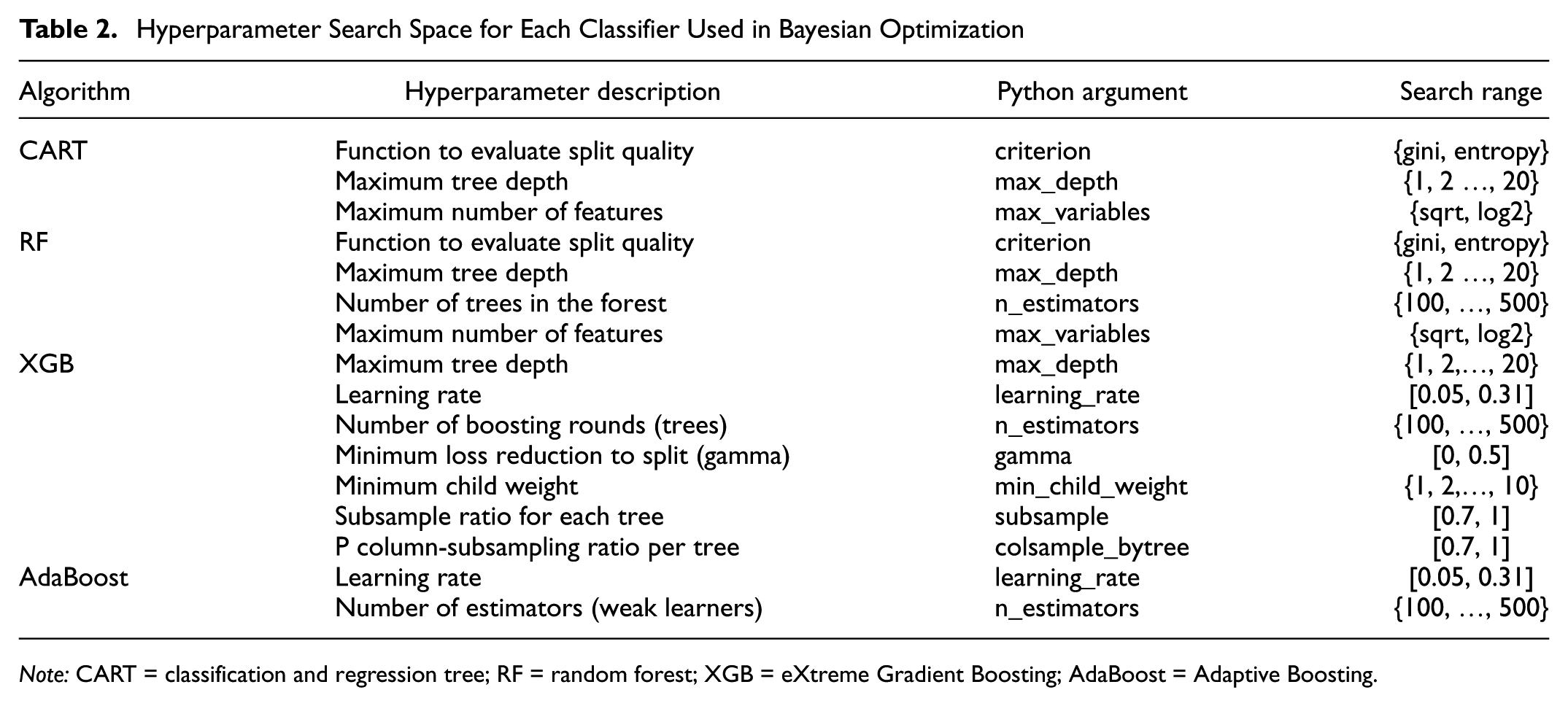
Note: CART = classification and regression tree; RF = random forest; XGB = eXtreme Gradient Boosting; AdaBoost = Adaptive Boosting.

Table 3.

Attributes Definition

Source	Code	Description
Survey	time	Self-reported travel time for each mode (min)
	access_Transit	Walk time to nearest transit stop (min)
	street_density	Street length per km²
	sidewalk_density	Sidewalk length per km²
	parking	Campus parking permit available (1 = yes)
	shelter_A	High-quality transit shelter within $250$ m
	shared	Shared accommodation (1 = yes)
	solo	Single accommodation (1 = yes)
Passive	TT_mode	Google trip time for each mode (min)
	straightness	$d_{eucl} / L$ (ratio)
	sinuosity	$100 \times L / d_{eucl}$ (%)
	Emax	Maximum angular deviation from origin–destination bearing (°)
	mean_dir	Mean directional change between segments (°)
	sd_dir	SD of directional change (°)

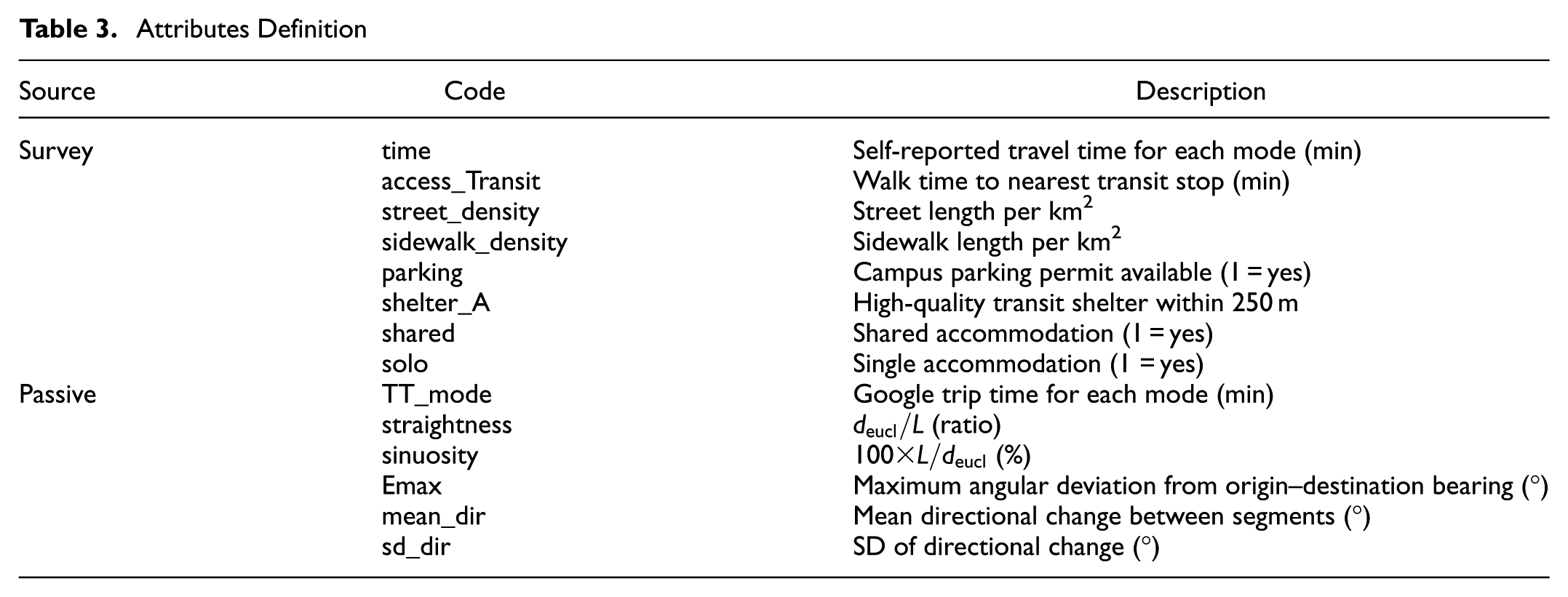
All explanatory variables employed in the modeling—together with descriptive statistics—are listed in Table 4. Because the survey only asked respondents to report attributes of the mode they actually used, many alternative–specific variables are missing. The observations displayed a clearly clustered spatial pattern around the campus, thinning out with distance (Figure 2). By mode, walk origins are concentrated within a smaller radius around the destination; cycle aligned with corridors near the bikeway network and finer street connectivity; transit followed major bus arterials and transfer nodes; and car exhibited a more diffuse, peripheral footprint. Taken together, these gradients mirrored the interplay between transport supply and urban form: areas with strong pedestrian accessibility and frequent transit service skewed toward sustainable modes, whereas lower-access, farther-flung zones showed a higher incidence of car trips.

Table 4.

Descriptive Statistics of the Variables of the “Student Travel at McMaster University” Dataset, Including Passive Data-Derived Attributes

Mode	Cycle				Car				Transit				Walk
Share (%)	48 (3.5)				280 (20.4)				333 (24.3)				711 (51.8)
Original numerical variables	Min.	Max.	Mean	SD	Min.	Max.	Mean	SD	Min.	Max.	Mean	SD	Min.	Max.	Mean	SD
Travel time (min)	0.29	45.00	6.40	5.11	1.00	72.00	9.17	9.35	1.00	120.00	16.29	20.21	1.00	62.11	18.05	11.41
Street density (km/km²)	4.2	19.5	13.5	4.4	3.6	19.5	13.8	3.6	0.0	23.7	13.1	4.9	0.8	21.9	13.3	5.3
Sidewalk density (km/km²)	4.5	39.6	25.9	11.3	0.0	39.6	26.3	10.9	0.0	59.4	21.4	11.9	0.0	48.7	21.4	13.6
Access to transit stop (min)	0.0	62.1	15.4	17.9	0.0	62.1	10.8	13.9	0.0	60.0	6.8	8.3	0.0	53.3	10.5	13.6
Passive data
Travel time (min)	1.03	96.43	15.88	17.69	3.13	30.88	10.42	7.46	4.62	112.28	22.35	19.12	4.63	332.63	55.88	59.99
Straightness	0.32	0.99	0.75	0.17	0.19	0.90	0.58	0.16	0.20	0.97	0.70	0.18	0.42	0.99	0.84	0.11
Sinuosity	10.19	50.32	23.59	7.03	6.86	34.58	19.33	7.13	12.15	55.72	30.72	10.74	10.13	52.63	26.72	9.78
Emax	0.89	15.20	5.86	3.25	3.48	35.24	11.63	6.77	0.33	13.17	3.19	2.42	1.44	24.07	5.64	3.58
Mean directional	4.79	25.12	15.4	11.02	3.53	13.32	7.81	2.32	5.74	33.72	16.75	7.64	4.27	21.27	11.98	4.31
SD directional	9.84	23.92	15.29	3.39	6.10	16.77	11.11	2.24	10.05	30.19	20.79	4.67	7.59	22.21	15.05	3.01
Binary variables	Yes	No	Yes	No	Yes	No	Yes	No
Living solo	18.8	81.2	8.2	91.8	21.7	78.3	28.0	72.0
Living shared	77.1	22.9	86.8	13.2	42.3	57.7	40.0	60.0
Parking	0.0	100.0	0.9	99.1	2.7	97.3	16.0	84.0
Shelters are good quality	45.8	54.2	34.1	65.9	43.5	56.5	24.0	76.0

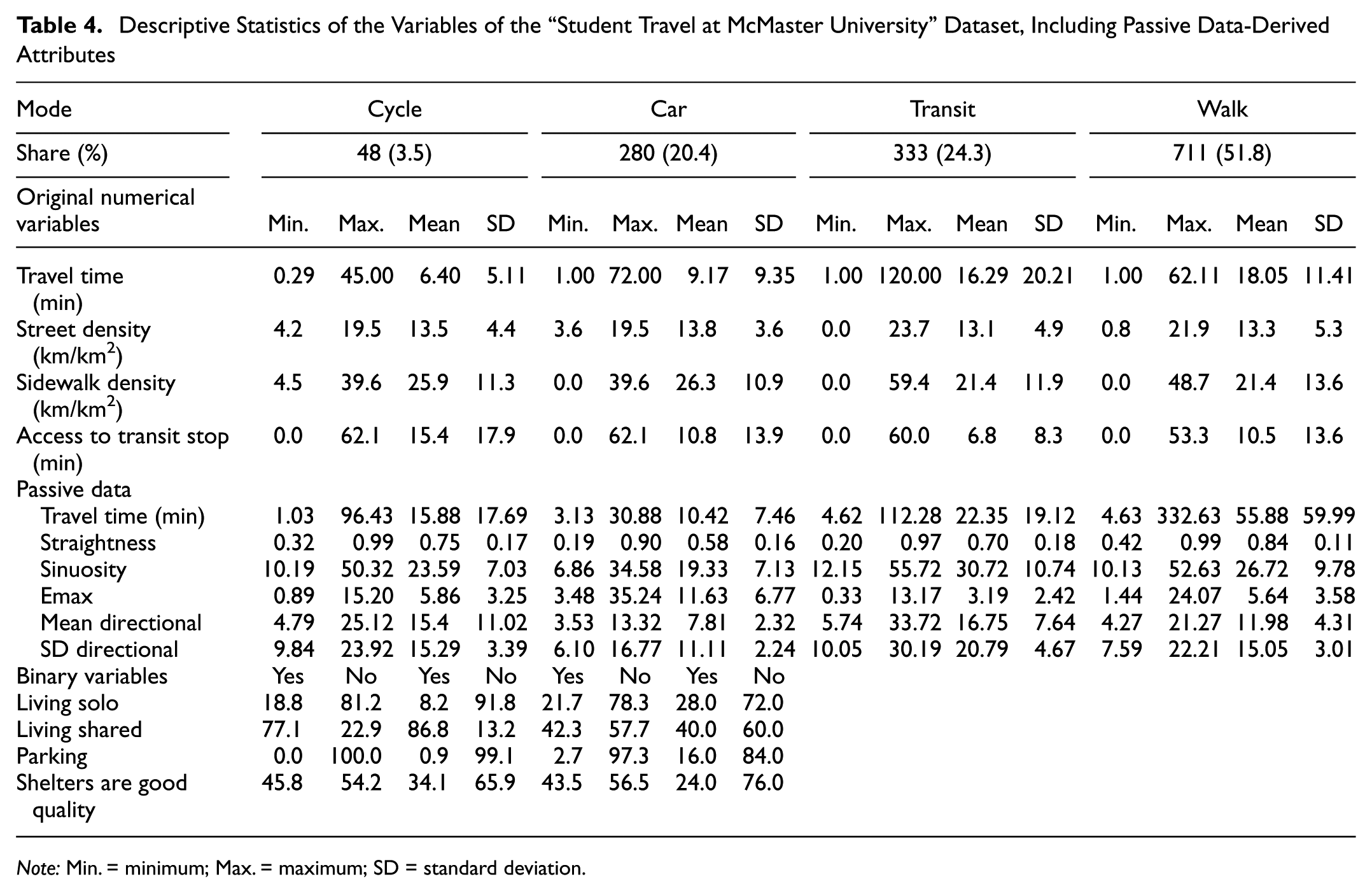
Note: Min. = minimum; Max. = maximum; SD = standard deviation.

Figure 2.

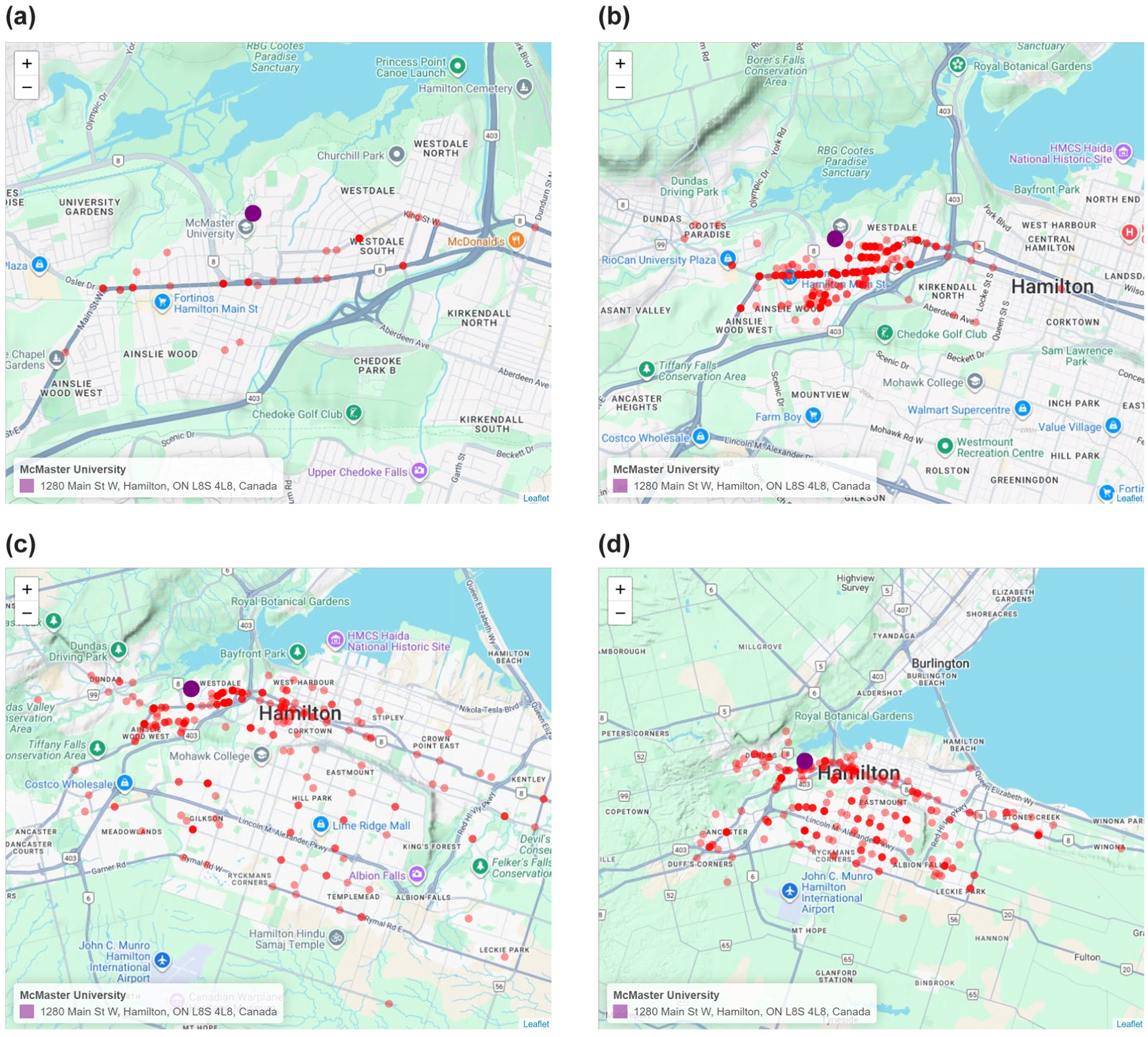
Geographical distribution of respondents by travel mode: (a) cycle, (b) walk, (c) transit, and (d) car.

Features Construction

To move beyond purely self-reported information, each OD pair was queried via the Google Maps API. For every respondent and for every available mode, we retrieved door-to-door travel time under prevailing conditions and the full polyline of the suggested route. From those polylines, we computed route-level geometric indicators that characterized the shape of each route. The complete set of predictors distinguishing RP data from passive sources is defined in Table 3, and descriptive statistics for the chosen mode are reported in Table 4.

According to metrics presented in Table 4, the comparison between self-reported times and API times showed systematic gaps across all modes. For walk, the mean increased from 18.05 to 55.88 min; for cycle, from 6.40 to 15.88 min; for bus, from 16.29 to 22.35 min; and for car, from 9.17 to 10.42 min. A diagnostic analysis of walking travel times revealed substantial dispersion in API-derived estimates, including a small number of extreme values. Manual inspection of these cases showed that they corresponded to OD pairs located at the periphery of the study area, where pedestrian routing involves indirect paths owing to network discontinuities, restricted crossings, or major road infrastructure. In contrast, self-reported walking times likely reflected perceived travel effort rather than strictly network-constrained routes. No unit-conversion errors or failed API queries were identified.

Passive route geometry exhibited clear, mode-consistent patterns. average straightness was highest for walk ( $0.84$ ) and cycle ( $0.75$ ), intermediate for bus ( $0.70$ ), and lowest for car ( $0.58$ ), whereas sinuosity followed the inverse ordering (bus: $30.72$ , walk: $26.72$ , cycle: $23.59$ , car: $19.33$ ). The maximum deviation, $E_{\max}$ , was largest for car (mean $= 11.63$ ), consistent with greater detours relative to the straight OD line, and smaller for bus ( $3.19$ ), walk ( $5.64$ ), and cycle ( $5.86$ ). Directional-change statistics reinforced these differences: the bus alternative showed the highest mean turning ( $16.75$ ) and variability (SD $= 20.79$ ), car the lowest (mean $= 7.81$ , SD $= 11.11$ ), with walk (mean $= 11.98$ , SD $= 15.05$ ) and cycle (mean $= 15.40$ , SD $= 15.29$ ) in between.

Survey context aligned with expected behavioral differences. Access time to the nearest transit stop was lowest for bus users (mean $= 6.8$ min) and higher for walk ( $10.5$ ), car ( $10.8$ ), and cycle ( $15.4$ ),suggesting that habitual bus riders live closer to transit. Street-density and sidewalk-density levels were of similar magnitude across modes, with a slightly higher average sidewalk density among cycle and car users. Campus parking permits were rare overall, with the highest incidence among walk (16.0%) and very low for car $/$ bus $/$ cycle ( $0.9 % to 2.7 %$ ). Housing arrangements also differed: the share living solo was largest for walk (28.0%) and bus (21.7%), whereas shared accommodation exceeded 75% among cycle and car respondents.

Taken together, Table 4 shows that passive attributes contributed information that was both systematic and complementary to RP measures. API travel times revealed underreporting in self-stated durations, and geometry-based variables captured network directness and detours that were unobservable in standard surveys, motivating their inclusion in the modeling scenarios that follow.

Modeling Scenarios

The objective of the modeling exercise was to assess how planner-derived variables—namely route-level geometric descriptors and planner-based travel times—affect predictive performance and interpretation relative to models relying solely on survey information. Travel mode choice was formulated as a four-class classification problem (walk, transit, car, cycle), and we estimated a set of tree-based classifiers, including CART, RF, XGBoost, and AdaBoost. These models are well suited to capturing the nonlinearities and interaction effects commonly observed in travel behavior data.

The dataset was split once into a training set (80%) and a held-out test set (20%) using stratified sampling by travel mode. All model development steps were strictly confined to the training data. Hyperparameters were tuned via Bayesian optimization combined with stratified repeated $K$ -fold cross-validation, with the objective of maximizing the macro-averaged $F_{1}$ -score, which ensures balanced evaluation across travel modes in the presence of class imbalance.

Rather than modifying the empirical class distribution through data resampling, class imbalance was addressed through cost-sensitive learning. Specifically, class weights inversely proportional to class frequencies were incorporated into the learning algorithms whenever supported. This strategy preserves the original data-generating process while penalizing misclassification of underrepresented modes during training. All preprocessing steps—including missing-value imputation, encoding, scaling, and class weighting—were embedded within a unified pipeline and applied only to the training portion of each cross-validation fold, ensuring a leakage-free evaluation.

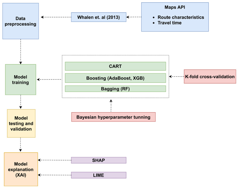
After identifying the optimal hyperparameter configuration, each model was retrained on the full training set using the same pipeline specification. Predictive performance was then evaluated once on the held-out test set using accuracy, precision, recall, and $F_{1}$ -score, reported in both per-class and in macro-averaged form. Figure 3 summarizes the complete modeling workflow, including preprocessing, class-weighted learning, hyperparameter tuning, refitting, and final evaluation.

Figure 3.

Modeling workflow.

To disentangle the contribution of different sources of information, we defined three modeling scenarios:

Scenario A (survey only): models trained using the original RP variables, including self-reported travel times, sociodemographic attributes, and contextual indicators.

Scenario B (survey + route geometry): models trained using the survey variables augmented with route-level geometric descriptors derived from the travel planner, such as straightness, maximum angular deviation, and directional variability, while retaining self-reported travel times.

Scenario C (survey + passive times): models trained using the full set of variables, combining survey data with both planner-derived travel times and route-level geometric descriptors.

Results

This section reports the predictive performance obtained in the three experimental settings. All metrics discussed below refer to the held-out test folds of the $5 \times 10$ stratified cross-validation. Each model was first tuned on the training portion (80% of the data) via the Bayesian optimization procedure using the values from Table 2; the resulting hyperparameters were then refitted on the whole training split and evaluated on the remaining 20%. Alongside the numerical scores we present SHAP and LIME visualizations to assess how the addition of API-derived travel times and route-geometry variables affected mode-choice explanations.

Optimal Hyperparameters

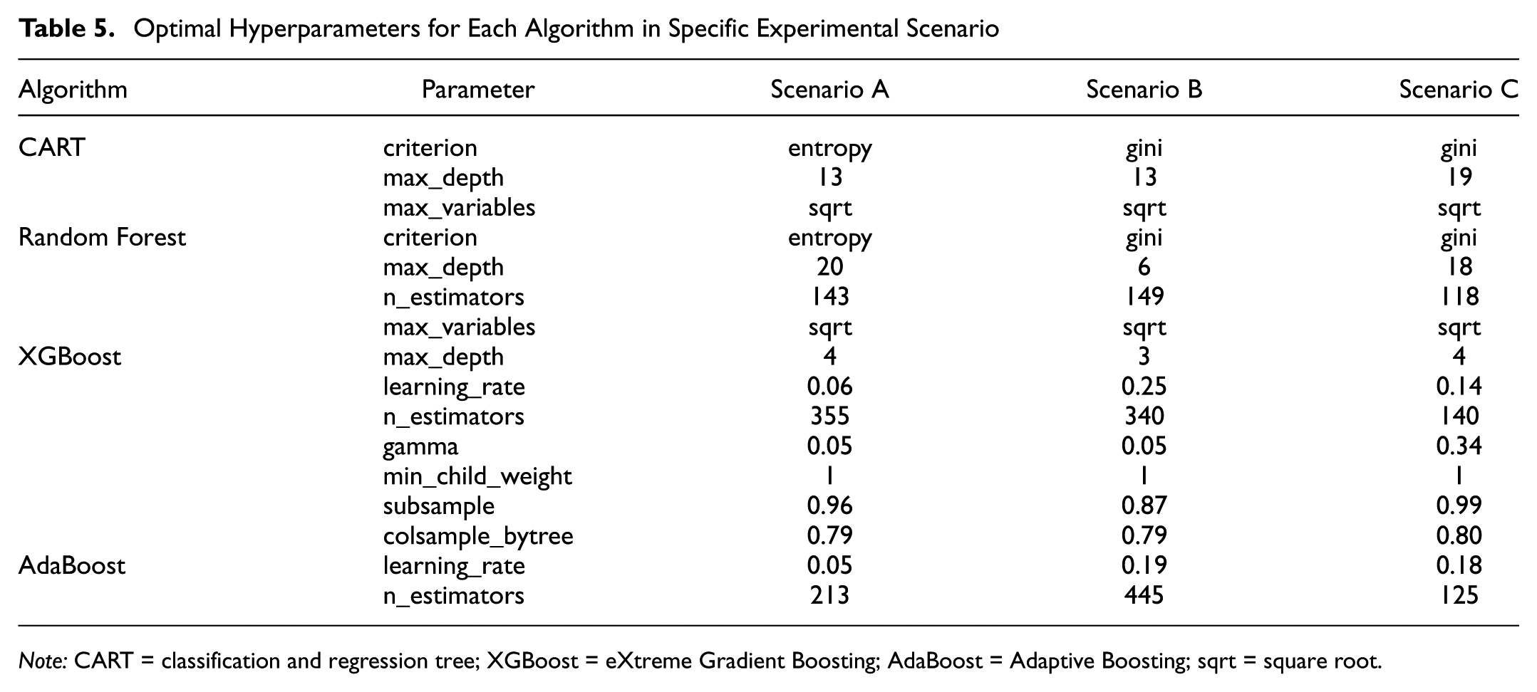
Table 5 reports the best hyperparameter settings selected by Bayesian optimization for each classifier and each of the three experimental settings. Each value corresponds to the configuration that maximized the mean macro- $F_{1}$ during the inner $5 \times 10$ stratified cross-validation; the same configuration was then refit on the full training split and evaluated on the test folds.

Table 5.

Optimal Hyperparameters for Each Algorithm in Specific Experimental Scenario

Algorithm	Parameter	Scenario A	Scenario B	Scenario C
CART	criterion	entropy	gini	gini
	max_depth	13	13	19
	max_variables	sqrt	sqrt	sqrt
Random Forest	criterion	entropy	gini	gini
	max_depth	20	6	18
	n_estimators	143	149	118
	max_variables	sqrt	sqrt	sqrt
XGBoost	max_depth	4	3	4
	learning_rate	0.06	0.25	0.14
	n_estimators	355	340	140
	gamma	0.05	0.05	0.34
	min_child_weight	1	1	1
	subsample	0.96	0.87	0.99
	colsample_bytree	0.79	0.79	0.80
AdaBoost	learning_rate	0.05	0.19	0.18
AdaBoost	n_estimators	213	445	125

Note: CART = classification and regression tree; XGBoost = eXtreme Gradient Boosting; AdaBoost = Adaptive Boosting; sqrt = square root.

Predictive Performance Across Modeling Scenarios

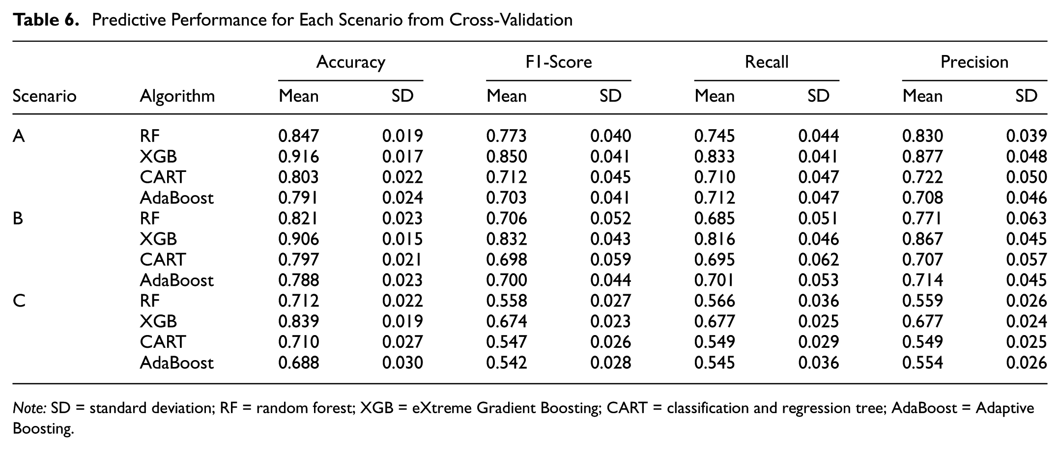
Table 6 reports the average predictive performance and associated variability obtained through repeated cross-validation across the three modeling scenarios. Across all settings, XGBoost consistently emerged as the best-performing algorithm, achieving the highest accuracy and macro-F1 values while exhibiting relatively low standard deviations. This indicates both strong predictive capability and robustness to variations in the training data.

Table 6.

Predictive Performance for Each Scenario from Cross-Validation

		Accuracy		F1-Score		Recall		Precision
Scenario	Algorithm	Mean	SD	Mean	SD	Mean	SD	Mean	SD
A	RF	0.847	0.019	0.773	0.040	0.745	0.044	0.830	0.039
	XGB	0.916	0.017	0.850	0.041	0.833	0.041	0.877	0.048
	CART	0.803	0.022	0.712	0.045	0.710	0.047	0.722	0.050
	AdaBoost	0.791	0.024	0.703	0.041	0.712	0.047	0.708	0.046
B	RF	0.821	0.023	0.706	0.052	0.685	0.051	0.771	0.063
	XGB	0.906	0.015	0.832	0.043	0.816	0.046	0.867	0.045
	CART	0.797	0.021	0.698	0.059	0.695	0.062	0.707	0.057
	AdaBoost	0.788	0.023	0.700	0.044	0.701	0.053	0.714	0.045
C	RF	0.712	0.022	0.558	0.027	0.566	0.036	0.559	0.026
	XGB	0.839	0.019	0.674	0.023	0.677	0.025	0.677	0.024
	CART	0.710	0.027	0.547	0.026	0.549	0.029	0.549	0.025
	AdaBoost	0.688	0.030	0.542	0.028	0.545	0.036	0.554	0.026

Note: SD = standard deviation; RF = random forest; XGB = eXtreme Gradient Boosting; CART = classification and regression tree; AdaBoost = Adaptive Boosting.

Under Scenario A (survey only), models trained exclusively on self-reported variables had already achieved high predictive performance. In particular, XGBoost attained an average macro-F1 of 0.85, substantially outperforming RF and the simpler CART and AdaBoost models. This result confirmed that the RP survey contained a strong signal for explaining travel mode choice in the studied context.

The results for Scenario B (survey + route geometry) revealed a noteworthy pattern. Although no substantial gains in overall accuracy or macro-F1 were observed relative to Scenario A, the performance of XGBoost remained virtually unchanged. This indicates that incorporating route-level geometric descriptors did not introduce noise or degrade predictive performance, even if it did not yield immediate improvements in global metrics. In other words, geometric features provide complementary information without compromising model stability.

In contrast, Scenario C (survey + passive times) showed a clear and consistent decline in predictive performance across all algorithms, as reflected in both accuracy and macro F1-scores. This deterioration was particularly pronounced for models other than XGBoost, suggesting that the direct inclusion of planner-derived travel times did not enhance—and may even have hindered—generalization under cross-validation. This finding is consistent with earlier methodological concerns about temporal misalignment between survey-reported trips and API queries, as well as the proxy nature of planner-based travel times.

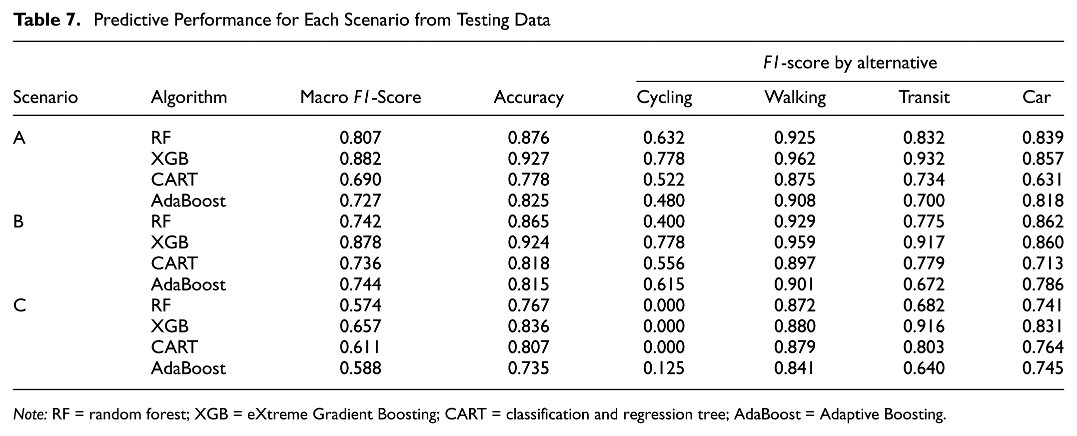
Table 7 presents predictive performance on the independent held-out test set, providing a direct assessment of out-of-sample generalization. The observed patterns reinforced the conclusions drawn from cross-validation.

Table 7.

Predictive Performance for Each Scenario from Testing Data

				F1-score by alternative
Scenario	Algorithm	Macro F1-Score	Accuracy	Cycling	Walking	Transit	Car
A	RF	0.807	0.876	0.632	0.925	0.832	0.839
	XGB	0.882	0.927	0.778	0.962	0.932	0.857
	CART	0.690	0.778	0.522	0.875	0.734	0.631
	AdaBoost	0.727	0.825	0.480	0.908	0.700	0.818
B	RF	0.742	0.865	0.400	0.929	0.775	0.862
	XGB	0.878	0.924	0.778	0.959	0.917	0.860
	CART	0.736	0.818	0.556	0.897	0.779	0.713
	AdaBoost	0.744	0.815	0.615	0.901	0.672	0.786
C	RF	0.574	0.767	0.000	0.872	0.682	0.741
	XGB	0.657	0.836	0.000	0.880	0.916	0.831
	CART	0.611	0.807	0.000	0.879	0.803	0.764
	AdaBoost	0.588	0.735	0.125	0.841	0.640	0.745

Note: RF = random forest; XGB = eXtreme Gradient Boosting; CART = classification and regression tree; AdaBoost = Adaptive Boosting.

In Scenario A, XGBoost achieved the strongest overall performance, with a macro-F1 of 0.882 and an accuracy of 0.927. The per-alternative analysis showed particularly strong performance for the walking, transit, and car modes, whereas cycling remained the most challenging alternative owing to its low prevalence, despite the use of cost-sensitive learning.

Scenario B yielded a key result for the contribution of the study. Although the macro-F1 achieved by XGBoost (0.878) was nearly identical to that of Scenario A, the per-class F1-scores indicated that the route-level geometric descriptors helped sustain—and in some cases reinforce—predictive performance for transit and car, without sacrificing accuracy for the remaining modes. This finding is particularly important, as it demonstrates that route geometry contains useful explanatory information for mode choice, even when it does not translate into higher aggregate performance metrics.

By contrast, Scenario C confirmed that incorporating API-derived travel times was not beneficial in this empirical setting. Macro-F1 values declined substantially, and the performance of the cycling alternative collapsed in several models, with F1-scores approaching zero. This behavior suggests that planner-derived travel times introduce inconsistencies that disproportionately affect minority classes, further supporting the methodological decision not to treat these estimates as direct counterfactuals of experienced travel time.

XAI Analysis: Comparative Insights from SHAP

Because XGBoost consistently achieved the highest macro- $F_{1}$ across experimental settings, the explainability analysis focused on this classifier to examine how the inclusion of passive data modifies the model’s decision logic. The objective was to assess both the global contribution of planner-derived attributes—travel times and route-level geometric descriptors—and their role in shaping mode-choice predictions across alternatives.

SHAP summary plots are used to visualize the distribution of SHAP values for each travel mode (Figure 4). Each point represents an individual trip, with its horizontal position indicating the SHAP value associated with a given variable, computed on the raw (pre-softmax) model outputs. Positive (negative) SHAP values increase (decrease) the relative competitiveness of a mode, and values farther from zero denote stronger influence. Color gradients indicate low-to-high feature values, enabling joint interpretation of effect direction and magnitude.

Figure 4.

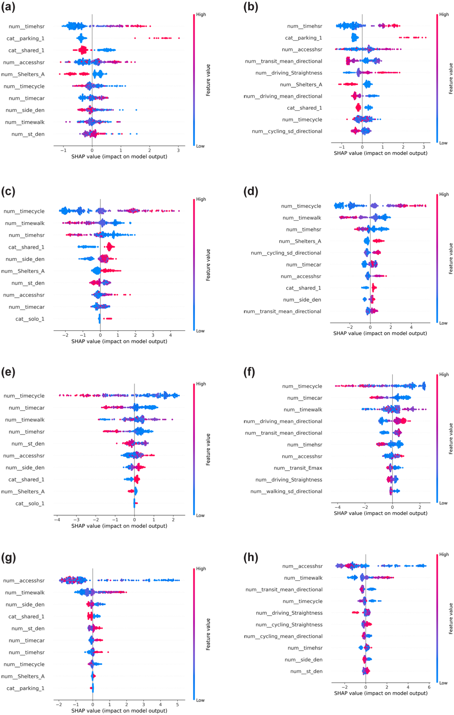
SHapley Additive exPlanations (SHAP) summary plots: (a) cycling—Scenario A, (b) cycling—Scenario B, (c) walking—Scenario A, (d) walking—Scenario B, (e) transit—Scenario A, (f) transit—Scenario B, (g) car—Scenario A, and (h) car—Scenario B.

The SHAP results revealed clear differences between the survey-only specification (Scenario A) and the augmented specification including planner-derived route attributes (Scenario B). Although predictive performance remained broadly comparable, the explanatory structure changed markedly once route-level information was introduced. In Scenario A, predictions were dominated by self-reported travel times and basic accessibility indicators, yielding relatively homogeneous explanations. In contrast, Scenario B exhibited a more diversified attribution structure, where route-geometry measures—such as straightness, maximum lateral deviation, and directional variability—emerged as systematic contributors, reflecting heterogeneous sensitivities to the network-constrained alternatives generated by the routing engine.

This effect is particularly pronounced for walking and cycling, for which route-geometry indicators ranked among the most influential predictors alongside travel time. For these active modes, less direct or more geometrically complex routes were generally associated with lower predicted choice probabilities, consistent with higher perceived travel effort or reduced route quality. For transit and car, geometric attributes played a secondary but consistent role, complementing traditional time- and access-based measures rather than replacing them. Importantly, these contributions reflected properties of standardized, planner-suggested routes rather than realized travel trajectories.

Overall, the SHAP analysis demonstrated that augmenting survey data with planner-derived route attributes did not necessarily lead to large gains in predictive accuracy, but it did substantially enrich the interpretability of the resulting models. By uncovering dimensions of route directness, complexity, and network structure that are not captured by self-reported variables alone, the augmented specification provided a more nuanced and transparent understanding of the factors underlying ML-based mode-choice predictions.

LIME: Local Explanations

To complement the global interpretability analysis provided by SHAP, we further examined local explanations using LIME. Whereas SHAP characterizes how features contribute on average across the sample, LIME offers instance-level explanations that clarify why a specific individual is assigned to a given travel mode. This local perspective is particularly relevant in transportation applications, in which policy interventions and planning decisions often target concrete travel situations rather than population averages.

Figure 5 presents LIME explanations for a randomly selected decision maker and predicted alternative (walk) under the survey-only specification (Scenario A) and the augmented specification with planner-derived attributes (Scenario B). The matched instances enable a direct comparison of how the model’s decision logic shifts when route-level information is incorporated.

Figure 5.

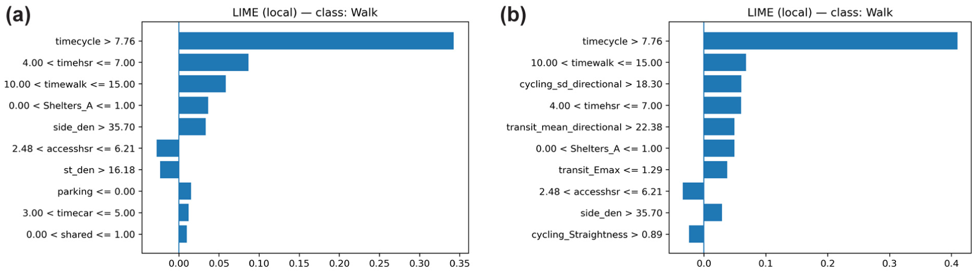
Local explanation from LIME for: (a) walk—Scenario A and (b) walk—Scenario B.

Under Scenario A, the local explanation was dominated by self-reported travel times, particularly cycling and walking times, with smaller contributions from basic accessibility and built-environment indicators. The explanation was relatively compact, reflecting a decision rule largely driven by perceived generalized cost. This mirrors the SHAP results for Scenario A, in which explanations were homogeneous and concentrated on a small subset of variables.

In contrast, the Scenario B explanation exhibited a richer and more nuanced structure. In addition to travel times, several planner-derived route descriptors—such as directional variability, cycling straightness, and maximum lateral deviation—entered the local explanation with nonnegligible contributions. These features modified the prediction by capturing aspects of route quality and complexity embedded in the network-constrained alternatives generated by the planner. Importantly, the inclusion of these attributes did not overturn the dominant role of travel time but refined the explanation by revealing how route geometry interacted with time-based measures for a specific individual.

Taken together, the LIME results reinforced the conclusions drawn from SHAP. Although the incorporation of planner-derived attributes did not systematically improve predictive performance, it substantially enhanced interpretability at both global and local levels. SHAP provided a stable overview of how route attributes reshaped the model’s attribution structure across modes, whereas LIME demonstrated how these same attributes translated into transparent, case-specific explanations. This complementarity supports the use of combined global–local explainability frameworks for ML-based travel behavior analysis, particularly when the goal is to inform interpretable and actionable transport planning decisions.

Consistency with Classical Discrete Choice Models

To complement the explainable machine-learning analysis, we estimated a Multinomial Logit (MNL) model (9) using the same augmented information set as in Scenario B. Estimation was carried out in the Apollo R package (67) using the Broyden–Fletcher–Goldfarb–Shanno (BFGS) algorithm. The purpose of this comparison is to assess behavioural consistency rather than predictive optimality.

The MNL estimates were largely consistent with the patterns identified by XGBoost and the SHAP/LIME analyses. Route-level geometric descriptors—such as straightness, maximum lateral deviation, and directional variability—entered the utility functions with statistically significant and theoretically coherent signs, indicating that more direct and geometrically simpler routes increased mode attractiveness. These effects aligned with the global SHAP results, where route geometry emerged as an important explanatory dimension, particularly for walking and transit. Self-reported travel time also remained a significant determinant, confirming its dominant behavioral role across modeling approaches.

In predictive terms, the MNL model exhibited substantially lower out-of-sample performance than XGBoost, with an overall accuracy of 0.57 and a macro $F_{1}$ -score of 0.31. This performance gap was expected given the restrictive structure of the MNL relative to flexible tree-based ensembles. Nevertheless, the MNL served as a transparent econometric benchmark that corroborated the behavioral plausibility of the ML explanations rather than competing on predictive accuracy.

Overall, the consistency between the MNL coefficients and the XAI results strengthened confidence in the substantive conclusions drawn from the ML analysis, indicating that planner-derived route attributes captured meaningful behavioral mechanisms rather than artifacts of the routing algorithm. Full estimation results and goodness-of-fit statistics for the MNL model are reported in Table A1.

Discussion and Conclusions

This study examined whether enriching RP survey data with planner-derived passive information improves travel mode-choice modeling in a general sense, using a university travel context as an illustrative application. The primary contribution lies not in the specific population analyzed, but in the proposal and validation of a transferable analytical pipeline that integrates survey data, route characterization from digital travel planners, ML algorithms, and XAI techniques within a unified framework.

From a predictive perspective, the results indicate that incorporating API-derived travel times does not systematically improve performance relative to models based on self-reported travel times. This suggests that self-reported measures already encode substantial behavioral content related to perception, experience, and adaptation to local travel conditions. Consequently, planner-based travel times offer limited marginal gains when such information is available, a finding that is likely to generalize beyond the empirical case considered here.

Importantly, the absence of systematic predictive improvements does not imply that passive data lack analytical value. When self-reported travel times are complemented with route-level geometric descriptors, models achieve comparable predictive performance while offering substantially richer interpretability. XAI analyses revealed that attributes describing route directness, geometric complexity, and directional variability contribute meaningfully to how alternatives are evaluated, uncovering behavioral mechanisms that remain hidden in survey-only specifications.

The joint use of SHAP and LIME underscores the complementary roles of global and local explanation in mode-choice analysis based on ML models. Whereas SHAP characterizes how the explanatory structure of the model changes when route-level information is introduced, LIME provides instance-level rationales that can be directly interpreted in planning terms. Together, these tools demonstrate that the main contribution of planner-derived route attributes lies in enhancing interpretability and behavioral insight rather than maximizing predictive accuracy.

To further contextualize these findings within the discrete choice modeling tradition, an MNL model was estimated using the same augmented information set. Although its predictive performance was substantially lower than that of tree-based ML models, the estimated coefficients exhibited signs and relative importance that were consistent with the XAI results. In particular, route-level geometric descriptors enter the utility functions in theoretically coherent ways, reinforcing the interpretation that these attributes capture meaningful behavioral dimensions rather than artifacts of the routing algorithm. This cross-paradigm consistency strengthens confidence in the substantive conclusions drawn from the ML analysis.

Methodologically, the proposed end-to-end pipeline represents a key contribution to data-driven travel behavior modeling. By linking RP surveys with standardized route characterization, flexible ML models, and transparent explanation techniques, the framework offers a reproducible approach for extracting actionable insight from enriched mobility data. This design is applicable to a wide range of travel mode-choice contexts, particularly in settings where large-scale passive mobility datasets are unavailable but routing services can provide consistent network-based proxies at low cost.

Future research should extend this framework by aligning planner-based queries with the exact timing of survey administration, enabling temporal consistency across congestion levels, service frequencies, and network conditions. Additional extensions include incorporating elevation, weather exposure, reliability, and crowding proxies, as well as applying the pipeline to different urban contexts and population groups. Finally, integrating predictive ML with causal inference methods represents a promising direction for moving from explanation toward policy evaluation.

Supplemental Material

sj-pdf-1-trr-10.1177_03611981261444331 – Supplemental material for Enhancing Travel Mode-Choice Modeling with Route-Based Attributes and Explainable Machine Learning

Supplemental material, sj-pdf-1-trr-10.1177_03611981261444331 for Enhancing Travel Mode-Choice Modeling with Route-Based Attributes and Explainable Machine Learning by Paticio Salas, Patricio Sáez and Lilian Barría in Transportation Research Record

Footnotes

Authors’ Note

GPT-4 assisted in editing the language.

Author Contributions

The authors confirm contribution to the paper as follows: study conception and design: P. Salas, P. Sáez, L. Barría; data collection: P. Salas, L. Barría; analysis and interpretation of results: P. Salas, P. Sáez, L. Barría; draft manuscript preparation: P. Salas, P. Sáez, L. Barría. All authors reviewed the results and approved the final version of the manuscript.

Declaration of Conflicting Interests

The authors declared no potential conflicts of interest with respect to the research, authorship, and/or publication of this article.

Funding

The authors disclosed receipt of the following financial support for the research, authorship, and/or publication of this article: This research was partially funded by ANID Fondecyt Iniciación 11250384 and ANID/CIN 250061.

ORCID iDs

Paticio Salas

Patricio Sáez

Supplemental Material

Supplemental material for this article is available online.

References

Hillel

Elshafie

M. Z. E. B.

Jin

Recreating Passenger Mode Choice-Sets for Transport Simulation: A Case Study of London, UK. Proceedings of the Institution of Civil Engineers - Smart Infrastructure and Construction, Vol. 171, No. 1, 2018, pp. 29–42.

Lunke

E. B.

Fearnley

Aarhaug

Public Transport Competitiveness vs. the Car: Impact of Relative Journey Time and Service Attributes. Research in Transportation Economics, Vol. 90, 2021b, pp. 1–8.

Tsoleridis

Choudhury

C. F.

Hess

Deriving Transport Appraisal Values from Emerging Revealed Preference Data. Transportation Research Part A: Policy and Practice, Vol. 165, 2022, pp. 225–245.

Cools

Deuse

Reiter

Biases in Self-Reported Travel Behaviour: Effects on Self-Reported Travel Distance, Travel Time and Rain Prevalence. Transportation Research Procedia, Vol. 76, 2024, pp. 62–69.

Houston

Luong

T. T.

Boarnet

M. G.

Tracking Daily Travel; Assessing Discrepancies between GPS-Derived and Self-Reported Travel Patterns. Transportation Research Part C: Emerging Technologies, Vol. 48, 2014, pp. 97–108.

Kelly

Krenn

Titze

Stopher

Foster

Quantifying the Difference between Self-Reported and Global Positioning Systems-Measured Journey Durations: A Systematic Review. Transport Reviews, Vol. 33, No. 4, 2013, pp. 443–459.

T. D.

Optimizing Urban Planning Through Spatial Network Analysis: A Case Study of Danang City. Geography, Environment, Sustainability, Vol. 18, No. 2, 2025, pp. 70–81.

Montello

D. R.

The Measurement of Cognitive Distance: Methods and Construct Validity. Journal of Environmental Psychology, Vol. 11, No. 2, 1991, pp. 101–122.

Benito-Moreno

Carpio-Pinedo

Lamíquiz-Daudén

P. J.

Proximity Features: A Random Forest Approach to the Influence of the Built Environment on Local Travel Behavior. Urban Science, Vol. 9, No. 4, 2025, p. 122.

10.

McFadden

Conditional Logit Analysis of Qualitative Choice Behavior, University of California, Berkeley, CA, 1972.

11.

Fafoutellis

Mantouka

E. G.

Vlahogianni

E. I.

Acceptance of a Pay-How-You-Drive Pricing Scheme for City Traffic: The Case of Athens. Transportation Research Part A: Policy and Practice, Vol. 156, 2022, pp. 270–284.

12.

Hagenauer

Helbich

A Comparative Study of Machine Learning Classifiers for Modeling Travel Mode Choice. Expert Systems with Applications, Vol. 78, 2017, pp. 273–282.

13.

Tang

Liu

Zhang

Exploring Urban Travel Patterns Using Density-Based Clustering with Multi-Attributes from Large-Scaled Vehicle Trajectories. Physica A: Statistical Mechanics and Its Applications, Vol. 561, 2021, pp. 1–15.

14.

Lundberg

S. M.

Lee

S.-I.

A Unified Approach to Interpreting Model Predictions. In Advances in Neural Information Processing Systems, Vol. 30, 2017, pp. 4765–4774.

15.

Ribeiro

M. T.

Singh

Guestrin

“Why Should I Trust You?”: Explaining the Predictions of Any Classifier, In KDD '16: Proceedings of the 22nd ACM SIGKDD International Conference on Knowledge Discovery and Data Mining, San Francisco, CA, August 13-17. 2016, pp. 1135–1144, ACM.

16.

Train

K. E.

Discrete Choice Methods with Simulation, 2009. Cambridge University Press.

17.

Gómez Mejía

Liberalización económica y crecimiento económico. Modelo Logit Multinomial aplicado a la metodología de” Doing Business”. Entramado, Vol. 7, No. 1, 2011, pp. 32–49.

18.

Sánchez

R. F. G.

Gaytán

M. P.

Análisis de la elección del consumidor entre tiendas de conveniencia y tiendas de abarrotes en Colima: Uso del modelo de regresión multinomial logit. Paradigma económico, Vol. 7, No. 2, 2015, pp. 27–46.

19.

Thrane

Examining Tourists’ Long-Distance Transportation Mode Choices Using a Multinomial Logit Regression Model. Tourism Management Perspectives, Vol. 15, 2015, pp. 115–121.

20.

Whalen

K. E.

Páez

Carrasco

J. A.

Mode Choice of University Students Commuting to School and the Role of Active Travel. Journal of Transport Geography, Vol. 31, 2013, pp. 132–142.

21.

Kalyanpad

N. G.

Hanni

C. K.

Rao

K. K.

Mode Choice Analysis Using Web-Based Revealed Preference Questionnaire, Stated Preference Experiment and Google Maps API. Transportation Research Procedia, Vol. 48, 2020, pp. 1–11.

22.

Lunke

E. B.

Fearnley

Aarhaug

Commute Trips in Norwegian Cities: Data Combining Trip Characteristics and Revealed Mode Choice. Data in Brief, Vol. 38, 2021a, p. 107319.

23.

Liu

Kelobonye

Zhou

Han

School Commuting Mode Shift: A Scenario Analysis for Active School Commuting Using GIS and Online Map API. International Journal of Geo-Information, Vol. 9, 2020, pp. 1–17.

24.

Lee

Unraveling the Impact of Travel Time, Cost, and Transit Burdens on Commute Mode Choice for Different Income and Age Groups. Transportation Research Part A: Policy and Practice, Vol. 141, 2020, pp. 147–166.

25.

Yang

En-Jian

Long

Nan

Taxi Route Choice Behavior Modeling Based on GPS Data. Journal of Transportation Systems Engineering and Information Technology, Vol. 15, No. 1, 2015, p. 81.

26.

Alwosheel

van Cranenburgh

Chorus

C. G.

Is Your Dataset Big Enough? Sample Size Requirements When Using Artificial Neural Networks for Discrete Choice Analysis. Journal of Choice Modelling, Vol. 28, 2018, pp. 167–182.

27.

Salas

De la Fuente

Astroza

Carrasco

J. A.

A Systematic Comparative Evaluation of Machine Learning Classifiers and Discrete Choice Models for Travel Mode Choice in the Presence of Response Heterogeneity. Expert Systems with Applications, Vol. 193, 2022, pp. 1–27.

28.

Ángel Martín-Baos

López-Gómez

J. A.

Rodriguez-Benitez

Hillel

García-Ródenas

A Prediction and Behavioural Analysis of Machine Learning Methods for Modelling Travel Mode Choice. Transportation Research Part C: Emerging Technologies, Vol. 156, 2023, pp. 1–35.

29.

Aziz

Youkee

N. K.

Ahmed

F. S.

Tasnim

Fahim-Ul-Islam

Chakrabarty

Enhancing Transparency in Transport Mode Detection: An Interpretable Ensemble Model Classifier. In 2024 International Conference on Advances in Computing, Communication, Electrical, and Smart Systems (iCACCESS), 2024, pp. 1–6. IEEE.

30.

Zhu

Zhang

Tan

Ran

Coupled Application of Generative Adversarial Networks and Conventional Neural Networks for Travel Mode Detection Using GPS Data. Transportation Research Part A: Policy and Practice, Vol. 136, 2020, pp. 282–292.

31.

Leveraging Explainable Artificial Intelligence and Big Trip Data to Understand Factors Influencing Willingness to Ridesharing. Travel Behaviour and Society, Vol. 31, 2023, pp. 284–294.

32.

Ngeni

Kutela

Chengula

T. J.

Ruseruka

Musau

Novat

Indah

D. A.

Kasomi

Prediction of Bike-Sharing Station Demand Using Explainable Artificial Intelligence. Machine Learning with Applications, Vol. 17, 2024, pp. 1–9.

33.

Sarker

M. A. A.

Asgari

Chowdhury

A. Z.

Jin

Exploring Micromobility Choice Behavior across Different Mode Users Using Machine Learning Methods. Multimodal Transportation, Vol. 3, No. 4, 2024, pp. 1–19.

34.

Kashifi

M. T.

Investigating Two-Wheelers Risk Factors for Severe Crashes Using an Interpretable Machine Learning Approach and SHAP Analysis. IATSS Research, Vol. 47, No. 3, 2023, pp. 357–371.

35.

Kashifi

M. T.

Robust Spatiotemporal Crash Risk Prediction with Gated Recurrent Convolution Network and Interpretable Insights from Shapley Additive Explanations. Engineering Applications of Artificial Intelligence, Vol. 127, 2024, p. 107379.

36.

Martín-Baos

J. Á.

López-Gómez

J. A.

Rodriguez-Benitez

Hillel

García-Ródenas

A Prediction and Behavioural Analysis of Machine Learning Methods for Modelling Travel Mode Choice. Transportation Research Part C: Emerging Technologies, Vol. 156, 2023, p. 104318.

37.

Jahangiri

Rakha

H. A.

Applying Machine Learning Techniques to Transportation Mode Recognition Using Mobile Phone Sensor Data. IEEE Transactions on Intelligent Transportation Systems, Vol. 16, No. 5, 2015, pp. 2406–2417.

38.

Tang

Xiong

Zhang

Decision Tree Method for Modeling Travel Mode Switching in a Dynamic Behavioral Process. Transportation Planning and Technology, Vol. 38, No. 8, 2015, pp. 833–850.

39.

Sekhar

C. R.

Madhu

Mode Choice Analysis Using Random Forrest Decision Trees. Transportation Research Procedia, Vol. 17, 2016, pp. 644–652.

40.

Wang

Ross

C. L.

Machine Learning Travel Mode Choices: Comparing the Performance of an Extreme Gradient Boosting Model with a Multinomial Logit Model. Transportation Research Record, Vol. 2672, 2018, pp. 35–45. 0361198118773556.

41.

Lee

Derrible

Pereira

Comparison of Four Types of Artificial Neural Network and a Multinomial Logit Model for Travel Mode Choice Modeling. Transportation Research Record, Vol. 2672, No. 49, 2018, pp. 101–112.

42.

Cheng

Chen

De Vos

Lai

Witlox

Applying a Random Forest Method Approach to Model Travel Mode Choice Behavior. Travel Behaviour and Society, Vol. 14, 2019, pp. 1–10.

43.

Sifringer

Lurkin

Alahi

Enhancing Discrete Choice Models with Representation Learning. Transportation Research Part B: Methodological, Vol. 140, 2020, pp. 236–261.

44.

Zhao

Yan

Van Hentenryck

Prediction and Behavioral Analysis of Travel Mode Choice: A Comparison of Machine Learning and Logit Models. Travel Behaviour and Society, Vol. 20, 2020, pp. 22–35.

45.

Wong

Farooq

Reslogit: A Residual Neural Network Logit Model for Data-Driven Choice Modelling. Transportation Research Part C: Emerging Technologies, Vol. 126, 2021, p. 103050.

46.

Kim

E.-J.

Analysis of Travel Mode Choice in Seoul Using an Interpretable Machine Learning Approach. Journal of Advanced Transportation, Vol. 2021, 2021, pp. 1–13.

47.

Han

Pereira

F. C.

Ben-Akiva

Zegras

A Neural-Embedded Discrete Choice Model: Learning Taste Representation with Strengthened Interpretability. Transportation Research Part B: Methodological, Vol. 163, 2022, pp. 166–186.

48.

Kashifi

M. T.

Jamal

Kashefi

M. S.

Almoshaogeh

Rahmane

S. M.

Predicting the Travel Mode Choice with Interpretable Machine Learning Techniques: A Comparative Study. Travel Behaviour and Society, Vol. 29, 2022, pp. 279–296.

49.

Liu

Loa

Wang

Habib

K. N.

Theory-Driven or Data-Driven? Modelling Ride-Sourcing Mode Choices Using Integrated Choice and Latent Variable Model and Multi-Task Learning Deep Neural Networks. Journal of Choice Modelling, Vol. 48, 2023, p. 100431.

50.

Ren

Yang

Chen

Cheng

Yuan

Exploring Passengers’ Choice of Transfer City in Air-to-Rail Intermodal Travel Using an Interpretable Ensemble Machine Learning Approach. Transportation, Vol. 51, 2023, pp. 1–31.

51.

Xia

Chen

Zimmermann

A Random Effect Bayesian Neural Network (RE-BNN) for Travel Mode Choice Analysis Across Multiple Regions. Travel Behaviour and Society, Vol. 30, 2023, pp. 118–134.

52.

Díaz-Ramírez

Estrada-García

J. A.

Figueroa-Sayago

Predicting Transport Mode Choice Preferences in a University District with Decision Tree-Based Models. City and Environment Interactions, Vol. 20, 2023, pp. 1–15.

53.

Arkoudi

Krueger

Azevedo

C. L.

Pereira

F. C.

Combining Discrete Choice Models and Neural Networks Through Embeddings: Formulation, Interpretability and Performance. Transportation Research Part B: Methodological, Vol. 175, 2023, p. 102783.

54.

Yang

Cui

Lin

Exploring Non-Linear and Synergistic Effects of Green Spaces on Active Travel Using Crowdsourced Data and Interpretable Machine Learning. Travel Behaviour and Society, Vol. 34, 2024, pp. 1–13.

55.

Batschelet

Circular Statistics in Biology. Mathematics in Biology, Academic Press, New York, 1981.

56.

Kitamura

Imafuku

Behavioural Mimicry in Flight Path of Batesian Intraspecific Polymorphic Butterfly Papilio Polytes. Proceedings. Biological Sciences / The Royal Society, Vol. 282, 2015, p. 20150483.

57.

Kahle

Wickham

Kahle

M. D.

Package ‘ggmap’. Retrieved September, Vol. 5, 2019, pp. 1–71.

58.

McLean

D. J.

Skowron Volponi

M. A.

TRAJR: An r Package for Characterisation of Animal Trajectories. Ethology, Vol. 124, No. 6, 2018, pp. 440–448.

59.

Breiman

Friedman

Olshen

Stone

Classification and Regression Trees. Wadsworth Int. Group, Vol. 37, No. 15, 1984, pp. 237–251.

60.

Breiman

Random Forests. Machine Learning, Vol. 45, No. 1, 2001, pp. 5–32.

61.

Freund

Schapire

R. E.

A Decision-Theoretic Generalization of on-Line Learning and an Application to Boosting. Journal of Computer and System Sciences, Vol. 55, No. 1, 1997, pp. 119–139.

62.

Chen

Guestrin

Xgboost: A Scalable Tree Boosting System. In Proceedings of the 22nd ACM SIGKDD International Conference on Knowledge Discovery and Data Mining, 2016, Association for Computing Machinery, San Francisco, pp. 785–794.

63.

Breiman

Bagging Predictors. Machine Learning, Vol. 24, No. 2, 1996, pp. 123–140.

64.

Hastie

Tibshirani

Friedman

J. H.

Friedman

J. H.

The Elements of Statistical Learning: Data Mining, Inference, and Prediction, Springer Series in Statistics, New York, Vol. 2, 2009.

65.

Shapley

L. S.

A Value for n-Person Games. Contributions to the Theory of Games, Vol. 2, No. 28, 1953, pp. 307–317.

66.

Molnar

Interpretable Machine Learning, 2019. https://christophm.github.io/interpretable-ml-book/.

67.

Hess

Palma

Apollo: A Flexible, Powerful and Customisable Freeware Package for Choice Model Estimation and Application. Journal of Choice Modelling, Vol. 32, 2019, p. 100170.

Supplementary Material

Please find the following supplemental material available below.

For Open Access articles published under a Creative Commons License, all supplemental material carries the same license as the article it is associated with.

For non-Open Access articles published, all supplemental material carries a non-exclusive license, and permission requests for re-use of supplemental material or any part of supplemental material shall be sent directly to the copyright owner as specified in the copyright notice associated with the article.

0.13 MB