Novel Estimation Method and Interpretation of the Peak Hour Factor at Intersections

Abstract

This study presents a statistically grounded method for estimating the peak hour factor (PHF) at intersections, using classical optimization techniques. Unlike the traditional approach, which computes a single ratio from aggregated turning movement volumes, the proposed method explicitly accounts for the count variability across individual turning movements and over multiple days. It produces not only a point estimate but also a confidence interval, offering a more defensible basis for analysis. The method implementation is quite straightforward: the optimization method revealed that PHF is actually the slope of the zero-intercept regression line between the peak interval flow rate and peak hourly volumes, in addition to generating its upper and lower 95^th percentile estimates. This finding enables a simple spreadsheet application of the estimation method. Regardless of the data aggregation intervals studied in this paper (5, 10, and 15 min), the traditionally estimated PHF fell outside of the proposed method’s 95% confidence interval in many cases, indicating a statistically significant difference between the outcomes of the two methods. This could result in under- or over-estimation of the design demand volumes in some cases.

Keywords

peak hour factor intersection turning movement count data aggregation Highway Capacity Manual

Introduction and Background

The peak hour factor (PHF) has been an enduring fixture in the U.S. capacity manuals since it made its first appearance 60 years ago, in the 1965 Highway Capacity Manual (HCM) release ( 1 ). At that time, separate PHF recommendations were proposed for freeways and intersections. For freeways, the recommended peak period was 5 min, yielding a theoretical PHF range of 0.083 to 1.0, while for intersections, a 15 min peak was proposed, yielding a PHF range of 0.25 to 1.0. Interestingly, for signalized intersections, the 1965 HCM recommended separate PHF’s for each intersection approach. Since then, subsequent HCMs have opted to apply a single, intersection-wide PHF to estimate the peak 15 min demand flow rate, which is used for adjusting the demand volumes for capacity and quality of service analyses (2 –6). PHF is commonly calculated as the sum of the peak hour turning movement volumes divided by the corresponding sum of the peak 15 min interval hourly flow rates.

As intersection turning movement data acquisition methods have advanced, the need for the use of PHF has diminished. Most agencies currently collect intersection turning movement counts (TMCs) in 15 min intervals—if not shorter—simplifying the identification of both the peak hour (within a 15 min window) as well as the 15 min peak flow period. This is simply done by multiplying each peak 15 min count by four. However, when a user is analyzing a future scenario with projected annual average daily traffic or hourly demands, the need for using PHF arises again. This has prompted a slew of studies aimed at collecting and developing default values of PHF that are context-dependent (e.g., urban versus rural, signalized versus stop control). A sampling of some of these key studies is presented next.

Tarko and Perez explored the variability of PHF within the same intersection and across multiple intersections ( 7 ). They found that PHF varied significantly at the same intersection across multiple weekdays. Figure 1 shows PHF variation by approach and weekday (non-consecutive). For the northbound approach in the AM peak, PHF ranged from 0.74 to 0.97 depending on the day. In fact, the authors found that day-to-day PHF variability was the largest contributor to variability across multiple intersections. The authors propose the use of a multi-day average PHF value for analysis.

Figure 1.

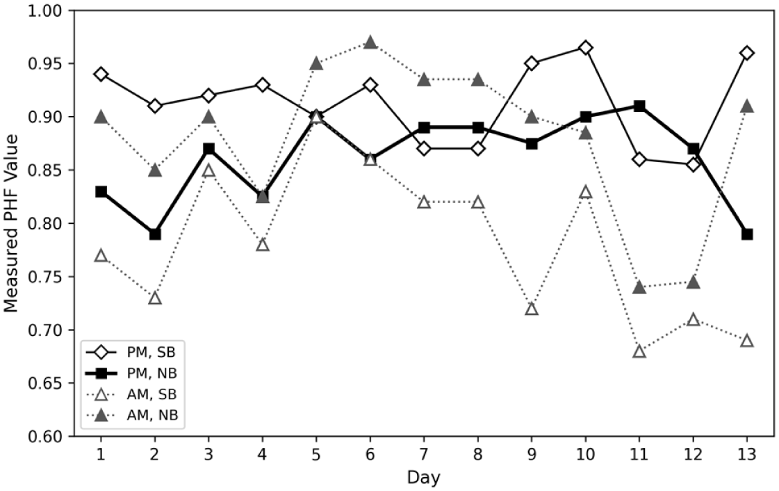
Peak hour factor day-to-day variation at a single site across multiple weekdays ( 7 ).

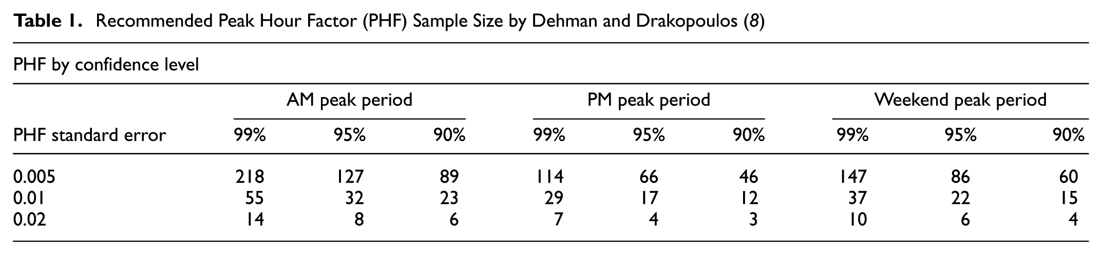
In a similar vein, Dehman and Drakopoulos collected a massive amount of PHF data (28,394 observations) in Milwaukee, WI, under different daily, seasonal, and operational conditions ( 8 ). One key recommendation they made was that the required sample size of PHF observations needed to characterize the true range of PHF.

Table 1 summarizes the required sample size observations based on time-of-day peak period, confidence level, and tolerable standard error (SE) of the mean value. For example, a user requiring the PHF estimator to be within 0.01 units from the true value 90% of the time in the PM peak period will need a sample size of 12 day observations at an intersection.

Table 1.

Recommended Peak Hour Factor (PHF) Sample Size by Dehman and Drakopoulos ( 8 )

PHF by confidence level
	AM peak period			PM peak period			Weekend peak period
PHF standard error	99%	95%	90%	99%	95%	90%	99%	95%	90%
0.005	218	127	89	114	66	46	147	86	60
0.01	55	32	23	29	17	12	37	22	15
0.02	14	8	6	7	4	3	10	6	4

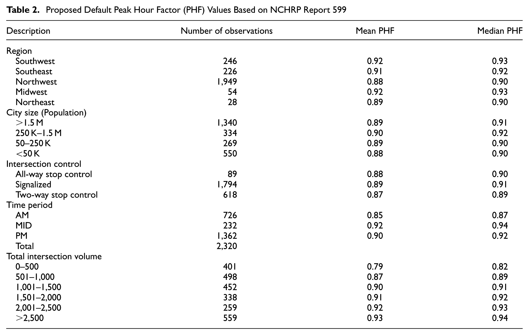
By far the most comprehensive study of PHFs is documented in NCHRP Report 599, which developed a series of PHF default values across multiple facilities using a nationwide data collection effort ( 9 ). Table 2 gives a summary of average and median PHF values by region, population, control, time-of-day peak period, and volumes. That study was the primary source of much of the PHF values found in most recent HCMs.

Table 2.

Proposed Default Peak Hour Factor (PHF) Values Based on NCHRP Report 599

Description	Number of observations	Mean PHF	Median PHF
Region
Southwest	246	0.92	0.93
Southeast	226	0.91	0.92
Northwest	1,949	0.88	0.90
Midwest	54	0.92	0.93
Northeast	28	0.89	0.90
City size (Population)
>1.5 M	1,340	0.89	0.91
250 K–1.5 M	334	0.90	0.92
50–250 K	269	0.89	0.90
<50 K	550	0.88	0.90
Intersection control
All-way stop control	89	0.88	0.90
Signalized	1,794	0.89	0.91
Two-way stop control	618	0.87	0.89
Time period
AM	726	0.85	0.87
MID	232	0.92	0.94
PM	1,362	0.90	0.92
Total	2,320
Total intersection volume
0–500	401	0.79	0.82
501–1,000	498	0.87	0.89
1,001–1,500	452	0.90	0.91
1,501–2,000	338	0.91	0.92
2,001–2,500	259	0.92	0.93
>2,500	559	0.93	0.94

A 2009 study by Yi et al. explored the distribution of a “peak flow factor” (PFF) as a generalization of the traditional PHF ( 10 ). They tested the stability of the PFF values under multiple aggregation periods varying from 3 to 15 min at six interrupted and uninterrupted flow facilities in Ohio. Similar to previous studies, the authors found that the PFF value increased as the aggregation period increased. In addition, its variability decreased with an increase in the aggregation period. They recommended the use of 10 or 15 min aggregation periods, both of which yielded similar values of PFF, with a preference for the 10 min period which enables a more refined tracking of the congestion onset time.

Finally, the latest HCM release recommends slightly different default PHF values for signalized and un-signalized intersections than NCHRP Report 599 ( 6 ). For signalized intersections, HCM7 recommends the use of a PHF default of 0.92 when the total entering volume equals or exceeds 1,000 vehicles per hour (vph), and 0.90 when the entering flow falls below 1,000 vph ( 6 ). For stop and yield-controlled intersections, a flat default PHF value of 0.92 is recommended.

In general, the literature shows that PHF is a highly variable parameter that is inconsistent in value even within the same intersection approach across multiple days. Studies have recommended that multiple (daily) samples of PHF are collected to enable a more robust estimation of its true value. The studies also generally indicate that the PHF value increases with intersection volume, is higher during the PM peak, increases as the aggregation period increases, and does not vary significantly by type of control.

On the other hand, the reviewed literature on PHF lacked any exploration of its statistical properties, nor has any study taken advantage of the inherent variability in the individual TMCs within the peak hour at an intersection to directly estimate the PHF 95^th percentile confidence interval.

This paper presents a novel statistical interpretation of PHF. This analysis enables users to quantify the effects of individual turning movements, day-to-day fluctuations, and the length of data aggregation period on both the trend and variability in PHF.

Study Objectives

The objectives of the study are twofold:

To develop a robust and statistically defensible approach to estimate PHF at intersections and its variation across movements, days, and aggregation intervals.

To test and contrast the proposed estimation method against the traditional estimation approach using data from multiple intersections and to analyze and report on the differences across movements, days, and intervals.

A Statistical Definition of the Peak Hour Factor (PHF)

An “intersection PHF” is defined as the ratio of the hourly, turning movement volume count to the highest flow rate observed over a shorter period (typically 15 min, as per HCM) within the same peak hour. At an intersection, we label the vector of (typically 12) turning volumes observed over the entire peak hour as Y and the peak hourly flow rate in the peak interval within the peak hour as X. Ideally, both Y and X would include multiple observation days, at the same location, as proposed in several studies cited in the literature.

By definition therefore:

PHF = \frac{Y}{X} = \frac{\sum_{NT} y_{it}}{\sum_{NT} x_{it}} = \frac{E (Y)}{E (X)}

(1)

where

Y = the sum of the individual turning movement flow rates i in the full hour on day t,

X = the sum of the individual turning movement flow rates i in the peak interval within the hour on day t,

N = the number of turning movements across the intersection,

T = the number of observation days, and

E(.) = the expected value or average.

For example, if one considers counts taken at a four-legged intersection, observed over 5 days, then N = 12 and T = 5, and the total number of observations would be 60. Thus, the index it pertains to a specific turning movement i, for example eastbound-left, on day t in both the vectors Y and X.

It is evident that the manner in which the current/traditional PHF calculation is done is not sensitive to the variations in the individual turning volumes in both vectors Y and X. The conventional method simply calculates their sums (or averages) and produces a quick estimate of PHF, as per Equation 1. That is the basic process by which PHF has been defined and estimated, since its first appearance in the 1965 U.S. HCM.

In reality, when dealing with multiple turning movement observations over multiple days, one can/should estimate PHF more formally, by determining its optimal value using classical optimization techniques. This can be done by taking advantage of the knowledge of the entire set of observations in both X and Y, rather than just their sums or averages, as described in the next section.

PHF Model Formulation

We formulate the PHF estimation problem by minimizing the estimation errors between the two vectors $\hat{Y}$ and Y. By definition, each hourly estimate of a turning movement i observation y_it on day t is defined as ${\hat{y}}_{it}$ = $PHF \times x_{it}$ yielding the error term ER for movement i as

E R_{i} = \sum_{T} (y_{it} - PHF \times x_{it}) .

The solution can now be formulated as an unconstrained minimization problem across all movements N and days T, as per Equation 2:

Minimize : ER = \sum_{N} \sum_{T} (y_{it} - PHF \times x_{it})^{2}

(2)

Decomposing the sums in Equation 2 yields:

ER = \sum y_{it}^{2} - 2 PHF \sum y_{it} x_{i} t + {PHF}^{2} \sum x_{it}^{2}

The minimum error solution occurs at $\frac{d (ER)}{d (PHF)} = 0$ , which yields:

- 2 \sum y_{it} x_{it} + 2 PHF \sum {x_{it}}^{2} = 0

Solving for PHF yields the formula:

PHF = \frac{\sum x_{it} y_{it}}{\sum x_{it}^{2}}

(3)

Using the method of expectations, Equation 3 can be rewritten as:

PHF = \frac{E (XY)}{E (X^{2})} = \frac{E (X) E (Y) + CO (X, Y)}{{[E (X)]}^{2} + VAR (X)}

(4)

Equation 4 gives the statistical properties of PHF. Of course, since the vector Y contains observations from X, vectors Y and X are not fully independent.

It is interesting to compare Equations 1 and 4. If one ignores both the variance and covariance terms in Equation 4, which one should not, the resulting PHF estimate would mirror that calculated from Equation 1.

Two special cases determine the boundary values of PHF. In the first case, X and Y vectors are assumed to be identical, that is, x_i = y_i for all values of i. Substituting those values in Equation 4 yields: PHF = $\frac{E (Y) E (Y) + COV (Y, Y)}{[E (Y)]^{2} + VAR (Y)}$ = 1.0

In the second case, a peak 15 min interval is considered. It assumes that all counts occur only during the peak 15 min peak. In this case, each x_i = 4 × y_i for all values of i. Substituting those values in Equation 4 yields:

PHF = \frac{E (4 Y) E (Y) + COV (4 Y, Y)}{{[E (4 Y)]}^{2} + VAR (4 Y)} = 0.25

Similarly, when a 5 min peak interval is considered, x_i = 12 y_i for all values of i and the corresponding PHF can be shown to be equal to 0.083.

Referring back to Equations 1 and 4, is it evident from Equation 4 that the parameter PHF is, in fact, identical to the slope of the zero-intercept regression model for the relationship:

Y = PHF \times X + ε

(5)

where

ε = an iid error term (see Hoel) ( 11 ).

The relationship in Equation 5 enables the analyst to utilize the entire vector of turning movements across multiple days, rather than just their sum or mean values.

The proposed PHF calibration approach not only produces estimates of its expected value but also ascertains the degree of model fit, the PHF variance across movements and days, and its 95^th percentile confidence interval for a given peak hour and across multiple days. Of interest to the users is how PHF, as estimated above, compares with the traditional approach exemplified by Equation 1, when analyzed over multiple days, and using different peak interval duration aggregation, for example 5, 10, and 15 min. This analysis is presented in this paper using empirical count data at several intersections, as described in the following sections. But first, some additional insights derived from Equation 4 above are presented.

Effect of Turning Movement Volume Variations

Equation 4 varies from the traditional approach by accounting for the variation in both the X and Y vectors in their variance and covariance, respectively. Using data from one of the test sites cited later in the paper, the effect of the disparity in turning movement volumes on the X and Y vectors was tested, and its effect on the estimated PHF analyzed. Table 3 shows 15 min TMCs taken at the intersection of Avent Ferry Road and Varsity Drive in Raleigh, North Carolina, during the PM peak hour. Also shown are the two vectors X and Y used to calculate PHF in the proposed method (i.e., Equation 4). Three scenarios are tested that compare the traditional and proposed estimation methods. In all three, the traditional PHF does not change, as long as the sums (or averages) of the X and Y vectors are unchanged. That PHF was calculated and equals 0.93.

Table 3.

PM Peak Hour Turning Movement Counts at Avent Ferry Road (AF) and Varsity Drive (VD)

Time	EB L VD	EB T VD	EB R VD	WB L VD	WB T VD	WB R VD	NB L AF	NB T AF	NB R AF	SB L AF	SB T AF	SB R AF
16:45	7	25	16	8	95	11	13	158	41	63	143	6
17:00*	16	37	29	6	114	20	13	159	43	64	159	12
17:15	14	25	17	5	96	15	16	142	43	76	168	19
17:30	14	37	31	5	69	14	19	134	30	61	172	10
Y vector	51	124	93	24	374	60	61	593	157	264	642	47
X vector	64	148	116	24	456	80	52	636	172	256	636	48

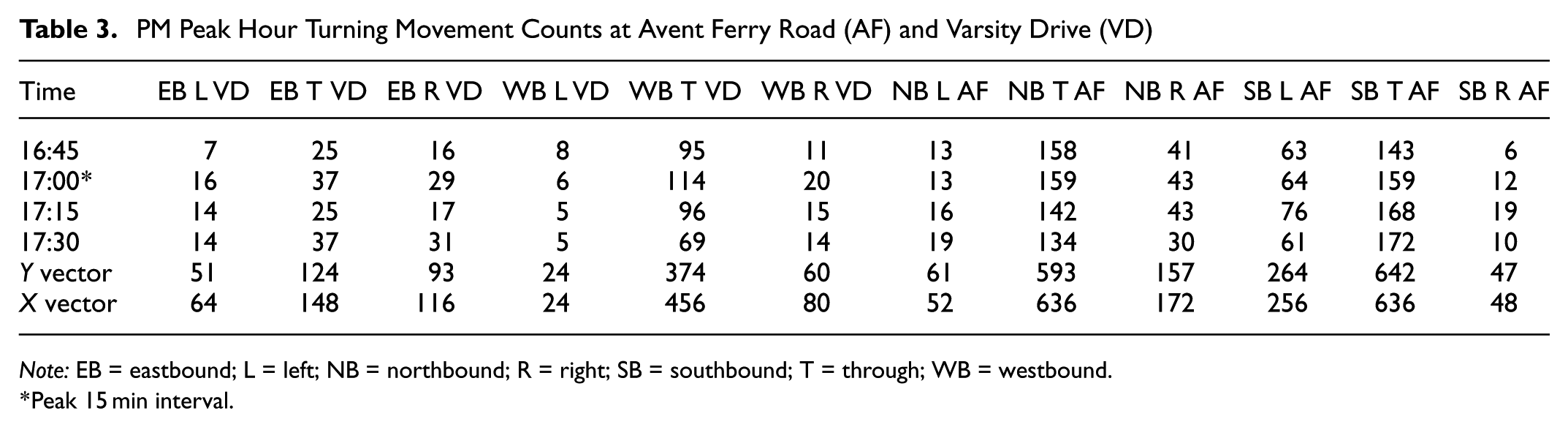
Note: EB = eastbound; L = left; NB = northbound; R = right; SB = southbound; T = through; WB = westbound.

*Peak 15 min interval.

The first scenario uses the existing TMCs to calculate the proposed PHF and its 95^th percentile confidence interval. In the second scenario, all left- and right-turning movements are zeroed out, and their counts added to the through-only count. This case essentially tests the effect of increasing the variance in the peak interval counts (only) on the resulting PHF. The last scenario does the opposite; it takes the overall intersection flow rate in the peak interval and distributes it equally to all turning movements. This emulates the case where no count variability occurs during the peak interval. The results from the three scenarios are summarized in Table 4, and discussed next.

Table 4.

Scenario Sensitivity Results at Avent Ferry Road and Varsity Drive

Scenario	E (X)	E (Y)	VAR (X)	COV (X, Y)	Proposed PHF	Lower 95th CI	Upper 95th CI	Traditional PHF estimate
1	158	147	46,076	43,680	0.94	0.89	0.99	0.93
2	158	147	101,132	69,848	0.74	0.62	0.86	0.93
3	158	147	0	0	0.93	0.44	1.41	0.93

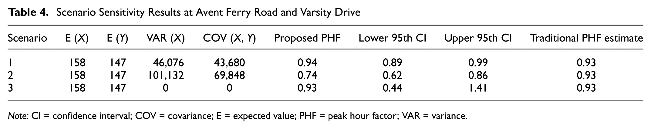
Note: CI = confidence interval; COV = covariance; E = expected value; PHF = peak hour factor; VAR = variance.

In Scenario 1, the proposed and traditional estimates are quite close (0.94 versus 0.93). Should an analyst decide to use a conservative estimate, the lower 95^th percentile value of PHF = 0.89 can be applied, denoting a steeper peaking profile. Scenario 2 essentially overloads the through traffic at the expense of zeroing out all left- and right-turning traffic. It results in higher values of both variance and covariance, and a steep reduction in the estimated PHF. In essence, the variability in X increased by 120% while the XY covariance increased by only 60%. This raises an interesting question, namely the conditions under which through traffic counts significantly exceed other turning movements. This is likely to occur at an intersection of a major arterial with a secondary or local road; the reverse pattern may occur on the secondary road where left- and right-turning TMCs on the minor road could exceed their through traffic ( 12 ). Thus, the closer the functional classifications of the two intersecting streets, the closer the two PHF estimates will be, while a large disparity in the two streets functional class will likely yield a lower proposed PHF estimate than the traditional method. Finally, Scenario 3 confirms the original thesis that the traditional method essentially ignores any variability in TMCs during the peak interval within the peak hour.

Test Sites and Data Description

Three intersections were selected in this study to test the new estimation method. These are: 1) Western Boulevard & Gorman Street, 2) Western Boulevard & Avent Ferry Road, and 3) Avent Ferry Road & Varsity Drive in Raleigh, North Carolina. They are referred to as Site 1, Site 2, and Site 3, respectively, in the subsequent sections. These intersections are typical four-legged, signalized intersections located near the North Carolina State University campus.

TMC data were collected at these sites over approximately 75 h, beginning at noon on the first day. The data collection days were chosen to represent typical weekday traffic patterns. Digital traffic counts were extracted using video analytics and aggregated into 5 min intervals ( 13 ). Figure 2 presents a time-series plot of total entering traffic in 5 min intervals, color-coded by site.

Figure 2.

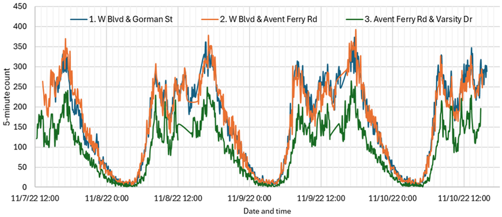
Time series plot of 5 min count data from three study intersections.

The data collection was nearly continuous, with minor interruptions between 12 noon and 3:30 p.m. because of battery replacements. Sites 1 and 2 experienced similarly high traffic volumes, primarily because Western Boulevard serves as a major arterial in Raleigh. The PM peak was more pronounced than the AM peak. Although midday traffic was also substantial, the peaking period was less well-defined than the AM and PM peaks. As a result, midday volumes were excluded from the peak hour analysis.

The data indicate that the AM and PM peaks were generally confined to a single hour. An exception was the AM peak on November 9, which extended beyond a 1 h window. Consequently, for each site, the peak hour was defined separately for the AM and PM periods as the single hour with the highest entering volume.

PHFs and Confidence Intervals

We estimated PHFs for each site separately for the AM and PM periods. Figure 3 illustrates a scatter plot of the peak hour volume (y-axis) versus the peak hourly flow rate (x-axis) for each site and peak period. Each plot includes 36 data points, representing 12 movements across 3 days. The straight line represents a zero-intercept linear regression model, with the slope corresponding to the proposed PHF as defined in Equation 4. A lack of data points is visible in the middle part of the plots, more so in the plots for the first two sites, which represents the difference in volume between the turning movements (shown on the left cluster) and higher-volume through movements (ones on the right). For Site 3, peak hour volume is more uniformly distributed across the movements.

Figure 3.

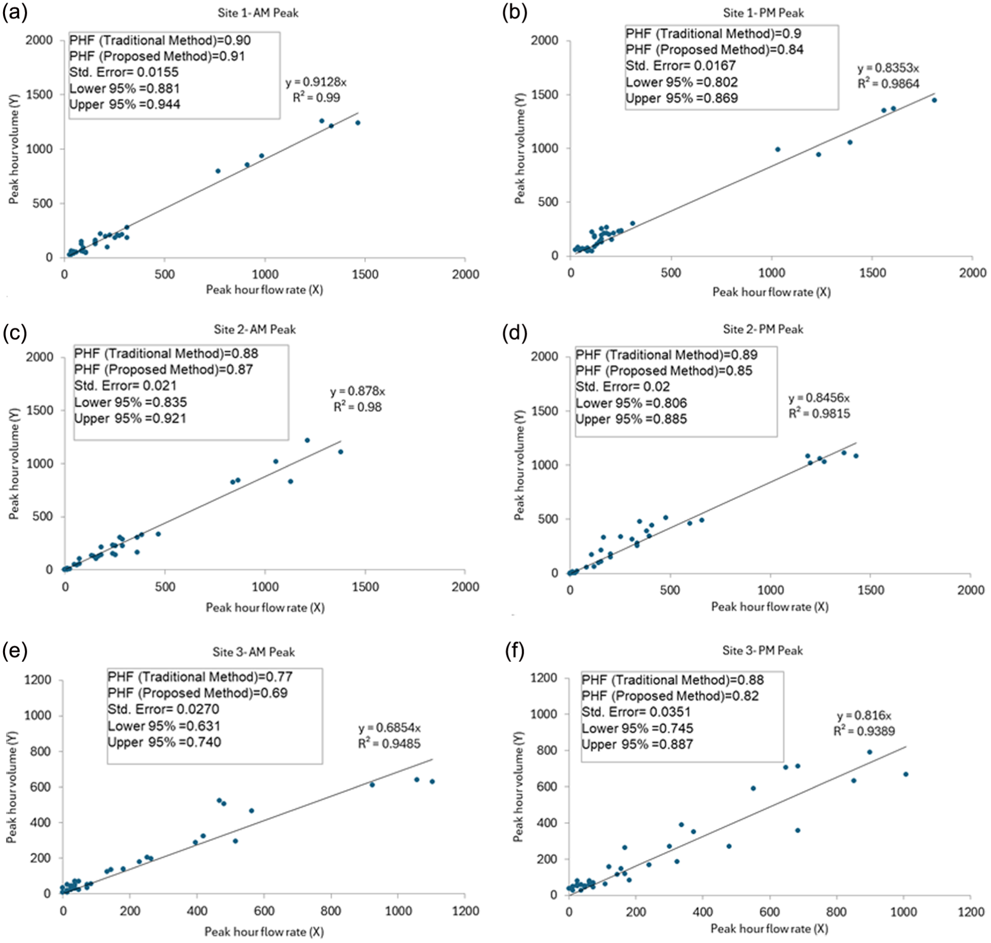
Peak hour factor (PHF) estimated from the peak hour volume and peak hour flow rate (using 5 min aggregated data over 3 days): (a) Site 1 AM peak, (b) Site 1 PM peak, (c) Site 2 AM peak, (d) Site 2 PM peak, (e) Site 3 AM peak, and (f) Site 3 PM peak.

The inset text box in each figure displays the PHF estimated using both the proposed method and the traditional method. For the proposed method, the PHF corresponds to the slope of the zero-intercept regression equation; its SE and the bounds of the 95% confidence interval are also shown. The SE is approximately 2%–4% of the estimated PHF, and the corresponding confidence interval spans roughly 0.07–0.14.

As shown in Figure 3, the PHF derived using the traditional method falls outside the 95% confidence interval of the proposed PHF in several cases (Figure 3, b , d , and e ), indicating a statistically significant difference between the estimates obtained from the two methods in these cases. The proposed method produces different PHF estimates because it accounts for the joint distribution of $X$ and $Y$ across multiple data points, whereas the traditional method relies on a single ratio calculation.

Figure 4, a and b , extends the comparison of PHF estimates of the two methods among the three sites using a different set of visuals. The PHFs estimated using the proposed method are shown with 95% confidence intervals, while traditional PHFs are plotted as red X markers.

Figure 4.

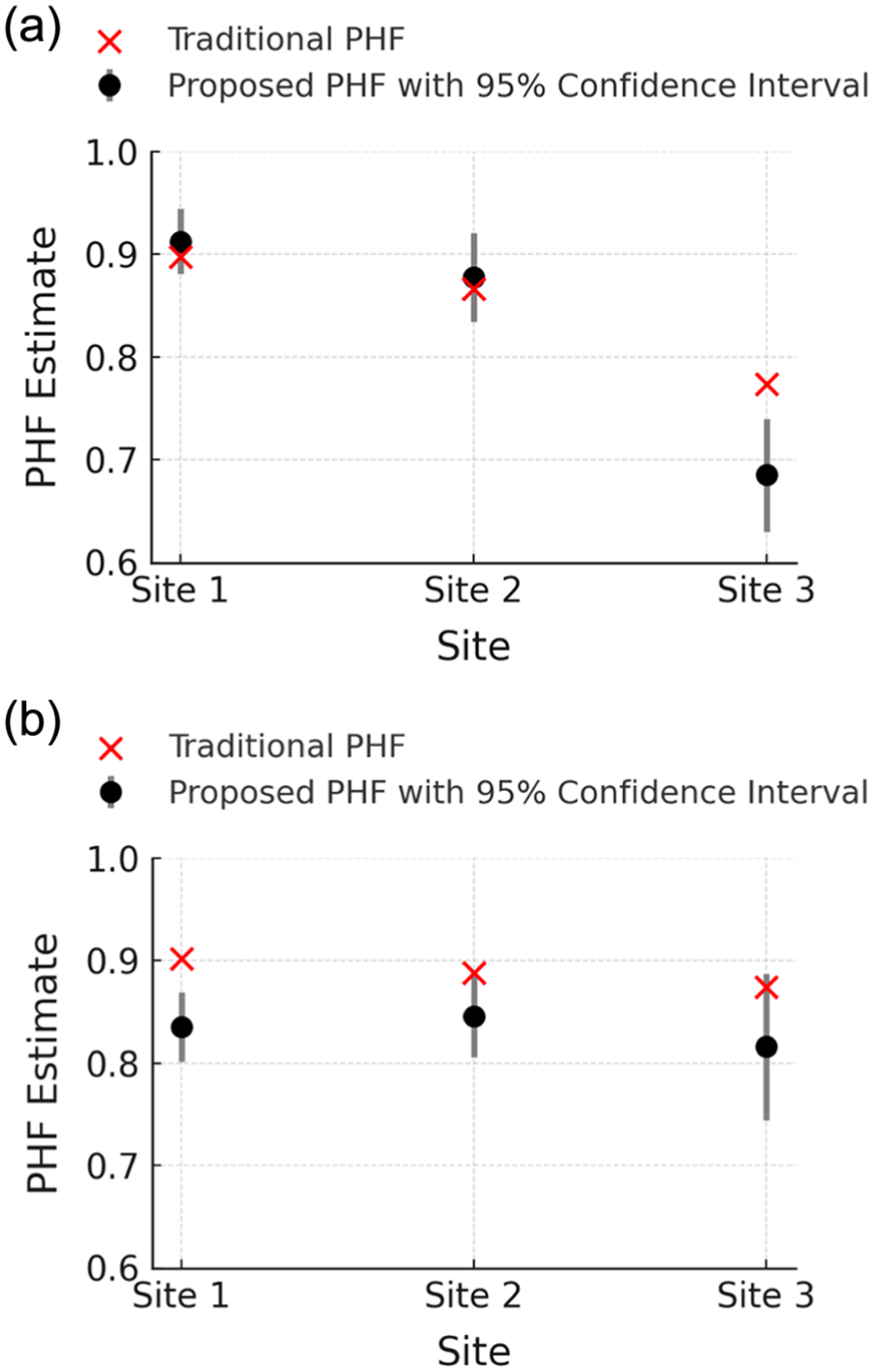
Peak hour factors (PHFs) with confidence intervals per the proposed method and traditionally estimated PHFs: (a) AM peak and (b) PM peak (using 5 min aggregated data).

The variation in PHF across sites is relatively consistent between the two methods. Site 3, which experiences the lowest traffic volume, also has the lowest PHF estimates in both AM and PM peak periods. This trend aligns with previous studies and guidance from HCM7, which suggest that lower-volume approaches typically yield lower PHFs because of a greater disparity between peak 15 min flow and total hourly volume ( 6 ). Site 3 also exhibits the widest confidence intervals—above 0.1, whereas for the other sites it hovers around 0.07—indicating greater variability in flow conditions.

While the proposed and traditional methods yield similar PHFs for Sites 1 and 2 during the AM peak, substantial differences emerge in the PM peak, especially for Site 3. In multiple cases, the traditional PHF exceeds the upper limit of the confidence interval around the proposed estimate, suggesting that it may underestimate the peak flow rate. However, as the subsequent sections will demonstrate, this is not universally true.

At this point, it is important to show that the traditionally estimated PHF often falls outside the 95% confidence interval of the proposed method’s estimates, even when using 10 and 15 min aggregated data. Since 15 min aggregation is the standard practice in traffic engineering, Table 5 focuses on this case, comparing traditional PHF values to the lower and upper bounds of the proposed method’s 95% confidence interval.

Table 5.

Traditionally Estimated Peak Hour Factor (PHF) and Confidence Intervals per the Proposed Method for 15 min Aggregated Data over 3 Days

Site ID	Traditional PHF	Proposed lower 95%	Proposed upper 95%
AM peak
Site 1	0.97	0.914	0.979
Site 2	0.95	0.962	1.038*
Site 3	0.95	0.818	0.881
PM peak
Site 1	0.96	0.952	0.985
Site 2	0.97	0.939	0.991
Site 3	0.93	0.900	0.995

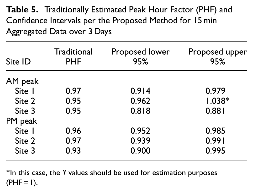
*In this case, the Y values should be used for estimation purposes (PHF = 1).

As expected, PHF estimates increase with coarser aggregation intervals—a trend that will be discussed in detail in a later section. Notably, in three out of six cases, the traditionally estimated PHF lies outside (or at the border of) the proposed method’s confidence interval, even though the interval itself becomes narrower (ranging from 0.03 to 0.10) compared with what was observed with 5 min data (which ranged from 0.06 to 0.14). This narrower range suggests reduced variability because of aggregation, but also underscores that, even at standard 15 min intervals, the traditional method can produce PHF values that significantly deviate from the statistically supported range.

Day-to-Day Variation of PHFs

Although previous studies have shown that traffic patterns can vary significantly from day to day at the same location and time, standard practice in traffic engineering often relies on data from a single “representative” day to estimate PHF ( 7 ). In this study, we also examined day-to-day variability by using traffic counts collected over multiple days. Table 6 presents PHFs estimated from individual days and to what extent they differ from the aggregated estimates across 3 days, using both the proposed and traditional methods.

Table 6.

Day-to-Day Variation of Peak Hour Factor (PHF) (Using 5 min Aggregated Data)

Site ID	Site name	Day	Proposed method	Traditional method
AM peak
Site 1	Western Boulevard & Gorman Street	AM day 2	0.93	0.90
		AM day 3	0.95	0.93
		AM day 4	0.87	0.86
		Max. PHF deviation (%) from combining 3 peaks	4%	4%
Site 2	Western Boulevard & Avent Ferry Road	AM day 2	0.92	0.87
		AM day 3	0.89	0.91
		AM day 4	0.84	0.82
		Max. PHF deviation (%) from combining 3 peaks	5%	6%
Site 3	Avent Ferry Road & Varsity Drive	AM day 2	0.64	0.72
		AM day 3	0.70	0.83
		AM day 4	0.72	0.77
		Max. PHF deviation (%) from combining 3 peaks	3%	8%
PM peak
Site 1	Western Boulevard & Gorman Street	PM day 1	0.84	0.93
		PM day 2	0.89	0.89
		PM day 3	0.79	0.89
		Max. PHF deviation (%) from combining 3 peaks	7%	3%
Site 2	Western Boulevard & Avent Ferry Road	PM day 1	0.85	0.89
		PM day 2	0.88	0.89
		PM day 3	0.81	0.88
		Max. PHF deviation (%) from combining 3 peaks	5%	1%
Site 3	Avent Ferry Road & Varsity Drive	PM day 1	0.79	0.87
		PM day 2	0.83	0.88
		PM day 3	0.82	0.87
		Max. PHF deviation (%) from combining 3 peaks	4%	1%

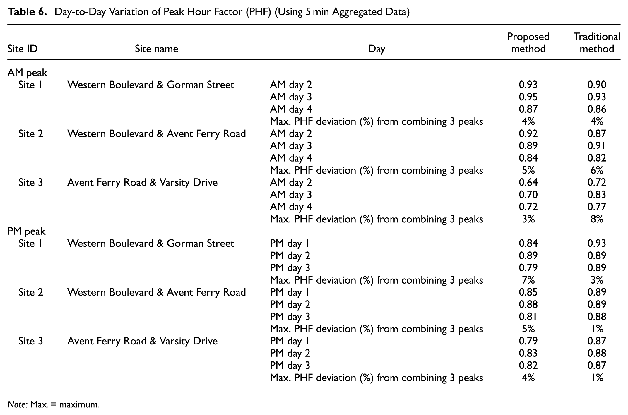
Note: Max. = maximum.

As shown in Table 6, PHFs derived from single-day data can differ by as much as 8% compared with those estimated from the combined 3 day dataset for the same intersection and peak period. During the AM peak, both methods generally reflect this day-to-day variation. In contrast, the traditionally estimated PHFs during the PM peak appear remarkably consistent across different days, possibly because of the method’s insensitivity to flow variability among different movements. The proposed method, on the other hand, accounts for the variation among different movements over multiple days which is reflected in the results.

While day-to-day deviations are not drastic in every case, relying on single-day counts can still result in meaningful over- or under-estimation of peak-hour traffic loads. It is important to note, however, that even using 3 days of data may not fully represent the long-term average or the “true” PHF. Additional data over extended periods would be necessary to assess the adequacy of multi-day sampling for PHF estimation.

Effects of Data Aggregation Interval

HCM7 pervasively uses 15 min aggregated data for all facilities. However, the use of finer aggregation intervals—such as 5 or 10 min data—is common when high-resolution data are available, as discussed in the literature review ( 10 ). While finer intervals can better capture short-term fluctuations in traffic flow, they may fail to represent steady-state operating conditions.

The aggregation interval is particularly relevant to this study, as the proposed method explicitly accounts for flow variability across movements and days—variability that tends to smooth out with coarser aggregation. Figure 5 presents PHF estimates across three aggregation intervals (5, 10, and 15 min), for both the proposed and traditional methods, during the AM and PM peak periods. The horizontal dashed line represents the HCM-recommended PHF (0.92) for signalized intersections with entering volumes exceeding 1,000 vph.

Figure 5.

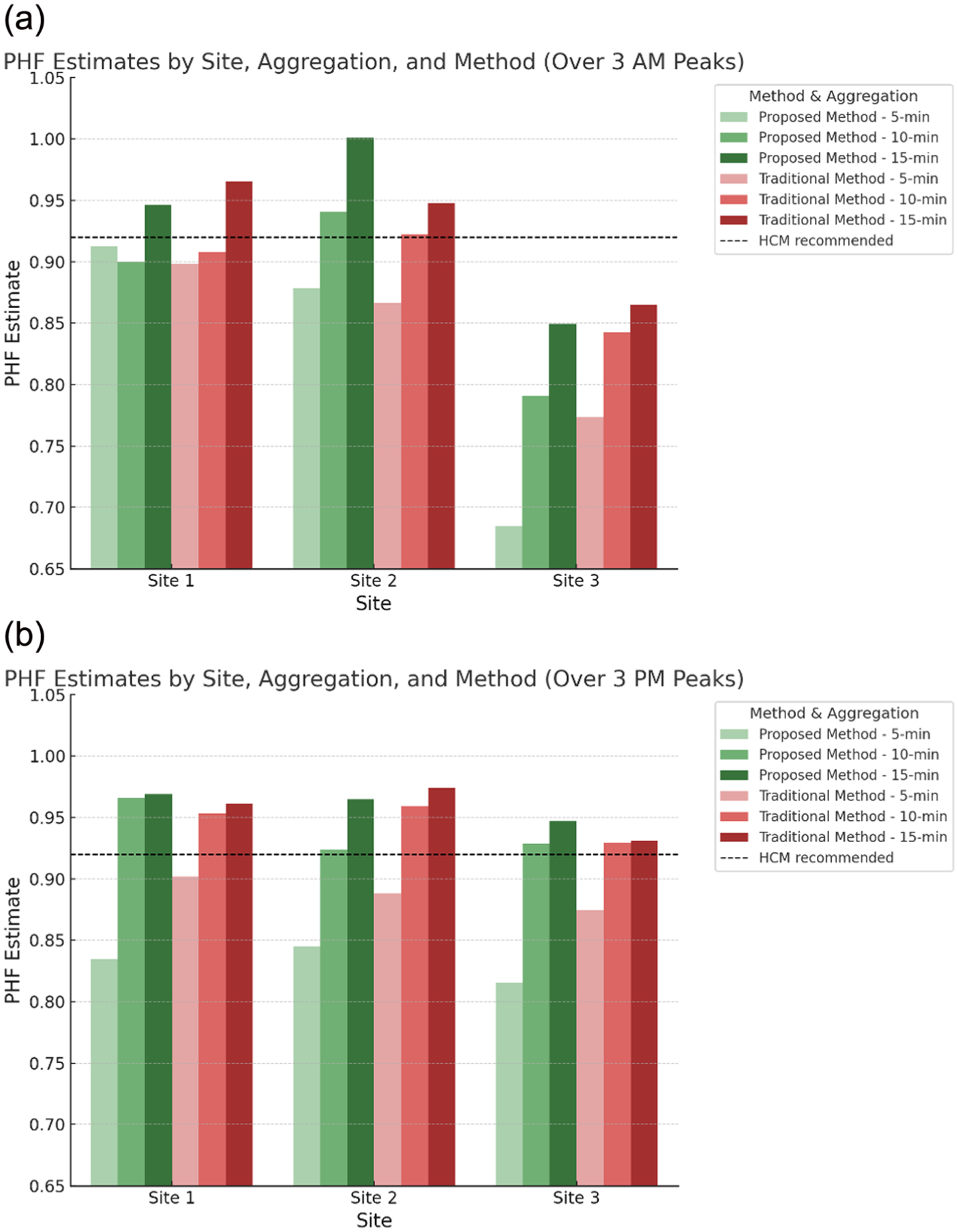
Peak hour factor (PHF) variation for different data aggregations and methods: (a) AM and (b) PM.

Key observations from Figure 5 are listed below:

Both methods are sensitive to the aggregation interval, with the proposed method generally showing greater sensitivity than the traditional method.

The most pronounced change in PHF occurs between the 5 and 10 min intervals. In contrast, the difference between 10 and 15 min estimates is relatively small, suggesting a diminishing effect beyond the 10 min threshold.

As expected, PHF increased with coarser data for almost all cases. The proposed PHF estimate for Site 1 AM peak is the only exception. It happened because the actual peak interval within the hour slightly shifted because of changing the aggregation interval, consequently changing the data used to calculate the PHF.

Aggregation effects vary by site and peak period studied. The PM peak exhibits stronger sensitivity to aggregation than the AM peak. Additionally, the effect is most prominent at Site 3, the lowest-volume intersection, where short-term spikes in flow excessively influence PHF estimates.

The choice of aggregation interval has policy implications. If a facility is intended to be designed for short-term peak flow (e.g., 5 min bursts), then using finer aggregation is justified. However, as shown in Figure 5, PHFs based on 5 min data—especially under the proposed method—are consistently lower than both the HCM-recommended value and typical PHFs used in signal design practice. This discrepancy is likely because of the lack of steady-state flow conditions at finer temporal resolutions, particularly at low-volume sites.

Conclusions and Recommendations

This study presented a statistically grounded method for estimating PHF at intersections. Unlike the traditional approach, which computes a single ratio from aggregate volumes, the proposed method explicitly accounts for variability across movements over days. It produces not only a point estimate but also a confidence interval, offering a more defensible basis for analysis. Regardless of the data aggregation interval, the traditionally estimated PHF was outside of the proposed method’s 95% confidence interval in many cases, indicating a statistically significant difference between the outcomes of the two methods. The 95% confidence interval was found to vary from 0.06 to 0.14 for 5 min and from 0.03 to 0.10 for 15 min aggregated data.

The results confirm that PHF is sensitive to both day-to-day variation and the aggregation interval used in data processing. The traditionally estimated PHF often appeared stable, especially during the PM peaks for the study sites, but this was largely because of its insensitivity to flow fluctuations. The proposed method, by contrast, revealed these variations, and aligned with prior findings by Dehman and Drakopoulos (8). In addition, larger differences between through-movements and TMCs at an intersection were associated with lower estimates of PHF based on the proposed method. This suggests that intersections of two roadways with widely different functional classes may yield lower PHF values. Testing this hypothesis is left for a future paper. Also included in any future research endeavor would be the influence of the proposed method of PHF estimation on key operational performance measures for intersections, for example, delay and queue length.

Aggregation intervals also played a key role. PHFs increased as the data were aggregated from 5 to 15 min intervals, with the largest change occurring between 5 and 10 min. The proposed method was more sensitive to this shift, particularly at low-volume sites. Notably, 5 min PHFs were often well below the HCM-recommended value.

The research proposed a statistical framework to estimate PHF and assess the accuracy by capturing variation across movements and time. Using field data, it also showed that practitioners should consider using multi-day data, especially at low-volume intersections. The agencies and the publishers of traffic operation guidebooks (e.g., HCM and the ITE Traffic Engineering Handbook) should introduce to the users the proposed method for estimating the confidence intervals of PHF. The available tools and software should incorporate the provision for entering multiple day counts and show the confidence intervals so that the practitioners can gauge the variation of traffic demand at an intersection.

Footnotes

Acknowledgements

This research was inspired as part of the TRB CIRCQS committee PHF Task Force. The authors are also thankful to the members of the Multimodal Connected Vehicle Pilot Evaluation Project for sharing the important data.

Author Contributions

The authors confirm contribution to the paper as follows: study conception and design: N. Rouphail; data collection: I. Ahmed; analysis and interpretation of results: N. Rouphail, I. Ahmed; draft manuscript preparation: N. Rouphail, I. Ahmed. All authors reviewed the results and approved the final version of the manuscript.

Declaration of Conflicting Interests

The authors declared no potential conflicts of interest with respect to the research, authorship, and/or publication of this article.

Funding

The authors received no financial support for the research, authorship, and/or publication of this article.

ORCID iDs

Nagui Rouphail

Ishtiak Ahmed

References

Transportation Research Board. Highway Capacity Manual. Special Report 87, Transportation Research Board, Washington, D.C., 1965.

Transportation Research Board. Highway Capacity Manual. Special Report 209, Transportation Research Board, Washington, D.C., 1985.

Transportation Research Board. Highway Capacity Manual. Transportation Research Board, Washington, D.C., 2000.

Transportation Research Board. Highway Capacity Manual. Transportation Research Board, Washington, D.C., 2010.

Transportation Research Board. Highway Capacity Manual. 6th edition: A Guide for Multimodal Mobility Analysis. Transportation Research Board, Washington, D.C., 2016.

Transportation Research Board. Highway Capacity Manual. 7th edition: A Guide for Multimodal Mobility Analysis. Transportation Research Board, Washington, D.C., 2022.

Tarko

Perez

Variability of a Peak Hour Factor at Intersections. Presented at the 84th Annual Meeting of the Transportation Research Board, Washington, D.C., January 9–13, 2005.

Dehman

Drakopoulos

Investigation of Peak-Hour Factor at Freeway Segments. Transportation Research Record: Journal of the Transportation Research Board, 2016. 2553: 117–127.

National Highway Cooperative Research Program Report 599. Default Values for Highway Capacity and Level of Service Analyses, Transportation Research Board, National Academy of Sciences, 2008, 125pp.

10.

P. J.

Wolfenbarger Raavi

V. S.

Investigation of Peak Flow Variations: Preliminary Field Studies. Transportation Research Record: Journal of the Transportation Research Board, 2009. 2130(1): 75–82. https://doi.org/10.3141/2130-10

11.

Hoel

Introduction to Mathematical Statistics Fourth Edition. John Wiley and Sons, Inc., New York.

12.

Iroanya

An Evaluation of Turning Movement Counts and Estimation of Initial Turning Movement Proportions. M.S. Thesis, Texas A&M University, December 2020, 81pp.

13.

STREET Simplified. Solving Crashes before they Happen. https://www.streetsimplified.com/. Accessed July 30, 2025.