Risk Assessment Method for Connected and Autonomous Vehicles Based on Traffic Factor Safety State Network and Risk Field Theory

Abstract

The driving risk of a vehicle is influenced not only by its own state, but also by the driving environment. With the development of smart connected technologies, vehicles can acquire more information about the environment. However, traditional driving risk assessment indicators only consider the impact of individual traffic factors and are unable to assess driving risk comprehensively. Moreover, they fail to evaluate the overall safety of mixed traffic flow from a macroscopic perspective. In this study, we model various types of risks based on the risk field theory and analyze the environmental impact factors of road sections based on the traffic factor safety state network theory, thereby proposing a microscopic vehicle risk field indicator VRFI and a novel macroscopic road risk field indicator RRFI. In the experiment part, we first verify the rationality of the microscopic vehicle risk assessment indicator VRFI through car-following and lane-changing scenarios, and then validate the effectiveness of the macroscopic road risk monitoring indicator RRFI using real-world traffic data and simulation techniques. Finally, we analyze the overall risk of traffic flow under different traffic states. This study provides an innovative method for microscopic risk assessment of connected and autonomous vehicles and macroscopic risk monitoring of mixed traffic flow.

Keywords

traffic factor safety state network risk field theory connected and autonomous vehicles driving risk assessment environmental impact factor

Introduction

The increasing number of vehicles on the road poses a significant challenge to driving safety. According to the World Health Organization, over 1.35 million fatalities and more than 50 million injuries occur annually as a result of road traffic accidents worldwide ( 1 ). As the automotive industry is moving toward intelligence and connectivity, smart connected technologies offer new opportunities to enhance road traffic safety, enabling connected and autonomous vehicles (CAVs) to obtain richer and more accurate environmental information ( 2 , 3 ). Therefore, how to fully utilize this perceived information to design more comprehensive and accurate driving risk assessment methods has become a research hotspot.

Driving safety risk assessment methods are usually divided into microscopic and macroscopic perspectives. Risk assessment from a macroscopic perspective relies on traffic flow data and crash data, which are used to evaluate the overall risk of a road or a specific area. These methods are commonly applied in traffic management departments. Yang et al. utilized high-resolution highway traffic data and constructed a risk assessment model by combining machine learning and statistical methods ( 4 ). The results demonstrate a significant correlation between traffic flow states and traffic safety. Zhao et al. constructed a convolutional neural network for forecasting crash risk across various traffic conditions ( 5 ). In addition, Xu et al. pointed out that different traffic states have different crash mechanisms, emphasizing the importance of traffic flow variables in assessing crash risk and developing a real-time crash risk model accordingly ( 6 ). However, these macroscopic risk assessment methods can only identify road risks under specific traffic states and are unable to achieve accurate quantitative assessment when facing complex and changing traffic states.

Microscopic risk assessment methods mainly rely on vehicle dynamics analysis, with research focusing on the safety threats faced by individual vehicles. This method characterizes the driving risk of vehicles by obtaining vehicle state information (such as speed and acceleration) and the relative motion relationships between two vehicles (such as relative speed and relative distance) (7 –9). It has been widely used in the study of car-following (10 –13) and lane-changing behavior ( 14 , 15 ). In practice, reasonable surrogate safety measures (SSMs) are often designed to quantify these risks ( 16 , 17 ), such as time-to-collision (TTC) and headway. However, the factors considered by these indicators are mostly only applicable to simple traffic scenarios. In the connected environment, vehicles can obtain richer traffic information, so it is necessary to optimize and improve the existing safety indicators to achieve more effective risk assessment.

With the advancement of sensor and connectivity technologies, an increasing number of risk assessment studies have begun to leverage real-time traffic data. Gore et al. developed a two-dimensional traffic conflict assessment framework based on the influence area of the subject vehicle, using variables such as traffic density, speed, and speed standard deviation, providing a feasible solution for real-time safety monitoring at the network level ( 18 ). Yuan et al. utilized traffic flow characteristics to develop real-time conflict prediction models, in which traffic volume and speed were identified as significant variables affecting traffic conflicts ( 19 , 20 ). Mogyorósi et al. employed a fuzzy logic approach to perform fuzzy-based risk classification for given road segments, capable of considering road curvature characteristics and weather impacts ( 21 ). However, these studies struggle to provide accurate quantitative assessments of overall road segment risk, focusing more on graded evaluations based on conflict frequency or general risk state differentiation.

Among traditional vehicle risk assessment metrics, (TTC), post-encroachment time (PET), and deceleration rate to avoid a crash (DRAC) are the most popular SSMs ( 22 ) and have been widely applied to safety issues such as vehicle-to-vehicle ( 23 ) and vehicle-to-pedestrian ( 24 ) collision risks. However, these metrics may not be fully suitable for CAVs. Do et al. investigated the applicability of conventional safety indicators to CAVs and found that TTC, DRAC, and PET are insufficient for measuring the safety impact of CAVs when consecutive vehicles travel at similar speeds ( 25 ). Recent studies have leveraged the rich data obtained through connectivity technologies to design more accurate risk assessment metrics for CAVs. Xu et al. employed reliability theory to develop a comprehensive potential safety risk assessment framework and an innovative SSM for capturing the potential safety risks of multiple preceding vehicles in car-following scenarios ( 26 ). Wang et al. proposed a novel probabilistic occupancy risk assessment metric that uses spatiotemporal heatmaps for probabilistic occupancy prediction of surrounding traffic participants and estimates collision risk along planned trajectories ( 27 ). Nevertheless, these methods are often limited to specific scenarios, cannot be easily extended to other complex situations, and fail to adequately reflect the influence of the overall road environment.

To achieve refined risk characterization, researchers have proposed the Artificial Potential Field theory, which was originally applied to robotic path planning and collision avoidance techniques ( 28 , 29 ). Subsequently, some scholars have extended this theory to the field of traffic research (30 –32). Wang et al. constructed the Driving Safety Field model, which integrates potential fields, kinetic energy fields, and behavioral fields (33 –35). Li et al. optimized the representation of distances between vehicles and improved the driving risk field model, establishing corresponding car-following and lane-changing models (36 –39).

However, the driving risk of CAVs should consider the impact of multiple factors, including the intelligence level of the vehicle itself and the influence of the road environment. Wang et al. defined the “road state factor” to express the specific impact of road states (such as the coefficient of adhesion, curvature, gradient, and visibility) on the driving risk field (33 –35). However, the definition of the “road state factor” is relatively idealized, its accuracy is difficult to verify, and there are difficulties in determining the relevant parameters. Cui et al. proposed the “operating environment complexity coefficient” to comprehensively consider the impact of road facilities, traffic flow, and climatic environment on driving risk ( 40 ). However, the calculation of this coefficient requires the road to be simply divided into four categories through the SRAAV (Road Safety Risk Assessment for Autonomous Vehicles) ( 41 ) method, and then the “operating environment complexity coefficient” is determined for each category of road, so it cannot accurately distinguish and refine the specific impact of different types of road environments. Therefore, how to reasonably determine the impact of different road environments on vehicle risk and comprehensively assess driving risk by combining environmental factors has become a key issue that urgently needs to be solved.

Many studies have highlighted that crash risk varies significantly across different traffic states, with strong correlations between traffic metrics (such as traffic volume and speed) and traffic safety states ( 42 ). For instance, Kwak and Kho utilized genetic programming techniques to develop crash risk models for both non-congested and congested conditions ( 43 ). Their findings indicated that changes in traffic state are associated with distinct traffic flow characteristics that contribute to crashes. In addition, Ding et al. established SSM thresholds using unsupervised learning to identify traffic conflicts under various traffic states ( 44 ). The study revealed that the distribution of traffic conflicts indeed varies across different traffic states. Therefore, distinguishing different traffic states by using real-time traffic flow metrics and then analyzing the impact of these states on driving risk can be a feasible way to measure the impact of the environment on driving risk.

Although existing models attempt to explain the interaction between traffic factors and the environment ( 45 , 46 ), understanding how these factors affect complex dynamic systems still faces certain challenges. Zhang et al. classified traffic factors into different categories and adopted a data-driven approach to use traffic data to mine the impact of these environmental factors (47 –51). This indicates that when complex traffic systems are difficult to model and analyze, using a data-driven approach can effectively reveal the impact of the road environment on traffic (52 –55).

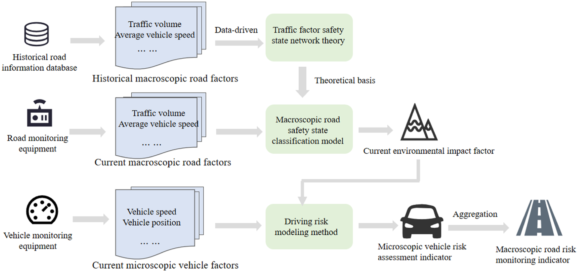
In light of the above discussion, this paper proposes a novel driving risk assessment method for CAVs based on the traffic factor safety state network (TFSSN) and the driving risk field theory. As shown in Figure 1, we mine the environmental impact factors hidden in road data through the TFSSN and combine vehicle state data to model risk based on the driving risk field theory, thereby defining the driving risk assessment indicators for CAVs. Finally, the validity of these indicators is verified through experiments. The work is summarized as follows:

(1) Based on the driving risk field theory, we model the driving risk, fully considering the influence of the vehicle’s own attributes and surrounding traffic elements. By correcting the pseudo-distance, the impact of vehicle shape and size on the risk field is incorporated.

(2) This paper proposes a method for classifying traffic safety states based on TFSSN which explains the connection between macroscopic road safety states and microscopic vehicle safety states. It employs a joint-driven approach of domain knowledge and traffic data to mine the environmental impact factors hidden in measurable road state data.

(3) We design a microscopic vehicle risk field indicator (VRFI) that considers environmental impacts based on the driving risk field model and TFSSN. This single-vehicle risk indicator is easily aggregated to derive the risk state of macroscopic traffic flow. Thus, we propose a novel macroscopic road risk field indicator (RRFI) and introduce the specific methods for real-time acquisition of risk assessment indicators from traffic data.

(4) This paper validates the effectiveness of the microscopic vehicle risk assessment indicator through car-following and lane-changing scenarios. Subsequently, the effectiveness of the macroscopic road risk monitoring indicator is verified using real-world traffic data and simulation techniques. Finally, the road driving risk conditions of mixed traffic flow under different circumstances are analyzed.

The remainder of this paper is organized as follows: the next section introduces the driving risk modeling method based on the driving risk field theory, considering various traffic elements to accurately assess driving risk. We then provide a detailed description of the designed TFSSN, which distinguishes different road safety states by mining the environmental impact factors hidden in road state data. Following this, a section defines the driving risk assessment indicators VRFI for CAVs, particularly proposing a novel macroscopic road risk monitoring indicator RRFI. Next, we experimentally validate the effectiveness of the proposed driving risk assessment indicators in a simulation environment and discuss the driving risk of mixed traffic flow under different states. The final section summarizes the work done and explores future research directions.

Figure 1.

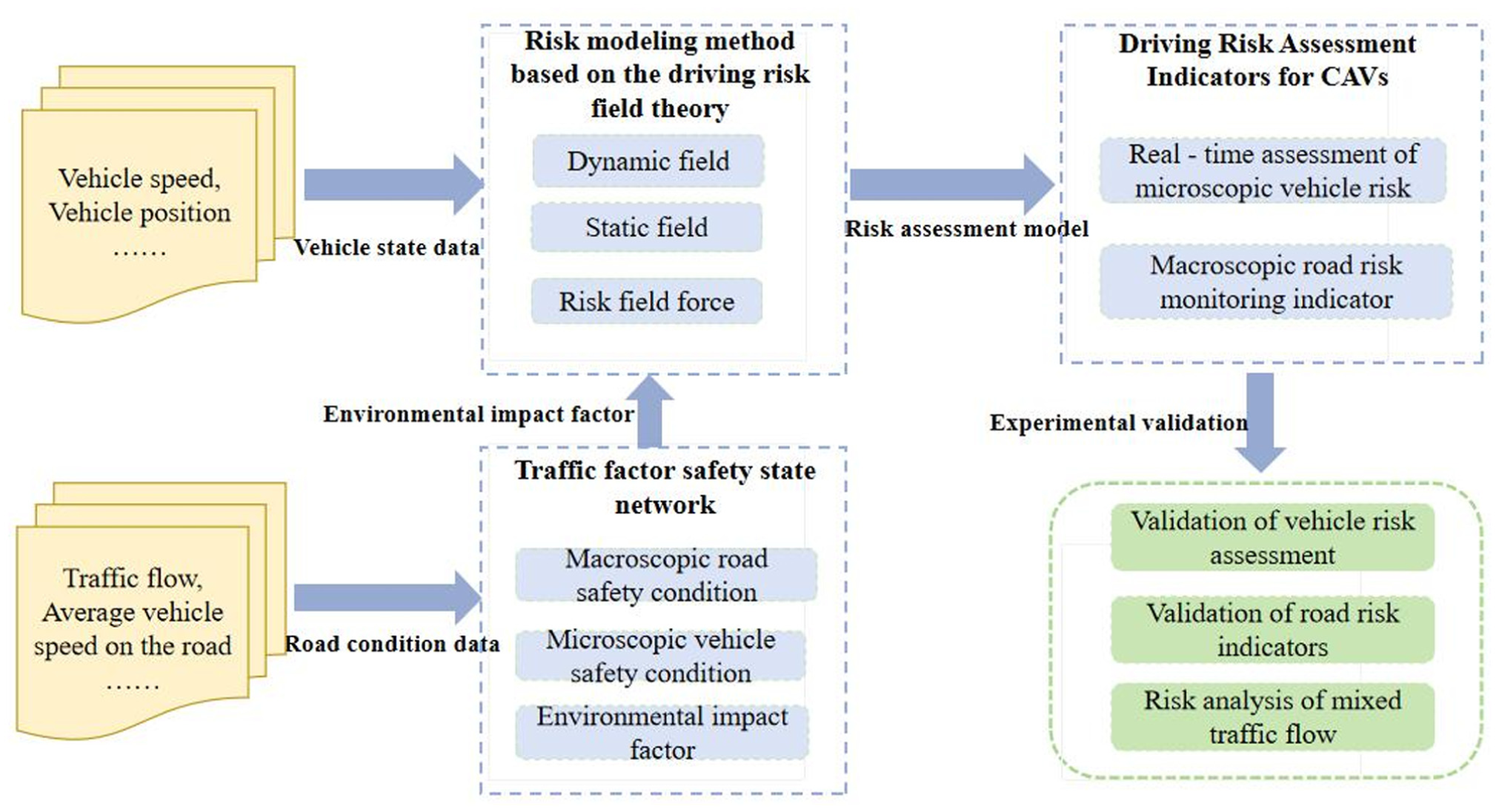
Framework diagram of the risk assessment method for connected and autonomous vehicles (CAVs).

Risk Modeling Method Based on the Risk Field Theory

This section mainly introduces the driving risk field theory and the driving risk modeling method. We describe the risk field, the static field, the dynamic field, and the definition of risk force.

The Concept of the Driving Risk Field

The field serves as a fundamental mode of matter existence and facilitates the transmission of interactions between objects. From the perspective of physics, the field can be understood as a prediction of the interaction capabilities that an object forms with other surrounding objects in time and space. The risk has similar characteristics to the field, and this risk also has spatiotemporal properties. Therefore, it is possible to consider applying field theory to study driving risk.

The driving risk field, also known as the safety potential field, characterizes the impact of other traffic entities on driving risk (33 –35). According to field theory, this risk can be understood as the force perceived by the driver when a vehicle interacts with other vehicles on the road.

To improve the driving risk modeling method, we design a pseudo-distance that considers the shape of the vehicle, obtains the environmental impact factor through traffic state classification, and uses the driving personality factor to distinguish the intelligence level of CAVs and ordinary vehicles.

The driving risk field can be divided into the “static field” related to stationary objects and the “dynamic field” related to moving objects. Therefore, the driving risk field strength at a certain position can be defined as:

E = E_{s} + E_{d}

(1)

where E is the total driving risk field strength, E_s is the risk field strength generated by all static field sources, and E_d is the risk field strength generated by all dynamic field sources.

Static Field

The static field characterizes the risk impact generated by stationary objects. For these objects, the severity of a collision with the vehicle is associated with the object’s equivalent mass. Concurrently, the likelihood of a collision is related to the distance between the vehicle and the object. Risk can be regarded as the product of the probability of collision and the severity of collision. Drawing on the method of calculating field strength in the electrostatic field, we can define the static field strength as:

E_{s} = k_{1} \frac{M}{{| l |}^{k_{2}}} \cdot \frac{l}{| l |}

(2)

where M is the equivalent mass of the object, l is the pseudo-distance between the point and the risk field source, and k₁ and k₂ are related parameters. In Wang et al. ( 33 ), the researchers believed that the equivalent mass is closely related to the vehicle’s current speed, and they derived the following form:

M = m \cdot (1.566 \cdot 10^{- 14} \cdot v^{6.687} + 0.3345)

(3)

where m is the actual mass of the field source object, and v is the speed of the object. Specifically, for the field source objects in the static field, their speed is 0.

Let the centroid coordinates of the risk source be (a, b), and the coordinates of a certain position be (x, y). Then the actual distance d from that position to the centroid of the risk source is:

| d | = \sqrt{(x - a)^{2} + (y - b)^{2}}

(4)

If the actual distance d is directly used to calculate the risk field strength, it would result in equal risk field strengths at the same distance from the risk source, which is unreasonable in practice. Taking the vehicle shown in Figure 2a as an example, because of the asymmetry of the vehicle shape, the distance relationship between points in different directions and the vehicle body is different. Points A and B are on a circle centered at the vehicle centroid P. Point B is obviously closer to the vehicle body than point A, so the risk level at point B should be higher.

Figure 2.

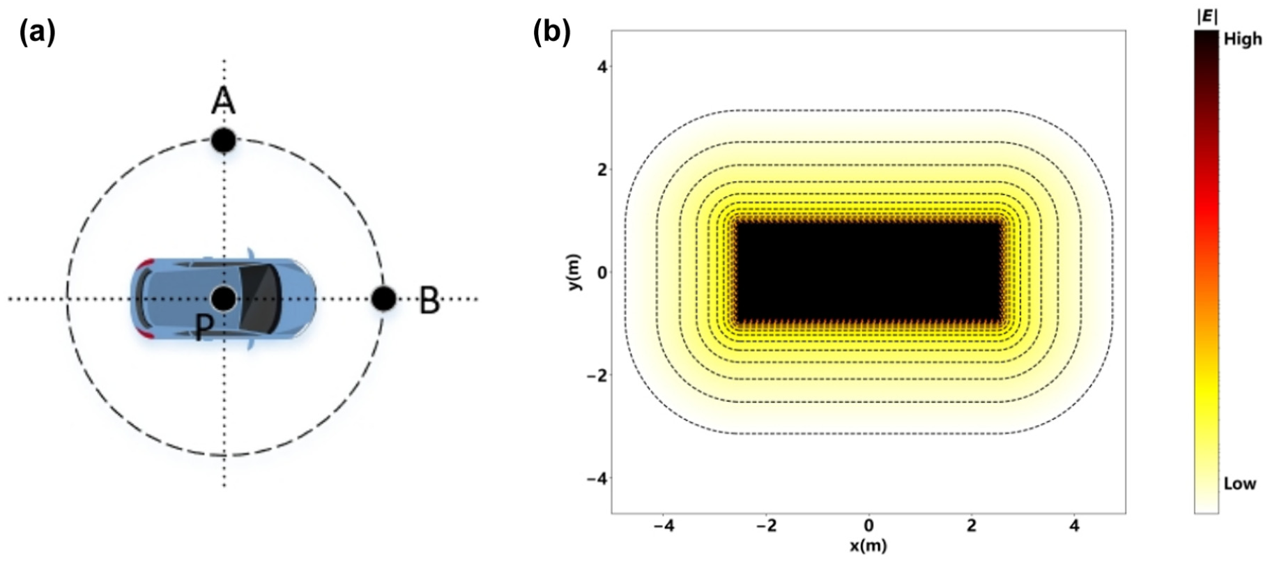
Schematic diagram of the static risk field: (a) display of the vehicle and surrounding location points and (b) distribution of the risk field around the vehicle.

Therefore, our method corrects the distance to a pseudo-distance l, that is the minimum distance from a certain position to the risk field source. This can more accurately reflect the impact of the shape and size of the risk field source on the risk level. Additionally, to prevent numerical instability caused by the pseudo-distance approaching zero in near-collision scenarios (which would cause the risk field intensity to increase sharply), a minimum critical threshold is set for l. In this paper, a threshold of 0.001 m is adopted as an example to ensure computational stability.

For example, the vehicle in the top-view perspective in Figure 2b can be approximated as a rectangle. The distribution lines of the risk field strength around it take on a shape similar to a rounded rectangle, rather than concentric circles. The depth of color represents the strength of the risk field, with darker colors indicating higher risk field strength near the vehicle.

Dynamic Field

The dynamic field characterizes the risk impact generated by moving objects that may collide with the vehicle. Unlike the static field, the driving risk in the dynamic field is also affected by the magnitude and direction of the moving object’s velocity. For example, in Figure 3a, if the vehicle’s velocity is directed horizontally to the right, then at the same distance, the driving risk at point B is greater than that at point A, while the risk at point C is intermediate. Therefore, we can define the dynamic field strength as follows:

E_{d} = k_{1} \frac{M}{{| l |}^{k_{2}}} \cdot \exp (λ v \cos θ) \cdot \frac{l}{| l |}

(5)

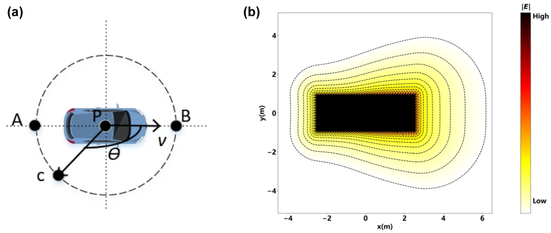
where M is the equivalent mass of the object, l is the pseudo-distance between the point and the risk field source, $λ$ , k₁, and k₂ are related parameters, and θ is the angle between the line connecting the centroid of the object and a certain position and the direction of the moving object’s velocity (as shown in θ in Figure 3a). The cosine function of θ in the formula ensures that the closer a position is to the direction of vehicle movement, the higher the degree of danger.

Figure 3.

Schematic diagram of the dynamic risk field: (a) display of the vehicle and surrounding location points and (b) distribution of the risk field around the vehicle.

As can be seen from Figure 3b, the field strength at the position of the object in the dynamic field is at its maximum, and the distribution range of the risk field in the direction of the object’s movement is wider. This indicates that the risk impact in the direction of the object’s movement is more significant, aligning with the actual risk characteristics of driving.

Risk Field Force

A vehicle located in the driving risk field can be regarded as being subjected to a virtual risk field force. The direction of the force coincides with that of the risk field strength, and this force aims to prevent the vehicle from approaching other objects. The magnitude of the force is determined by the risk field strength, the environment, the vehicle’s own attributes, the vehicle’s motion state, and the characteristics of driving behavior. Therefore, we can define the risk field force as:

F = E \cdot \frac{M}{R \cdot D} \cdot \exp (μ v \cos θ)

(6)

where E is the risk field strength. M is the equivalent mass of the vehicle, µ is a parameter to be determined, and v is the vehicle’s speed. θ is the angle between the direction of vehicle speed and the direction of field strength. The closer the direction of vehicle speed is to the direction of increasing field strength, the higher the likelihood of a collision. R is the environmental impact factor, and D is the driving personality factor.

The environmental impact factor R comprehensively reflects the influence of external elements (such as traffic flow and road infrastructure) on vehicle risk. Based on the TFSSN theory proposed in this paper, different traffic safety states of a given road segment can be identified via clustering methods using macroscopic monitoring data (such as traffic volume and speed). Subsequently, surrogate safety measures (such as time headway) are employed to quantify the overall risk level of the road under each safety state, thereby deriving the corresponding environmental impact factor R for each state.

The driving personality factor D captures the effect of driving styles on risk. Following a similar rationale to that used for the environmental impact factor R, vehicles can be categorized into different driving-style types (such as relatively conservative or aggressive) based on their average operational data over a specific period (such as average speed and average spacing). Then, using surrogate safety measures (such as time headway) over the corresponding period, the average risk level of vehicles with each driving style is estimated, ultimately yielding the driving personality factor D.

Traffic Factor Safety State Network

This section introduces the concept of the TFSSN and proposes a method for classifying traffic safety states.

The Concept of the TFSSN

Highways constitute a vital component of the modern transportation system. By collecting and analyzing highway data, the characteristics and patterns of traffic operation can be revealed. Factors that affect the state of highways not only include obtainable traffic parameters but are also influenced by external factors, such as the environmental impact, that are difficult to directly observe. This has led to the issue of how to measure hidden environmental factors.

This paper extends the traffic factor state network theory (47 –51) to the scenario of road safety assessment. The TFSSN can be understood as a modeling method for analyzing the interrelationships between traffic factors and safety states. There are complex interactions between traffic factors (such as flow, speed, and vehicle position) and traffic safety states. Combined with domain knowledge in the field of transportation, the TFSSN can include the following three basic assumptions:

(1) The state of highways can be divided into macroscopic road states and microscopic vehicle states. Macroscopic road states are usually represented by indicators such as the average traffic volumes and average speed of a section, which are called road factors. The microscopic components are composed of the position and speed of each vehicle, which are called vehicle factors. Environmental impact factors affect both macroscopic and microscopic states, and they constitute a complete transportation system.

(2) The traffic flow operation patterns of highways are embedded in the traffic flow data of the section. Accurately quantifying the impact of these factors through theoretical models is typically challenging. However, rich traffic data can effectively reflect the role of these factors.

(3) There are different numbers of road states in each traffic system. Under different road states, the risk of collision will be different, corresponding to different road safety states. Under the same road safety state, the values of relevant factors are stable, that is, road factors gather within a certain numerical range.

As shown in Figure 4, for the moment t, the macroscopic road safety state is determined by macroscopic road factors (traffic volume, average vehicle speed, etc.) and environmental impact factors. The microscopic vehicle safety state of each vehicle is determined by microscopic vehicle factors (speed, position, etc.) and environmental impact factors. The macroscopic data of the road can be obtained by aggregating the microscopic state data of all vehicles.

Figure 4.

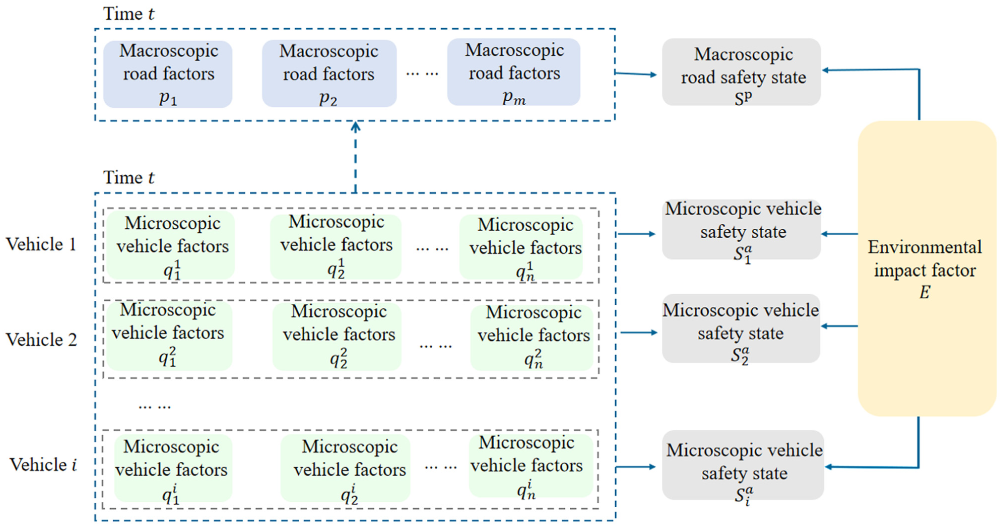
Traffic factor safety state network.

Method for Classifying Macroscopic Road Safety States

Road factors within different numerical ranges correspond to different safety states, that is, under the same road state, road factors often gather within a certain numerical range. Therefore, our method uses EM (Expectation Maximization) algorithm and GMM (Gaussian Mixture Model) to cluster macro-road information, thereby classifying different macroscopic road safety states.

First, effective macro-road information $I$ is extracted from historical traffic data, and the data are processed into a time series with a step length of 5 min:

I = {I^{1}, I^{2}, \dots, I^{i} \dots, I^{n}}

(7)

where $i$ is the sample number, $n$ is the number of samples, $i \in {1, 2, \dots, n}$ , and $I^{i}$ is the macro-road information of the i-th sample:

{F^{i}, V^{i}, \dots}

(8)

$I^{i}$ includes traffic volume $F^{i}$ and average vehicle speed $V^{i}$ of the section. Because of dataset limitations, this study employs speed and flow as representative variables for state classification. Theoretically, however, incorporating more relevant road state features (such as weather conditions and road geometry) would contribute to a more accurate delineation of road safety states.

There are unknown hidden environmental variables in the input samples of the TFSSN. The EM algorithm introduces latent variables to describe the data-generation process, thereby better adapting to different data distributions. By performing maximum likelihood estimation of the model parameters, the algorithm can iteratively obtain clustering results that consider the hidden variables, thereby determining the number of macroscopic road states N:

N = \arg \min_{N} f_{evaluation} (I, N)

(9)

where $I$ is the feature pair dataset composed of traffic volume and average vehicle speed for each time step. $N$ is the number of states, and the value that minimizes the evaluation function $f_{evaluation}$ is taken as the optimal number of state divisions (depending on the evaluation function, it may also be the value that maximizes it).

For real-time macroscopic road data $I_{0}$ , the macroscopic road state $S_{p} (I_{0})$ can be determined by calculating the posterior probability of the road data belonging to each state and selecting the state with the maximum posterior probability. The specific steps are as follows:

(1) For a new feature pair $I_{0}$ , the probability density of the point belonging to each cluster $k$ is calculated using the known mean $μ_{k}$ and covariance $Σ_{k}$ for each cluster state $k$ . If a Gaussian distribution is used as the clustering model, the following formula is applied:

P (I_{0} | k) = \frac{1}{\sqrt{(2 π)^{d} | Σ_{k} |}} \exp (- \frac{1}{2} (I_{0} - μ_{k})^{T} Σ_{k}^{- 1} (I_{0} - μ_{k}))

(10)

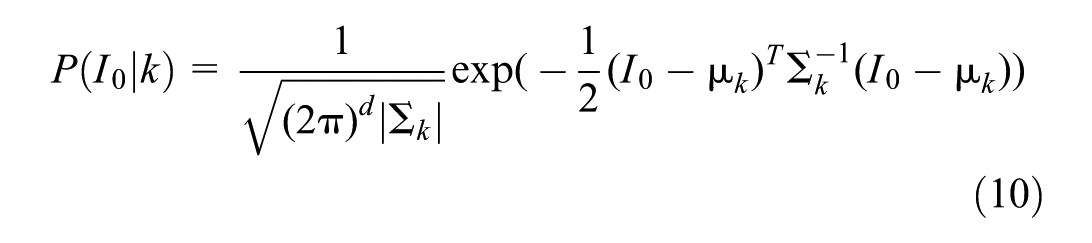
where d is the dimension of $I_{0}$ , and $| Σ_{k} |$ is the determinant of the covariance matrix.

(2) Using Bayes’ theorem, the posterior probability of the new feature pair $I_{0}$ belonging to each cluster k is calculated as:

P (k | I_{0}) = \frac{P (I_{0} | k) P (k)}{P (I_{0})}

(11)

where $P (k)$ is the prior probability of cluster k, $P (I_{0})$ can be obtained by summing the weighted probability densities of all clusters:

P (I_{0}) = \sum_{k} P (I_{0} | k) P (k)

(12)

(3) Finally, the cluster $S_{p} (I_{0})$ with the maximum posterior probability is selected as the category for the new feature pair $I_{0}$ :

S_{p} (I_{0}) = \arg \underset{k}{m ax} P (k | I_{0})

(13)

Driving Risk Assessment Indicators for CAVs

This section designs microscopic vehicle risk assessment indicators VRFI and macroscopic road risk monitoring indicators RRFI, and introduces the specific methods for real-time acquisition of risk assessment indicators from traffic data.

Definition of Risk Assessment Indicators

In the risk field model presented earlier, the magnitude of the risk force can characterize the degree of risk repulsion of the traffic element on a vehicle. Therefore, we can define the sum of the magnitudes of the risk forces experienced by a vehicle as the VRFI for that vehicle.

VRFI = \sum_{i = 1}^{n} | F_{i} |

(14)

where $| F_{i} |$ is the magnitude of the risk field force generated by any risk field source on the vehicle, which can be either a static field force or a dynamic field force.

The development of connected vehicle and sensor technologies makes it possible to obtain the precise trajectories of vehicles in real time, thereby allowing the calculation of the risk field indicator VRFI for each vehicle. The microscopic safety condition of a vehicle describes the risk status of a single vehicle, and changes in the microscopic states of multiple traffic entities can trigger changes in the macroscopic safety condition of the entire traffic flow. Although changes in the risk of a single vehicle occur more frequently and require high-precision real-time risk assessment, the overall road risk is relatively stable over a certain period of time and has lower requirements for time granularity. Therefore, the average risk assessment index of the road over a period of time can be used as the current macroscopic road risk monitoring indicator, that is, the RRFI over a period of time:

RRFI = \frac{\sum_{j = 1}^{N} \frac{\sum_{i = 1}^{n_{j}} {VRFI}_{i}}{n_{j}}}{N}

(15)

where N is the number of times the road risk field index is measured over a period of time, and $n_{j}$ is the number of vehicles on the road at the time of the j-th measurement.

Process for Obtaining Risk Assessment Indicators

As illustrated in Figure 5, the TFSSN theory proposed earlier enables data-driven clustering to identify distinct traffic safety states for a given road segment. By employing SSMs such as time headway, the overall risk level of the road under different safety states can be determined, thereby deriving the corresponding environmental impact factor for each state. Subsequently, by integrating real-time state information of the current vehicle with the aforementioned environmental impact factors and applying the driving risk modeling methodology established earlier, the real-time VRFI can be computed. The microscopic VRFI can be utilized as a standalone indicator, whereas the macroscopic RRFI is derived through the aggregation and averaging of VRFI values. Finally, the RRFI is obtained by calculating the average risk assessment value of all vehicles on the road segment over a specified time period.

Figure 5.

Risk assessment process.

Microscopic vehicle risk assessment indicators provide a reference for real-time vehicle decision-making and intelligent control, such as taking braking or steering measures in emergencies. Meanwhile, based on trajectory prediction algorithms, the overall risk index of different trajectories can be assessed, thereby providing a basis for vehicle trajectory planning.

Macroscopic road risk monitoring indicators can serve as a basis for intelligent road control, such as speed limits or traffic restrictions. In addition, this indicator can be used by traffic management departments as a risk measure for selecting open-test roads for CAVs, and it can also assess the actual operation of CAVs on the road.

Experiments

This section conducts validation experiments for the driving risk assessment method of CAVs. First, the effectiveness of the microscopic vehicle risk assessment indicator VRFI is verified through numerical simulation experiments. Subsequently, the effectiveness of the macroscopic road risk monitoring indicator RRFI is validated by combining real-world highway traffic data with simulation techniques. Finally, the driving risk of mixed traffic flow under different scenarios is analyzed.

Validation of Microscopic Vehicle Risk Assessment Based on Numerical Simulation

To verify the effectiveness of the risk calculation model and risk indicators VRFI proposed in this paper, we conducted numerical simulation experiments. The simulation scenarios included a car-following scenario and a lane-changing scenario. This simulation aims to validate the effectiveness of the proposed risk assessment indicators in general scenarios, rather than focusing on the specific microscopic behavior of vehicles. Therefore, in the numerical simulation experiments, we simplified the behaviors of the vehicles.

We selected several other risk assessment metrics for comparison with VRFI, including the conventional SSM represented by TTC, its enhanced version TTC_mo (Time-to-Collision with Motion Orientation) ( 16 ), and the PFI (Potential Field Indicator) (36 –39) based on safety potential field theory:

TTC: TTC is the most widely used SSM, representing the time required for two vehicles to collide without changing their speeds. Many automotive collision-prevention systems have adopted TTC as a basic danger warning standard indicator. Its definition formula is:

TTC = {\begin{matrix} \frac{x_{2} - x_{1}}{v_{2} - v_{1}}, v_{1} > v_{2} \\ \infty, v_{1} \leq v_{2} \end{matrix}

(16)

where x₂ is the position of the rear of the lead vehicle, x₁ is the position of the front of the following vehicle, v₂ is the speed of the lead vehicle, and v₁ is the speed of the following vehicle.

TTC_mo: This is an indicator specifically designed for CAVs that incorporates the yaw angle of conflict objects, developed as an enhancement to the traditional TTC. The yaw angle represents the orientation of other road users and objects detected by CAV sensors. Through geometric analysis of each detected object’s boundaries, this metric enables better identification of potential risk events by capturing changes in both motion direction and positional relationships.

PFI: This constitutes a microscopic driving risk assessment metric for CAVs based on safety potential field theory, which incorporates the vehicle’s own kinematic state and interactions with the surrounding environment, but does not account for the influence of vehicle dimensions and geometry.

The simulated road is a one-way dual-lane highway with a lane width of 3.5 m. The vehicle length is 5 m, the vehicle width is 1.8 m, and the vehicle mass is 1,500 kg. Referring to previous work (36 –39), the relevant parameters for the risk field calculation model can be set as k₁ = 0.001, k₂ = 2, $λ$ = 0.2, µ = -0.2.

Car-following Scenario Experiment

As shown in Figure 6a, two vehicles are traveling in the same direction in the same lane. The initial distance r₁ between the two vehicles is set to 20 m, and both vehicles have an initial speed of 10 m/s. It is assumed that the lead vehicle begins to decelerate at 2 m/s² to a speed of 6 m/s at the fifth second, and the following vehicle starts to decelerate at 4 m/s² to a speed of 6 m/s at the seventh second.

Figure 6.

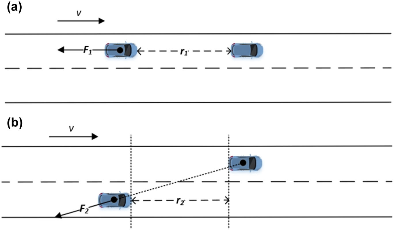
Schematic diagram of the initial states for car-following and lane-changing scenarios: (a) car-following scenario and (b) lane-changing scenario.

According to the driving risk modeling method presented earlier, the following vehicle can be regarded as continuously experiencing a risk repulsion force F₁ from the lead vehicle, thereby obtaining the real-time VRFI for that vehicle.

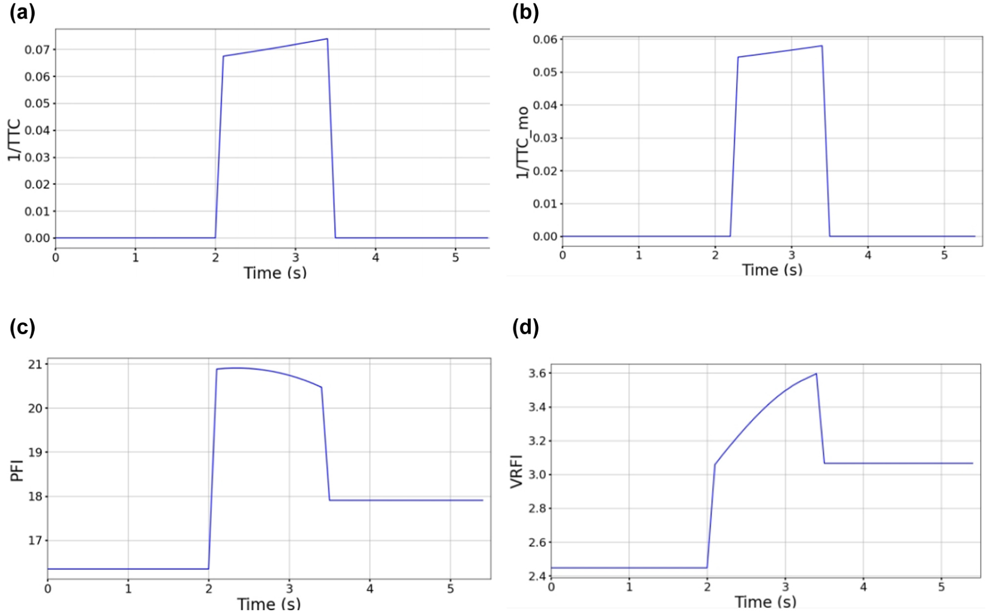
Because of the negative correlation between TTC and TTC_mo with traffic risk, we compared their reciprocal forms with the PFI and VRFI metrics, and plotted the temporal evolution curves of these indicators, as shown in Figure 7. The results demonstrate that the trends of all indicators are generally consistent, collectively reflecting the variation pattern of driving risk over time. TTC_mo primarily represents an improvement over TTC for scenarios such as lane changes and intersections, while exhibiting identical performance to TTC in car-following scenarios.

Figure 7.

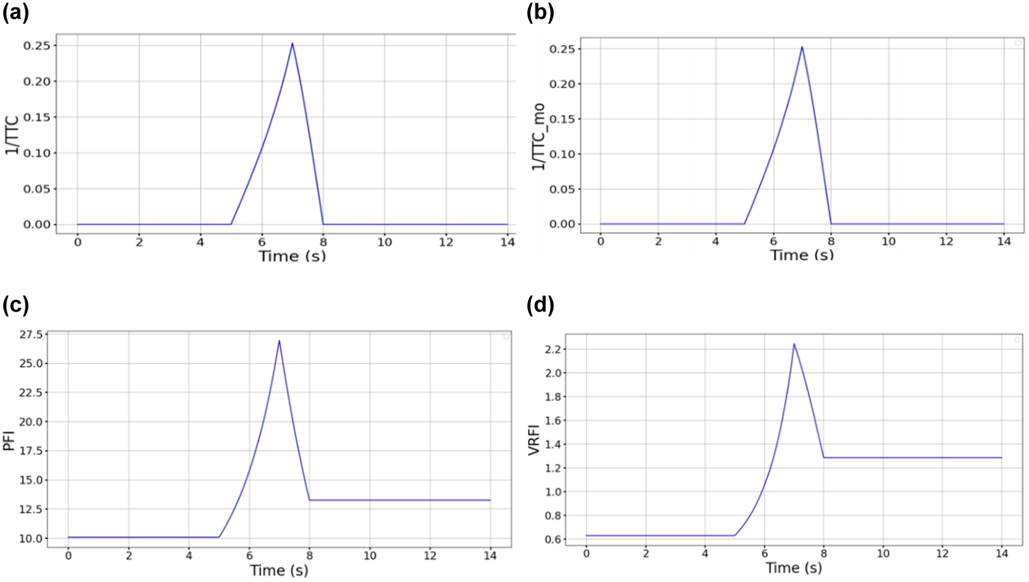
Indicator variation curves under the car-following scenario: (a) 1/TTC variation curve, (b) 1/TTC_mo variation curve, (c) PFI variation curve and (d) VRFI variation curve.

A detailed analysis of Figure 7 reveals that at the fifth second, the leading vehicle abruptly decelerates, resulting in an increased driving risk as all indicators begin to rise. By the seventh second, the following vehicle also initiates deceleration, thereby reducing the driving risk with a corresponding decline observed across all metrics. However, after the eighth second, although both vehicles eventually reach identical velocities causing 1/TTC and 1/TTC_mo to return to their initial levels, VRFI and PFI remain elevated above their baseline values. This discrepancy arises because the reduced inter-vehicle distance is more accurately captured by VRFI and PFI, which consequently reflect the corresponding increase in driving risk.

On the other hand, TTC and TTC_mo can only reflect the probability of vehicle collision but cannot assess the severity of potential impacts. In contrast, the VRFI indicator incorporates equivalent mass to evaluate collision severity, thereby providing a more comprehensive assessment of driving risk levels. Meanwhile, the PFI fails to account for the effects of vehicle size and shape, resulting in relatively lower risk assessment values after the eighth second.

Lane-Changing Scenario Experiment

As shown in Figure 6b, the two vehicles initially travel in the same direction in different lanes. The horizontal distance r₂ between the vehicles along the road direction is set to 10 m, and both vehicles have an initial speed of 5 m/s. It is assumed that the lead vehicle begins to change lanes at a 30° angle to the road direction at the second second and successfully changes to the lane of the following vehicle after 1.4 s.

According to the driving risk modeling method presented earlier, the following vehicle can also be regarded as continuously experiencing a risk repulsion force F₂ from the lead vehicle, thereby calculating the real-time VRFI for that vehicle.

As shown in Figure 8, we plotted the temporal evolution curves of various indicators, which generally maintain consistent trends. Specifically, at the second second, the lead vehicle initiates a lane change, leading to a gradual increase in driving risk. As TTC_mo incorporates the influence of vehicle motion direction and safety zones, it only begins to calculate effective risk values at the 2.3rd second when the lane-changing vehicle intrudes into the host vehicle’s lane. By the 3.4th second, the following vehicle completes the lane change, resulting in reduced driving risk. Because of the decreased inter-vehicle distance after the lane change, both VRFI and PFI successfully capture the corresponding risk elevation, whereas 1/TTC and 1/TTC_mo fail to reflect this variation. Furthermore, during the lane-changing maneuver, the VRFI demonstrates a characteristic gradual risk increase with diminishing vehicle spacing, a feature that PFI fails to adequately represent.

Figure 8.

Indicator variation curves under the lane-changing scenario: (a) 1/TTC variation curve, (b) 1/TTC_mo variation curve, (c) PFI variation curve and (d) VRFI variation curve.

Description of the Advantages of VRFI over Traditional Risk Assessment Indicators

Based on the preceding simulation experiments, the practical significance of VRFI can be qualitatively elaborated from the perspectives of metric definition and application effectiveness. Firstly, TTC and TTC_mo primarily reflect the minimum predicted time to collision between two vehicles. Their assessment is solely based on the collision probability corresponding to the minimum time to collision, failing to account for collision severity. Furthermore, these two indicators are confined to two-vehicle interaction scenarios and are difficult to extend to complex traffic environments involving multiple vehicles. In contrast, VRFI approximates the influence of collision severity by introducing the concept of equivalent mass and can be readily applied to multi-vehicle interaction scenarios.

Secondly, although PFI, based on safety potential field theory, can assess overall risk in complex scenarios, its modeling process does not adequately incorporate the influence of vehicle size and geometry. However, in actual driving, differences in vehicle size and shape directly affect whether collisions occur. VRFI addresses this aspect to enhance safety for long-tail or complex scenarios.

With advancements in sensor and vehicle networking technologies, intelligent and connected vehicles can obtain increasingly rich and accurate data about their own status and the surrounding environment. Traditional indicators such as TTC and TTC_mo struggle to fully utilize these data for more precise risk assessment, whereas VRFI can better integrate and leverage multi-source status information and is inherently suitable for multi-vehicle systems. Although VRFI involves increased computational load, it enables more comprehensive risk assessments by making fuller use of available data. This contributes to further enhancing the safety and intelligence of connected vehicles, thereby promoting their widespread adoption.

Simulation Validation of the Macroscopic Road Risk Monitoring Indicator

To verify the effectiveness of the proposed macroscopic road risk monitoring indicator RRFI, this paper collected real-world highway traffic data and used simulation techniques to reproduce the vehicle trajectories on the road. By classifying the safety state of the road and calculating the RRFIs, we analyzed the changes in road risk and ultimately validated the correlation between the RRFI and the probability of accidents to some extent.

Data Description

To validate the effectiveness of the proposed road risk assessment indicators, trajectory data and accident data for vehicles on the road every day are needed, but such data are extremely difficult to obtain. Therefore, we collected real-world traffic data (including loop detector data and collision accident data) and combined simulation techniques to obtain approximate vehicle trajectory data.

Drawing on previous work ( 56 , 57 ), this paper selected a section of the northbound I-880 Expressway in Alameda County, East Bay, California, USA. As shown in Figure 9, the section is 1456 m long, and is equipped with four sets of loop detectors that can collect average speed and traffic volume. The data from the loop detectors come from California’s Caltrans PeMS system, whereas the collision accident data are from the Transportation Injury Mapping System (TIMS).

Figure 9.

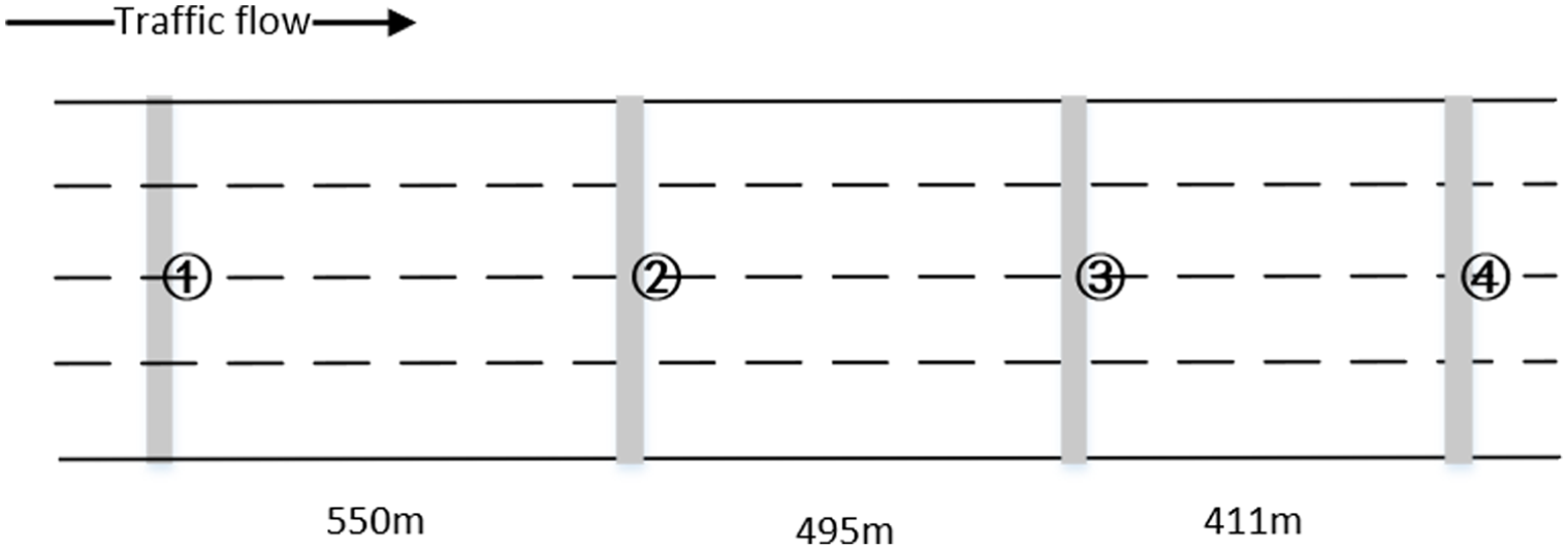
Schematic diagram of the selected highway section.

We used the simulation software SUMO (Simulation of Urban MObility) to reproduce the traffic flow. SUMO is an open-source traffic simulation software mainly used for urban traffic flow simulation. First, we established a road map based on the actual road alignment and ensured that the distribution of loop detectors was consistent with reality. This paper used the Intelligent Driver Model (IDM) model to simulate car-following behavior and used the calibrator in SUMO to calibrate the simulated traffic flow. The calibrator can dynamically adjust traffic parameters such as traffic volume and speed according to the actual measurements from loop detectors, so that the simulated traffic flow characteristics are as close as possible to the real-world data.

The variation curves of the simulated and real-world speed and flow data collected by loop detectors are shown in Figure 10. It can be seen that the simulated traffic volume and average speed are generally consistent with the real-world traffic data obtained from the Caltrans PeMS system. After statistical analysis, the average error rate of the simulated speed is 7.90%, and the average error rate of traffic volume is 13.29%, with errors basically controlled within 15%. Therefore, the simulated data can be considered valid.

Figure 10.

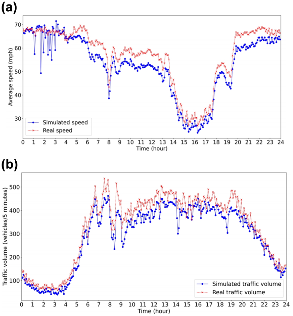
Comparison curves of simulated and real-world traffic flow characteristics: (a) comparison curves of simulated and real-world average speed and (b) comparison curves of simulated and real-world traffic volume.

Classification of Macroscopic Road Safety States

Based on the TFSSN theory presented earlier, we can classify the macroscopic road safety states using the historical traffic data of the section. We selected the average speed and traffic volume collected by the loop detectors in this section from August 23 to August 27, 2021, as the macroscopic road information. Subsequently, we used the EM algorithm based on Gaussian mixture distribution to cluster the road data to mine the environmental impact factors, thereby obtaining the classification results of road safety states.

To determine a reasonable number of macroscopic road safety state categories, this paper selected the Davies–Bouldin Index (DBI), Dunn Index (DI), and Silhouette Coefficient (SC) to evaluate the clustering results. A smaller DBI and a larger DI and SC indicate better clustering performance.

We normalized the historical traffic data and clustered it into two to five states. Table 1 shows the clustering performance indicators after clustering with different numbers of states. It can be seen that when the number of clusters is three, the DBI is the smallest, whereas the DI and SC are the largest, indicating the best clustering performance. Therefore, we chose to classify the road traffic safety state into three categories, and Figure 11 shows the clustering results.

Table 1.

Comparison of Clustering Metrics with Different Numbers of Categories

Evaluation index	Cluster 2 categories	Cluster 3 categories	Cluster 4 categories	Cluster 5 categories
DBI	0.649	0.459	0.532	0.655
DI	0.563	0.636	0.572	0.512
SC	1.302	1.645	1.186	1.095

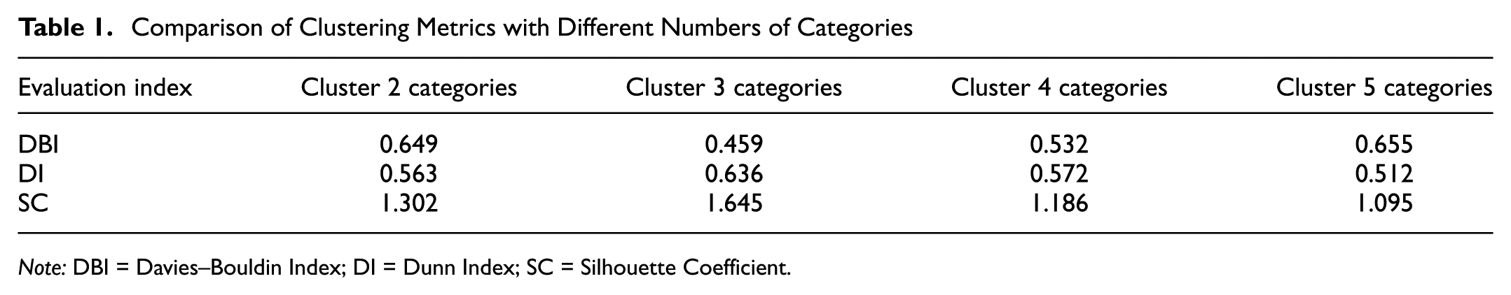
Note: DBI = Davies–Bouldin Index; DI = Dunn Index; SC = Silhouette Coefficient.

Figure 11.

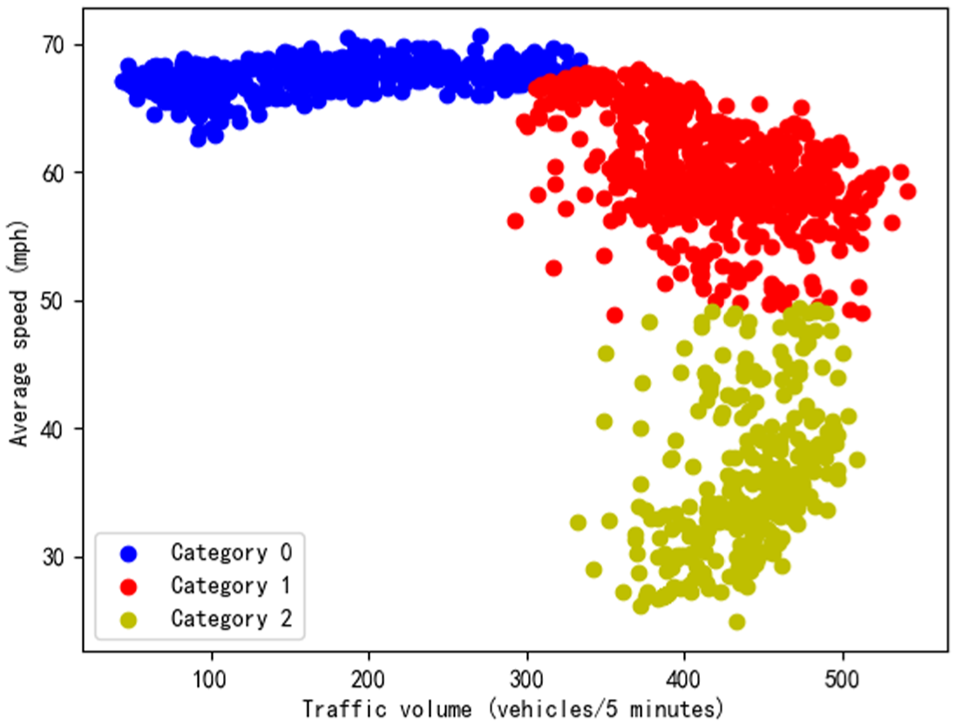
Clustering results of macroscopic road data.

After clustering, we obtained the traffic state sets for different dates within each time period. Considering the inherent volatility and periodicity of traffic data, we used a voting method to correct the traffic states within each time period. Figure 12 shows the modified classification results of macro-traffic conditions.

Figure 12.

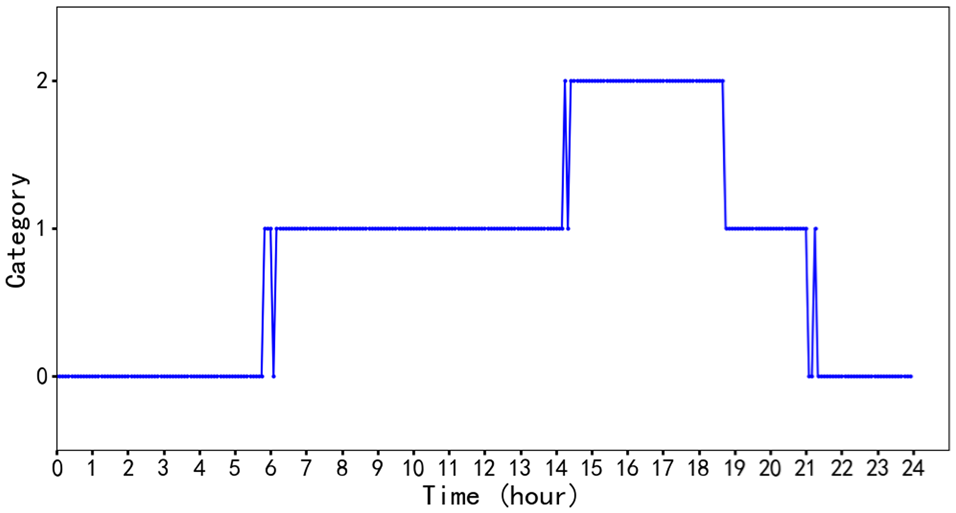
Correspondence between macroscopic road safety states and time periods.

Combining Figure 11 and 12, it can be seen that when the observation time is around 21:00 to 06:00, the macroscopic road safety condition belongs to category 0. During this period, the traffic volume is low and the average speed is high, reflecting the actual late-night (early morning) hours. When the observation time is around 06:00 to 14:30 and 19:00 to 21:00, the macroscopic road safety condition belongs to category 1. During this period, the traffic volume is high and the average speed is fast, corresponding to the off-peak hours in reality. When the observation time is around 14:30 to 19:00, the macroscopic road safety condition shifts to category 2. During this period, the traffic volume is high and the average speed is slow, reflecting the peak hours in reality. Although there is some fluctuation during the short period of state transition, overall, the state remains relatively stable over a period of time.

According to the risk indicator acquisition method presented earlier, we can study the road risk under different traffic safety conditions using SSMs (such as headway) to obtain the environmental impact factors under different traffic safety conditions. Therefore, we statistically analyzed the headway of the simulated traffic flow and obtained the average headway corresponding to categories 0, 1, and 2 as 6.76 s, 3.50 s, and 2.56 s, respectively. As a smaller average headway usually corresponds to a higher driving risk, the environmental impact factor will be smaller. We assumed that the environmental impact factor for category 0 is 1, and then the environmental impact factors for categories 1 and 2 can be calculated as 3.50/6.76 and 2.56/6.76, respectively. Finally, the environmental impact factors corresponding to categories 0, 1, and 2 are 1, 0.52, and 0.38, respectively.

Variation Patterns of Road Risk

Following the classification of road safety states for the target segment, the traffic data from August 26, 2021, were utilized as a case study. First, by incorporating the environmental impact factors corresponding to different road safety states, the microscopic VRFI for each vehicle at each time step was calculated. Subsequently, the macroscopic RRFI was derived by averaging the VRFI values of all vehicles on the road segment over 5 min intervals. Finally, the temporal variation of the macroscopic RRFI throughout that day was plotted, as shown in Figure 13.

Figure 13.

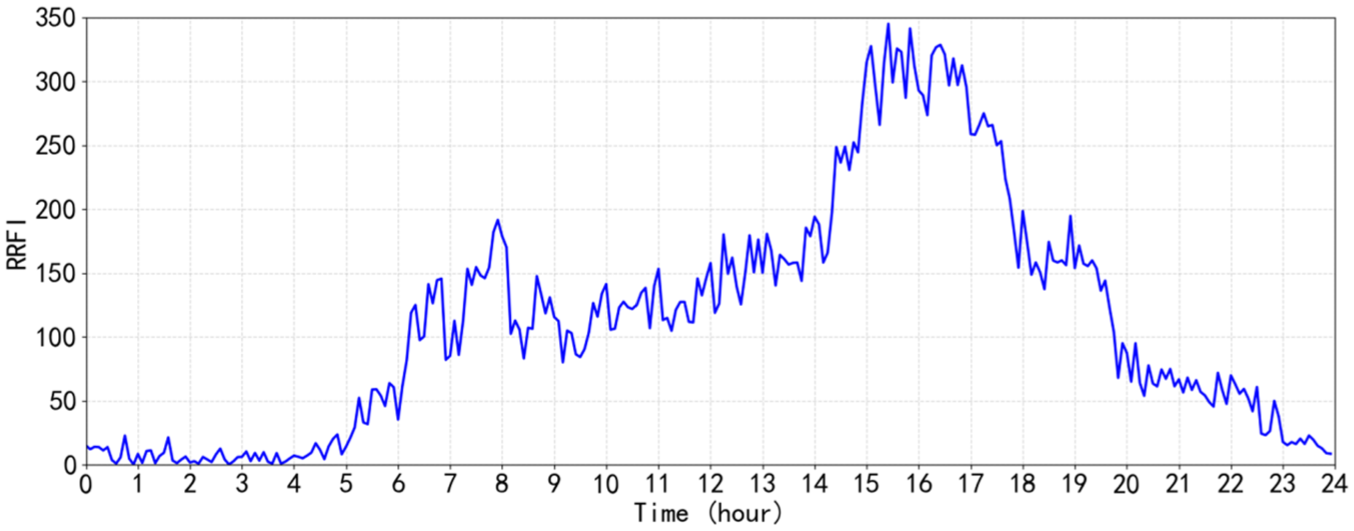
Variation curve of the road risk field indicator.

As can be seen from Figure 13, the risk value of this section is low during the evening hours from 21:00 to 06:00 and high during the peak hours from around 14:30 to around 19:00. According to the TIMS system, an accident occurred on this section at around 17:30 that day, which coincided with the high-risk period.

To further verify the effectiveness of the proposed RRFI, we statistically analyzed the road risk distribution characteristics under different traffic safety conditions and plotted a boxplot (see Figure 14). The median values of the road risk indicators for categories 0, 1, and 2 were 12.19, 95.27, and 222.83, respectively, showing a clear increasing trend, and the degree of data dispersion also increased. This indicates that the RRFI can effectively distinguish different traffic safety conditions.

Figure 14.

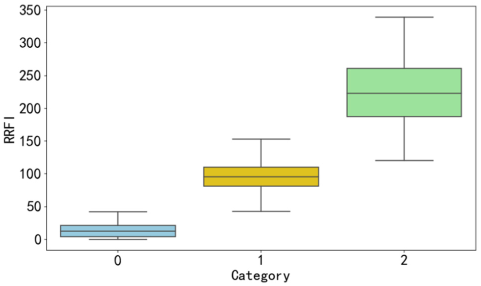
Boxplot of road risk field indicator distribution under different traffic safety conditions.

According to the TIMS system, thirteen accidents were recorded in this section during the working days of 2021. We obtained the real-world traffic data before the accidents from the Caltrans PeMS system and reproduced the traffic scenarios through simulation, finally calculating the RRFI 5 min before the accidents and plotting the distribution (see Figure 15). It can be seen that the RRFI before the vast majority of accidents is higher than the average risk value of this section, and the distribution is more concentrated in the high-risk area, all of which are in category 2 of the macroscopic road safety state. This shows that the RRFI has the potential for road traffic risk monitoring and early warning.

Figure 15.

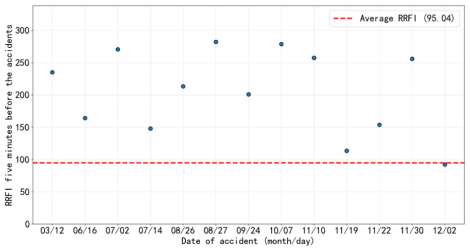
Distribution of road risk field indicators before accidents.

Impact Analysis of Accidents Based on Simulation Experiments

In the proposed risk model, the primary role is played by the microscopic vehicle risk assessment indicator VRFI, which incorporates specific vehicle state data. The macroscopic road risk monitoring indicator RRFI represents an aggregated average of VRFI. VRFI is significantly influenced by the states of both the subject vehicle and surrounding vehicles. Consequently, the impact of abnormal traffic states on VRFI is manifested through changes in these vehicle states. To better demonstrate the effects of such abnormal traffic conditions, this study simulates accident impacts through simulation experiments.

The experiment utilized 2 h of traffic flow data (15:00–17:00) from the road dataset described earlier. A traffic accident was assumed to occur at 16:00, with normal traffic conditions resuming after 30 min. To realistically simulate the accident’s impact on traffic flow, a vehicle was set to remain stationary for 30 min in the SUMO simulation environment, approximating the reduction in local capacity caused by an actual accident.

As shown in Figure 16, we compared the average speed and flow profiles of the road under normal conditions and under accident scenarios. A noticeable decline in both average speed and flow is observed at 16:00, with a return to normal levels after approximately 30 min, demonstrating that the simulation effectively replicates the impact of an accident on traffic flow.

Figure 16.

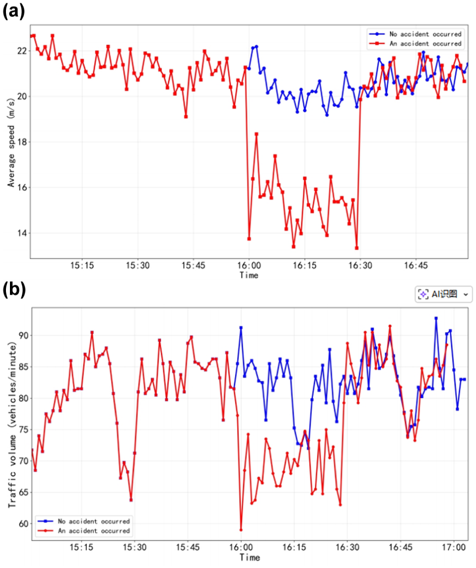
Changes in average speed and traffic flow of road sections under no accident and accident conditions: (a) change in average speed and (b) change in traffic flow.

Subsequently, the temporal variation of the RRFI is plotted in Figure 17. The results indicate a significant increase in the RRFI for approximately half an hour following the accident at 16:00. This trend aligns with the evolution of traffic congestion caused by the incident, demonstrating that the RRFI effectively captures changes in road risk resulting from such unexpected events. These findings confirm that the proposed macroscopic road risk monitoring indicator RRFI possesses the capability to warn of elevated risks induced by traffic accidents.

Figure 17.

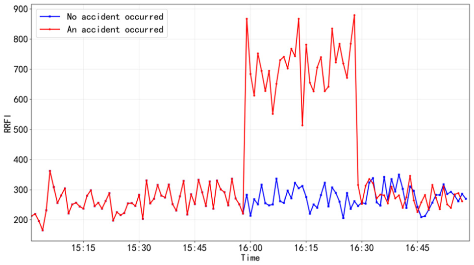
Road risk field indicator change of road section under no accident and accident conditions.

Validation of Risk Assessment Based on the Real-world Vehicle Trajectory Dataset

To further validate the effectiveness of the proposed risk assessment metrics, we computed and analyzed the VRFI and RRFI indices using the real-world HighD ( 58 ) trajectory dataset.

The HighD dataset is a widely recognized German highway naturalistic driving vehicle trajectory dataset, specifically designed for safety validation of highly automated driving systems. Data were collected from an aerial perspective using camera-equipped drones, providing high-precision vehicle positioning and motion information. For this study, we selected data from a three-lane highway segment near Cologne, Germany, which includes thirty-seven recording periods (each approximately 15 min) containing approximately 80,000 vehicle trajectories. The segment covers a road length of 420 m with a truck proportion of about 23%.

Validation of Microscopic Vehicle Risk Assessment

As illustrated in Figure 18, we initially extracted the trajectory data of vehicle 1011 and its preceding vehicle 1005 over a 27 s period from Recording 25 of the dataset. The variation patterns of both vehicle speeds and the microscopic vehicle risk assessment indicator VRFI were subsequently analyzed. As shown in Figure 19, the preceding vehicle initially decelerates, prompting the following vehicle to perceive the potential hazard and subsequently reduce its speed. However, as the speed of the preceding vehicle remains lower than that of the follower, the VRFI value continues to increase, indicating a progressively higher driving risk for the following vehicle. Around the 18 s mark, the speeds of the two vehicles equalize, and the VRFI value reaches a local maximum. Beyond 18 s, the speed of the preceding vehicle exceeds that of the following vehicle, resulting in a gradual decrease in the VRFI value, which signifies a reduction in the driving risk for the following vehicle. These observations demonstrate that the VRFI metric effectively captures the dynamic evolution of the following vehicle’s driving risk.

Figure 18.

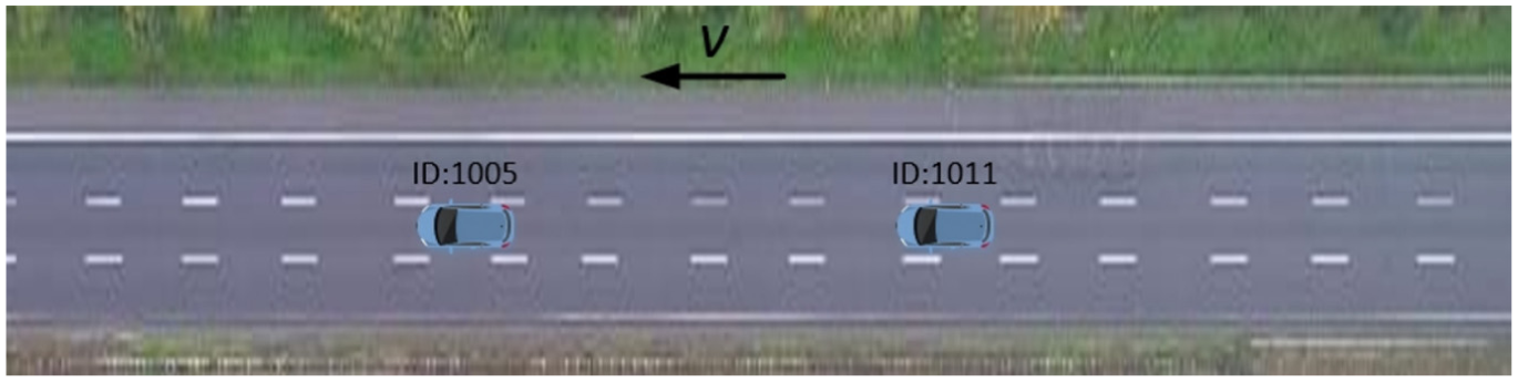
Schematic diagram of the selected highway segment from the HighD dataset.

Figure 19.

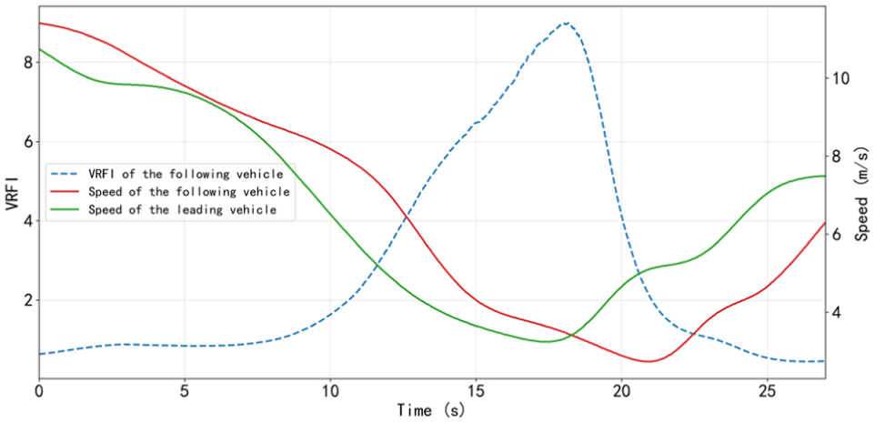
Speed and vehicle risk field indicator (VRFI) profiles of the leading and following vehicles.

Validation of the Macroscopic Road Risk Monitoring Indicator

To validate the proposed macroscopic road risk monitoring indicator RRFI using the HighD dataset, this study first classified the macroscopic safety states of the road segment based on the TFSSN theory. By acquiring the road’s average speed and flow data, a clustering analysis was performed using the EM algorithm based on a GMM, yielding the optimal clustering result as shown in Figure 20. It can be observed that the road states are categorized into three distinct safety levels: Category 0 represents conditions with relatively low traffic demand, characterized by higher average speeds and lower traffic volumes; Category 2 corresponds to high traffic-demand conditions, featuring both higher average speeds and elevated traffic volumes; Category 1 reflects congested road conditions, marked by lower average speeds and reduced traffic flow.

Figure 20.

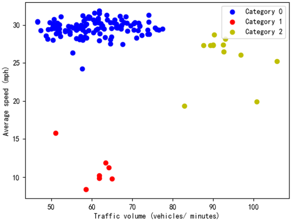
Classification of macroscopic safety states for the road segment based on clustering algorithm.

As the HighD dataset lacks actual crash data, we adopted the frequency of severe conflicts as a surrogate measure for road safety evaluation, defining events with the TTC of less than 1.5 s as severe conflicts ( 57 ). As summarized in Table 2, this study calculated and compiled the average RRFI values and related metrics for the road segment under different macroscopic safety states.

Table 2.

Average Road Risk Field Indicator (RRFI) and Related Data Under Different Safety States for the Selected Road Segment

Category	Average traffic volume (vehicles/minute)	Average speed (m/s)	Average number of conflicts per minute	Average RRFI
0	60.65	29.72	0.28	9.95
1	60.81	11.02	3.17	55.49
2	84.81	26.35	0.75	21.07

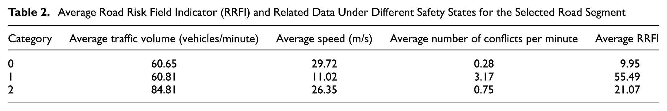
An analysis of the data in Table 2 reveals that Category 0 represents free-flow conditions with low traffic demand, exhibiting the lowest frequency of conflicts and the highest overall road safety level, which corresponds to the lowest average RRFI value. Category 2 represents relatively unimpeded conditions under high traffic demand, characterized by a moderate conflict frequency and an intermediate level of overall road safety, resulting in a medium average RRFI value. In contrast, Category 1 corresponds to congested conditions, showing the highest frequency of conflicts and the lowest overall safety level, consequently yielding the highest average RRFI value. These findings demonstrate that the RRFI metric effectively discriminates between different road safety states, and its variation pattern aligns well with the observed conflict frequency, thereby confirming its capability to reflect risk levels across varying road safety conditions.

Analysis of Macroscopic Risk of Mixed Traffic Flow Under Different Conditions

For a long time in the future, CAVs and manually driven vehicles are likely to coexist for a long period, forming a mixed traffic group. Therefore, the road risk assessment of mixed traffic flow has also become a research focus. In this section, this paper used the designed macroscopic road risk assessment method to analyze the risk characteristics of mixed traffic flow under different traffic volumes, penetration rates of CAVs, and driving styles.

Road Traffic Driving Risk under Different Traffic Volumes

Taking the road section in the earlier experiment as an example, we set 50% of the vehicles as CAVs using the CACC (Cooperative Adaptive Cruise Control) model, and the remaining 50% of the vehicles as ordinary vehicles using the IDM. Meanwhile, the traffic volume was set to 0.5, 1, and 1.5 times the original volume to investigate the changes in the RRFI under different traffic conditions for mixed traffic flow.

As can be seen from Figure 21, the larger the traffic volume, the higher the RRFI value overall, and the more dispersed the data distribution. The median values of the RRFI under traffic volumes of 0.5, 1, and 1.5 times are 20.33, 43.98, and 52.78, respectively. When the traffic volume increases from low (0.5 times the original volume) to medium (1 times the original volume), the RRFI rises significantly, especially during the off-peak and peak hours of the day.

Figure 21.

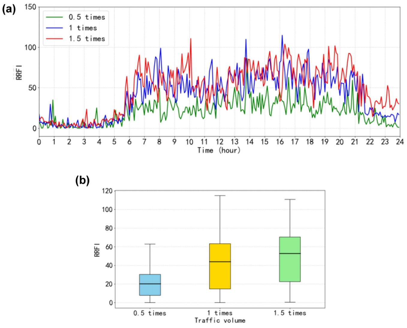
Road risk field indicators (RRFIs) of mixed traffic flow under different traffic volumes: (a) variation curves of the RRFIs and (b) boxplot of RRFI distribution.

Macroscopic Road Risk under Different CAV Penetration Rates

The popularization of CAVs is an ongoing process. We analyzed the impact of different CAV penetration rates on road traffic and plotted the bar charts of the average RRFI value and average travel time under different penetration rates, as shown in Figure 22.

Figure 22.

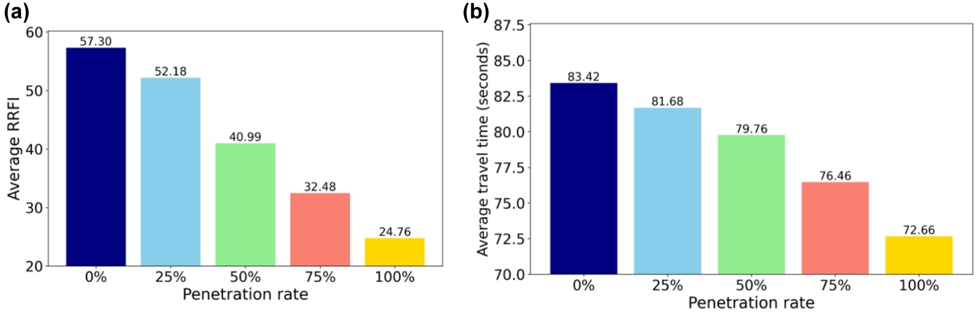
Road traffic conditions under different connected and automated vehicle penetration rates: (a) average road risk field indicators (RRFIs) and (b) average travel time.

As can be seen from Figure 22, the higher the CAV penetration rate, the lower the average RRFI value of the section, and the average travel time also decreases accordingly. The average RRFI value of the road with a penetration rate of 100% is about 57% lower than that of the road with a penetration rate of 0%, and the average travel time on the road is reduced by about 13%. This indicates that the popularization of CAVs can effectively improve the safety and efficiency of road traffic. The macroscopic road risk assessment method presented in this paper offers a novel approach for real-time evaluation of the overall risk in mixed traffic flow and provides a reference for traffic management departments to predict the operation of CAVs on the road.

Road Traffic Driving Risk under Different Driving Styles

Driving style directly influences the microscopic driving characteristics of vehicles. For instance, conservative drivers typically tend to maintain a larger time headway from the preceding vehicle, whereas aggressive drivers accept a shorter time headway. To investigate the impact of different driving styles on traffic flow risk indicators, this study configured three parameter sets for the CACC and IDM models as examples, corresponding to conservative, moderate, and aggressive driving styles. The specific parameter configurations are shown in Table 3. The parameter selection was primarily based on Shen et al. ( 59 ), focusing on two key parameters closely related to driving style: desired time headway (tau) and minimum gap at standstill (minGap). Specifically, the conservative driving style corresponds to larger values of tau and minGap, whereas the aggressive driving style adopts relatively smaller values.

Table 3.

Parameter Configurations of the Models under Different Driving Styles

Driving style	Tau (s)	minGap (m)
Conservative	1.5	1.5
Moderate	1.0	1.0
Aggressive	0.5	0.5

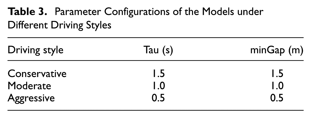
As can be seen from Figure 23, the RRFI values under the conservative driving style are slightly lower, whereas those under the aggressive driving style are relatively higher, with the distinction becoming more pronounced under higher traffic flow conditions. The median RRFI values for conservative, moderate, and aggressive driving styles are 46.56, 51.95, and 59.07, respectively. Moreover, the distribution of RRFI values under the aggressive driving style exhibits greater dispersion. Compared with the moderate style, the RRFI under the conservative style is reduced by 10.38%, whereas under the aggressive style it increases by 13.71%. These results indicate that a conservative driving style contributes to lower overall traffic flow risk, whereas an aggressive driving style leads to higher overall traffic flow risk.

Figure 23.

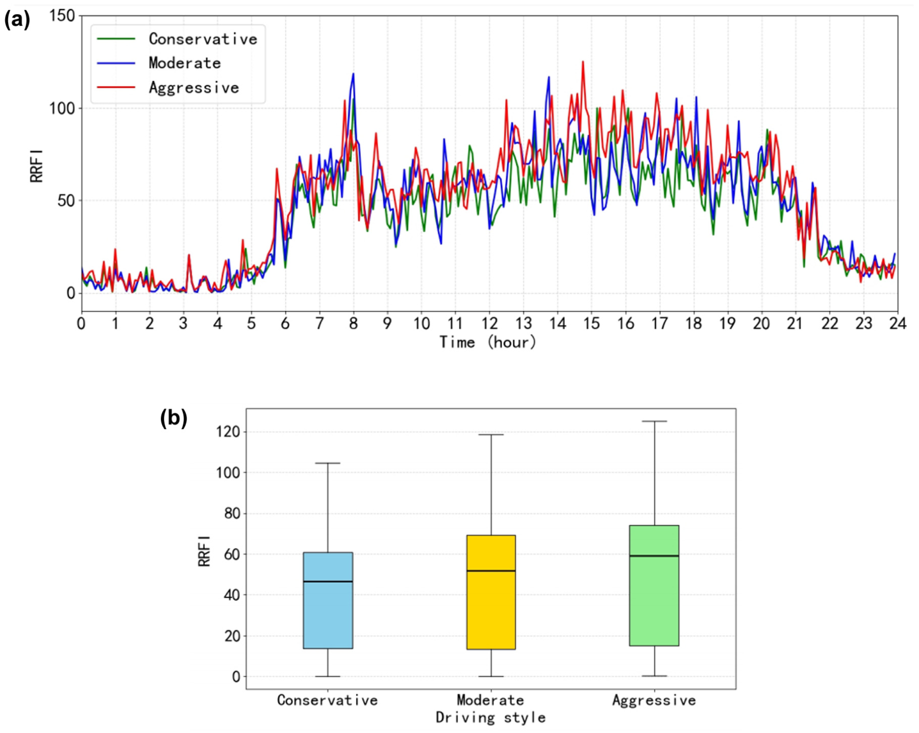
Road risk field indicator (RRFI) values of mixed traffic flow under different driving styles: (a) variation curve of RRFI values and (b) boxplot of RRFI value distribution.

Conclusion

This paper first mined the environmental impact factors hidden in road data based on the TFSSN theory and modeled driving risk based on the driving risk field theory, thereby defining the driving risk assessment indicators for CAVs, including the microscopic vehicle risk assessment indicator VRFI and the macroscopic road risk monitoring indicator RRFI. Subsequently, the rationality of the microscopic vehicle risk assessment indicator VRFI was verified through numerical simulation experiments. Meanwhile, the effectiveness of the macroscopic road risk monitoring indicator RRFI was validated based on real-world traffic data using simulation techniques. Finally, we explored the impact of different traffic volumes and CAV penetration rates on the overall risk characteristics of mixed traffic flow. The experimental results show that the reduction of traffic volumes and the increase of CAV penetration rates can effectively reduce the overall road risk.

The experiments proved that the use of domain knowledge and data-driven methods can effectively classify traffic safety conditions and mine environmental impact factors. The driving risk assessment indicators based on the risk field theory can effectively assess the driving risk of both microscopic vehicles and macroscopic roads. These methods provide new ideas for real-time vehicle risk assessment and road risk monitoring, thereby providing a theoretical basis for intelligent vehicle decision-making at the microscopic level and intelligent traffic control at the macroscopic level.

Because of practical limitations, this paper only conducted experimental validation in a simulation environment. Future research can consider verifying the actual effects in real-world road environments. Moreover, the current penetration rate of CAVs is relatively low, resulting in a lack of sufficient safety data for CAVs. Therefore, the specific parameters in the proposed risk assessment model and statistical verification based on sufficient data can be optimized and adjusted based on richer vehicle safety data in the future. Meanwhile, designing intelligent vehicle decision-making algorithms and road control strategies based on the proposed risk assessment method can be one of the future research directions.

Future Work

The current low penetration rate of CAVs has resulted in a scarcity of CAV safety data, which constrains the model’s validation capabilities in real-world scenarios. With ongoing advancements in sensor and connectivity technologies, it is becoming increasingly feasible to acquire more comprehensive data on the relationship between accidents and vehicle states. Consequently, future work could focus on optimizing and calibrating the specific parameters in the risk assessment model using richer vehicle safety datasets, followed by statistical validation based on sufficient data.

As this study primarily focuses on the overall risk of macroscopic traffic flow and the environmental impact factors under different macroscopic road states, the driving personality factor at the microscopic level has been treated in a simplified manner. Future work can be dedicated to an in-depth investigation of accurate quantification methods for the driving personality factor and its impact on risk.

Furthermore, because of current data limitations, this study only employed speed and flow as the basis for road state classification in the experimental validation. As data-acquisition channels continue to diversify, future research could incorporate additional road state factors (such as weather conditions, road geometry) to better account for the influence of other environmental factors.

Footnotes

Author contributions

The authors confirm contribution to the paper as follows: study conception and design: Long Wang, Weibin Zhang; data collection: Long Wang, Yu Zhang, Ziqi Yan; analysis and interpretation of results: Long Wang; draft manuscript preparation: Long Wang, Weibin Zhang, Yu Zhang, Ziqi Yan. All authors reviewed the results and approved the final version of the manuscript.

Declaration of Conflicting Interests

The authors declared no potential conflicts of interest with respect to the research, authorship, and/or publication of this article.

Funding

The authors disclosed receipt of the following financial support for the research, authorship, and/or publication of this article: This research was sponsored by the National Natural Science Foundation of China (Grant 71971116).

ORCID iDs

Long Wang

Weibin Zhang

Yu Zhang

Ziqi Yan

Data Accessibility Statement

Some or all data, models, or code that support the findings of this study are available from the corresponding author by request.

References

Zhang

World Health Organization Releases Global Status Report on Road Safety 2018. Chinese Journal of Disaster Medicine, Vol. 7, No. 2, 2019, p. 100.

Lin

Fang

Zhao

Modeling Traffic Flow Mixed with Automated Vehicles Considering Dynamic Safety Distance. Transportation Research Record: Journal of the Transportation Research Board, 2025, 2679, No. 10: 840–854.

Chen

Luo

Multiple-Factors Aware Car-Following Model for Connected and Autonomous Vehicles. Transportation Research Record: Journal of the Transportation Research Board, 2021. 2676, No. 2: 649–662.

Yang

Wang

Y. P.

Yuan

Z. Z.

Yin

Y. H.

Guo

M. Z.

Identification of Dynamic Traffic Crash Risk for Cross-Area Freeways Based on Statistical and Machine Learning Methods. Physica A: Statistical Mechanics and Its Applications, Vol. 595, 2022, p. 127083.

Zhao

Liu

Bao

Understand the Impact of Traffic States on Crash Risk in the Vicinities of Type A Weaving Segments: A Deep Learning Approach. Accident Analysis & Prevention, Vol. 159, 2021, p. 106293.

Wang

Liu

Zhang

Development of a Real-Time Crash Risk Prediction Model Incorporating the Various Crash Mechanisms across Different Traffic States. Traffic Injury Prevention, Vol. 16, No. 1, 2015, pp. 28–35.

Lee

Peng

Evaluation of Automotive Forward Collision Warning and Collision Avoidance Algorithms. Vehicle System Dynamics, Vol. 43, No. 10, 2005, pp. 735–751.

Jia

Y. H.

J. P.

An Improved Car-Following Model Considering Variable Safety Headway Distance. Physics Essays, Vol. 27, No. 4, 2014, pp. 616–619.

Wang

J. Q.

Wang

H. P.

Liu

J. X.

Intersection Vehicle Driving Assistance System Based on Vehicle-to-Infrastructure Communication. China Journal of Highway and Transport, Vol. 26, No. 4, 2013, pp. 170–175.

10.

Zhang

Zou

Xie

Wang

Modeling Car-Following Behaviors Using a Driving Style–Based Bayesian Model Averaging Copula Framework in Mixed Traffic Flow. Computer-Aided Civil and Infrastructure Engineering, Vol. 40, No. 21, 2025, pp. 3316–3332.

11.

Ngoduy

Zou

Sun

Modeling Car-Following Behaviors Considering Driver Heterogeneity: A Multi-Regime Stochastic Framework. Transportation Research Part C: Emerging Technologies, Vol. 179, 2025, p. 105282.

12.

Tang

Zou

Xie

Zhang

Comparing Car-Following Behavior Patterns of Human-Driven Vehicles and Autonomous Vehicles in a Mixed Traffic Environment. IEEE Transactions on Intelligent Transportation Systems, Vol. 26, No. 5, 2025, pp. 6814–6830.

13.

Zou

Zhu

Xie

Zhang

Multivariate Analysis of Car-Following Behavior Data Using a Coupled Hidden Markov Model. Transportation Research Part C: Emerging Technologies, Vol. 144, 2022, p. 103914.

14.

Jiang

Lang

Chen

Zhang

Wang

Zhang

Zou

A Dynamic Dual Optimization Method for Safe Lane Changing in Autonomous Driving. Transportmetrica A: Transport Science, 2025, pp. 1–33. https://doi.org/10.1080/23249935.2025.2497887

15.

Cheng

Zhang

Chen

Zou

Analysis of Lane-Changing Conflict Between Cars and Trucks at Freeway Merging Sections Using UAV Video Data. Journal of Transportation Safety & Security, Vol. 15, No. 9, 2023, pp. 943–961.

16.

Ortiz

F. M.

Costa

L. H. M. K.

Sammarco

M. D. M.

Road Traffic Safety Assessment in Self-Driving Vehicles Based on Time-to-Collision with Motion Orientation. Accident Analysis and Prevention, Vol. 191, 2023, pp. 107172.1–107172.15.

17.

Lee

Rouphail

Enhanced Crash Frequency Models Using Surrogate Safety Measures from Connected Vehicle Fleet. Transportation Research Record: Journal of the Transportation Research Board, 2023. 2678, No. 5: 463–478.

18.

Gore

Chauhan

Easa

Arkatkar

Traffic Conflict Assessment Using Macroscopic Traffic Flow Variables: A Novel Framework for Real-Time Applications. Accident Analysis & Prevention, Vol. 185, 2023, p. 107020.

19.

Yuan

Huang

Wang

Sun

Using Traffic Flow Characteristics to Predict Real-Time Conflict Risk: A Novel Method for Trajectory Data Analysis. Analytic Methods in Accident Research, Vol. 35, 2022, p. 100217.

20.

Yuan

Huang

Wang

Sun

Wang

Application of Explainable Machine Learning for Real-Time Safety Analysis toward a Connected Vehicle Environment. Accident Analysis & Prevention, Vol. 171, 2022, p. 106681.

21.

Mogyorósi

Szénási

Laufer

Fuzzy-Based Road Accident Risk Assessment. Mathematics, Vol. 12, No. 8, 2024, p. 1144.

22.

Ali

Haque

M. M.

Mannering

Assessing Traffic Conflict/Crash Relationships with Extreme Value Theory: Recent Developments and Future Directions for Connected and Autonomous Vehicle and Highway Safety Research. Analytic Methods in Accident Research, Vol. 39, 2023, p. 100276.

23.

Yang

Xie

Bai

Liu

Enhancing Safety and Efficiency of Signal Intersections: A Part-Time Protected Right-Turn Signal Control for Straight-Right Lane in Connected Environment. Physica A, Vol. 661, 2025, p. 130378.

24.

Kavianpour

Haghighi

Sheykhfard

Das

Fountas

Oshanreh

M. M.

Assessing the Risk of Pedestrian Crossing Behavior on Suburban Roads Using Structural Equation Model. Journal of Traffic and Transportation Engineering (English Edition), Vol. 11, No. 5, 2024, pp. 853–866.

25.

Saunier

Miranda-Moreno

Evaluation of Conventional Surrogate Indicators of Safety for Connected and Automated Vehicles in Car Following at Signalized Intersections. Transportation Research Record: Journal of the Transportation Research Board, 2025. 2679, No. 2: 1118–1133.

26.

Yang

Ying

Xie

Bai

An Integrated Potential Safety Hazard Assessment Framework in Connected Car-Following Scenario. Accident Analysis and Prevention, Vol. 216, 2025, p. 108010.

27.

Wang

Yeo

Paiva

A. R.

Goodman

J. P.

Utke

Delle Monache. Dynamic Risk Assessment for Autonomous Vehicles from Spatio-Temporal Probabilistic Occupancy Heatmaps. Accident Analysis & Prevention, Vol. 222, 2025, p. 108226.

28.

Olfati-Saber

Flocking for Multi-Agent Dynamic Systems: Algorithms and Theory. IEEE Transactions on Automatic Control, Vol. 51, No. 3, 2006, pp. 401–420.

29.

Byrne

Naeem

Ferguson

Improved APF Strategies for Dual-Arm Local Motion Planning. Transactions of the Institute of Measurement and Control, Vol. 37, No. 1, 2015, pp. 73–90.

30.

A Unified Perspective on Traffic Flow Theory, Part I: The Field Theory. In ICCTP 2011: Towards Sustainable Transportation Systems ( Yin

Wang

, eds.), American Society of Civil Engineers, Reston, VA, 2011, pp. 4227–4243.

31.

A Unified Perspective on Traffic Flow Theory, Part II: The Unified Diagram. In ICCTP 2011: Towards Sustainable Transportation Systems ( Yin

Wang

, eds.), American Society of Civil Engineers, Reston, VA, 2011, pp. 4244–4263.

32.

Lei

Zhao

Chen

A Novel Ellipsoidal Safety Potential Field Model for Quantifying Driving Risk. Transportmetrica A: Transport Science, 2025, pp. 1–30. https://doi.org/10.1080/23249935.2025.2522361.

33.

Wang

The Driving Safety Field Based on Driver–Vehicle–Road Interactions. IEEE Transactions on Intelligent Transportation Systems, Vol. 16, No. 4, 2015, pp. 2203–2214.

34.

Wang

Zheng

Driving Safety Field Theory Modeling and Its Application in Pre-Collision Warning System. Transportation Research Part C: Emerging Technologies, Vol. 72, 2016, pp. 306–324.

35.

Wang

J. Q.

Concept, Principle, and Modeling of Driving Risk Field Based on Human-Vehicle-Road Collaboration. China Journal of Highway and Transport, Vol. 29, No. 1, 2016, pp. 105–114.

36.

L. H.

Gan

Mao

P. P.

Ran

Vehicle Car-Following Model Based on Safety Potential Field Theory in Intelligent Connected Environment. China Journal of Highway and Transport, Vol. 32, No. 12, 2019, pp. 76–87.

37.

Gan

Ran

Dynamic Driving Risk Potential Field Model under the Connected and Automated Vehicles Environment and Its Application in Car-Following Modeling. IEEE Transactions on Intelligent Transportation Systems, Vol. 23, No. 1, 2020, pp. 122–141.

38.

Gan

Ran

Risk Perception and the Warning Strategy Based on Safety Potential Field Theory. Accident Analysis & Prevention, Vol. 148, 2020, p. 105805.

39.

Gan

Zhou

Ran

A Novel Lane-Changing Model of Connected and Automated Vehicles: Using the Safety Potential Field Theory. Physica A: Statistical Mechanics and Its Applications, Vol. 559, 2020, p. 125039.

40.

Cui

H. R.

H. Z.

Modeling Method for Autonomous Driving Risk Field Considering the Complexity of Operating Environment. Modern Transportation and Metallurgical Materials, Vol. 3, No. 4, 2023, pp. 57–68.

41.

Wang

Sun

Safety Risk Assessment for Autonomous Vehicle Road Testing. Traffic Injury Prevention, Vol. 24, No. 7, 2023, pp. 652–661.

42.

Cheng

Zhu

Feng

Yang

Zhang

Chen

Driving Safety Risk Analysis and Assessment in a Mixed Driving Environment of Connected and Non-Connected Vehicles: A Systematic Survey. IEEE Transactions on Intelligent Transportation Systems, Vol. 26, No. 5, 2025, pp. 5747–5781.

43.

Kwak

H. C.

Kho

Predicting Crash Risk and Identifying Crash Precursors on Korean Expressways Using Loop Detector Data. Accident Analysis & Prevention, Vol. 88, 2016, pp. 9–19.

44.

Ding

Abdel-Aty

Zheng

Wang

Traffic Flow Clustering Framework Using Drone Video Trajectories to Identify Surrogate Safety Measures. arXiv preprint arXiv:2303.16651, 2023.

45.

Huang

Luo

Cao

Wen

Zhong

Learning Multiaspect Traffic Couplings by Multirelational Graph Attention Networks for Traffic Prediction. IEEE Transactions on Intelligent Transportation Systems, Vol. 23, No. 11, 2022, pp. 20681–20695.

46.

Huang

Chen

Fan

Yan

Incorporating Environmental Knowledge Embedding and Spatial-Temporal Graph Attention Networks for Inland Vessel Traffic Flow Prediction. Engineering Applications of Artificial Intelligence, Vol. 133, 2024, p. 108301.

47.

Zhang

Zha

Zhang

Road Section Traffic Flow Prediction Method Based on the Traffic Factor State Network. Physica A: Statistical Mechanics and Its Applications, Vol. 618, 2023, p. 128712.

48.

Zhang

Zha

Gan

DS-TFSN-Based Vehicle Travel Time Prediction Method for Digital Twin System of Freeways. IEEE Transactions on Intelligent Transportation Systems, Vol. 25, No. 12, 2024, pp. 20073–20084.

49.

Gan

Zhang

Dong

Traffic Factor Dual-State Network: A Novel Framework for Spatial–Temporal Traffic Flow Prediction. Transportmetrica A: Transport Science, 2025, pp. 1–36. https://doi.org/10.1080/23249935.2025.2457339

50.

Zhang

Zha

Gan

Wang

Incident Detection for Freeways Based on a Dual-State Traffic Factor State Network. Transportmetrica A: Transport Science, 2025, pp. 1–29. https://doi.org/10.1080/23249935.2025.2460039

51.

Zhang

Feng

Song

Wang

Speed Prediction Based on a Traffic Factor State Network Model. IEEE Transactions on Intelligent Transportation Systems, Vol. 22, No. 5, 2020, pp. 3112–3122.

52.

Feng

Lei

Zhang

Wang

Han

Analysis on Traffic Accident Severity Influenced by Road Environment on Circular Highway. China Journal of Highway and Transport, Vol. 29, No. 5, 2016, pp. 116–123.

53.

Yoshitake

Kawaguchi

Kawamura

Murata

Soma

Shino

The Influence of Traffic Environment on Collision Risk Assessment Based on Right-Turn Driving Behavior at Intersections. International Journal of Automotive Engineering, Vol. 13, No. 1, 2022, pp. 21–28.

54.

Yang

Liu

Zhang

Adanu

E. K.

Penmetsa

Jones

A Machine Learning Approach to Understanding the Road and Traffic Environments of Crashes Involving Driver Distraction and Inattention (DDI) on Rural Multilane Highways. Journal of Safety Research, Vol. 92, 2025, pp. 14–26.

55.

Yang

R. J.

Wang

X. S.

Application of Aggregated Lane Traffic Data from Dual-Loop Detector to Crash Risk Evaluation. Journal of Tongji University (Natural Science Edition), Vol. 44, No. 10, 2016, pp. 1567–1572.

56.

Yan

A Longitudinal Car-Following Risk Assessment Model Based on Risk Field Theory for Autonomous Vehicles. International Journal of Transportation Science and Technology, Vol. 10, No. 1, 2021, pp. 60–68.

57.

Katrakazas

Quddus

Chen

W. H.

A New Integrated Collision Risk Assessment Methodology for Autonomous Vehicles. Accident Analysis & Prevention, Vol. 127, 2019, pp. 61–79.

58.

Krajewski

Bock

Kloeker

Eckstein

The highD Dataset: A Drone Dataset of Naturalistic Vehicle Trajectories on German Highways for Validation of Highly Automated Driving Systems. In 2018 21st International Conference on Intelligent Transportation Systems (ITSC) ( Zhang

W.-B.

Bayen

A. M.

Sánchez Medina

J. J.

Barth

M. J.

, eds.), IEEE, Piscataway, NJ, 2018, pp. 2118–2125.

59.

Shen

Zhou

Wang

Intersection Passing Strategies for Human-Driven and Autonomous Vehicles in Mixed Traffic Using DEA. PLoS One, Vol. 20. No. 4, 2025, p. e0321566.