
Abstract
Understanding the statistical dynamics of traffic speeds at hazardous and non-hazardous locations is essential for effective roadway safety interventions. This study investigates the distinct characteristics of spot speed distributions across six Indian highway segments, including National and State Highways. It uses continuous probability distributions and hypothesis testing to assess the statistical significance of speed differences between hazardous and non-hazardous locations. The analysis is based on observed spot speed measurements, stratified into four data fractions (25%, 50%, 75%, and 100%), obtained using a simple random sampling with replacement approach. Seven continuous probability distributions, including normal, lognormal, gamma, logistic, Weibull, Burr, and generalized extreme value (GEV), have been fitted independently for each location type and data fraction to capture their distributional characteristics. The location, scale, and shape parameters of the models have been estimated using maximum likelihood estimation. However, model adequacy has been confirmed using Akaike Information Criterion (AIC) and Bayesian Information Criterion (BIC) values. Furthermore, a two-sample Kolmogorov–Smirnov test has been conducted to assess the statistical difference in speed profiles between hazardous and non-hazardous locations. The results reveal that the GEV distribution consistently outperforms other models across all locations and data fractions, demonstrating strong parameter stability and model adequacy. Larger data fractions improved model performance and hypothesis testing power, indicating greater distributional robustness. To address the potential effect of vehicle interactions and transient congestion during the observation periods, a modified Kaplan–Meier (KM) framework is used to estimate congestion-adjusted desired speed distributions. The KM-based findings show that hazardous roadway locations exhibit higher desired speed potential and greater upper-tail speed characteristics compared with non-hazardous locations. Interestingly, statistically significant speed differences have been found in nearly all settings, confirming the notion that crash-prone zones exhibit distinct speed dynamics. These findings have significant implications for road safety policy and infrastructure design, as well as the need for location-specific speed management strategies.
Keywords
Introduction and Background
Overspeeding accounts for more than half of all road crash fatalities in low- and middle-income countries, while it accounts for approximately 30% of road fatalities in high-income countries ( 1 – 3 ). In addition, over 67% of road crashes in India occur on straight road segments, highlighting speed as a significant factor in increasing crash frequency ( 4 , 5 ). Therefore, understanding the statistical dynamics of speeding is crucial for identifying hazardous roadway environments and developing effective safety interventions.
Traffic speed assessment is an important aspect of road safety research because it directly affects a driver’s reaction time, braking distance, and the overall crash risk ( 4 ). Statistical speed modeling, encompassing theoretical and simulation-based traffic flow analysis, plays a crucial role in quantifying the stochastic behavior of traffic flow and explaining speed variations across different roadway environments ( 6 ). Previous research has focused on several aspects, including driver-related factors (age, gender, and alcohol consumption) ( 7 , 8 ), road and vehicle-related factors (geometric design, surface quality, vehicle age, and vehicle power) ( 9 , 10 ), and contextual road environment factors (traffic composition, density, prevailing speed, and weather conditions) ( 11 ) that affect speeding behavior of drivers. Researchers have used different statistical methodologies, including structured regression analysis ( 12 ), binary logistic regression ( 13 ), and Tobit models ( 14 ), to examine crash-causality relationships in this research domain. These models usually provide insights into the correlations between speeding, including demographic characteristics, road geometric design features, and enforcement intensity; however, they often fail to fully capture the distributional nature of spot speeds across diverse traffic environments.
Several earlier studies suggest that speed, as a continuous random variable, follows a normal distribution because it is symmetrically distributed around its central value ( 4 , 15 – 18 ). According to Haight and Mosher ( 19 ), lognormal and gamma distributions may more accurately represent speed distributions than normal distributions, because the same function can be used to convert a time–speed distribution into a space–speed distribution. Pillai and Ramanayya ( 20 ) emphasized the need to fit the speed distribution function for each vehicle type because each vehicle has distinct power, acceleration, and deceleration characteristics, resulting in significant speed differences. McLean ( 21 ) found that car speeds generally follow a normal distribution, with coefficients of variation ranging from 0.11 to 0.18 in moderately dense traffic. Some recent studies have shown that, under heterogeneous traffic conditions, observed spot speed distributions often deviate from normality because of interactions among slow- and fast-moving vehicles, weak lane discipline, and variation in driver behavior ( 18 , 22 , 23 ). For example, Harding et al. ( 24 ) found that the inclusion of auto-rickshaws in the traffic flow considerably reduces the average speed of the stream across the traffic volume range. Saha et al. ( 25 ) focused on minimizing inconsistencies in the distributional assumptions of speed data on two-lane highways with mixed traffic, aiming to improve the accuracy of capacity and Level of Service analyses. The findings indicated that Indian traffic patterns show that a normal distribution effectively characterizes the spot speeds of cars, light commercial vehicles (LCVs), and scooters; however, a lognormal distribution holds for bicycles.
More recent research has increasingly focused on fitting continuous probability distribution functions to model traffic speed behavior, particularly under heterogeneous traffic conditions, in parallel to econometric and regression-based approaches ( 4 , 16 , 18 , 26 ). Researchers, such as Mondal and Gupta ( 18 ) and Sarkar and Kumar ( 4 ), have used continuous probability distributions to investigate the distributional characteristics of vehicle speeds, particularly high-speed driving behavior at four-legged signalized and three-legged unsignalized intersections, respectively. Their study results indicate that the generalized extreme value (GEV) and Burr distributions are the most appropriate empirical speed distributions, with the GEV exhibiting the best-fit above 96%. In a mixed traffic scenario, when the proportion of heavy vehicle composition (trucks, buses, and tractors) is below 10%, it adheres to the Weibull distribution; between 10% and 14%, it follows the gamma distribution; between 15% and 20%, it conforms to the GEV distribution; and above 20%, it fits with the Burr distribution. Furthermore, the normal and lognormal distributions are considered the least suitable models. These findings suggest that three-parameter distribution functions outperform their two-parameter counterparts in modeling the range of observed speeds. These functions capture central tendencies and account for variability, skewness, and kurtosis, all of which are essential for understanding extreme speeding behaviors. This is particularly relevant from a safety perspective because rare but extremely high-speed incidents often contribute disproportionately to crash occurrence and severity.
The majority of research investigations have focused on speed analysis across different road settings and traffic scenarios, including urban and rural roads, freeways, and two-lane highways ( 14 , 15 , 17 , 22 , 25 , 27 ). These analyses have largely focused on specific road facility types, such as midblock, signalized, or unsignalized intersections, without a systematic comparison across these roadway facilities for hazardous roadway locations (HRLs) and non-hazardous roadway locations (non-HRLs) ( 28 ). This represents a significant research gap. To the best of the authors’ knowledge, no previous study has conducted a comparative analysis of traffic speed characteristics at HRLs and non-HRLs on rural two-lane highways. An HRL, often termed a “black spot” or “crash hots pot,” is defined as a specific location on the road exhibiting a significantly higher-than-average concentration of crashes, in contrast to non-HRLs that experience minimal crash events ( 29 , 30 ). In real-world traffic systems, HRLs and non-HRLs often coexist in proximity yet exhibit vastly different driving behaviors because of variations in road geometry, roadway environment, traffic enforcement intensity, traffic flow, land use, and driver risk perception ( 31 , 32 ). Therefore, comparing the speed distributions at HRLs and non-HRLs is statistically and practically insightful in determining how crash-prone segments differ from relatively safer roadway segments for vehicular speed behavior. Such a comparative analysis can reveal whether HRLs exhibit distinct distributional features, such as heavier tails, higher variance, or positive skewness, which may indicate extreme speeding behavior, sudden acceleration or deceleration zones, or irregular vehicular interactions ( 4 , 18 ). However, an additional methodological issue arises because spot speed observations collected during field surveys can capture intrinsic driver speed behavior and transient traffic interaction effects, such as vehicle-following or platooning during the measurement window, which can suppress the observed speeds relative to the desired flow conditions. Therefore, differences in observed speed distributions between HRLs and non-HRLs may partly represent interaction-induced suppression rather than true desired speed behavior. To address this concern, this study supplements conventional observed speed distribution analysis with a modified Kaplan–Meier (KM) approach for estimating the desired speed distribution ( 33 , 34 ). By distinguishing interaction-constrained observations from unconstrained observations using headway-based censoring, the KM framework provides a congestion-adjusted representation of speed behavior, offering a more robust basis for comparing speeds across hazardous and non-hazardous roadway segments.
In summary, the motivation for comparing speed distribution between HRLs and non-HRLs stems from the need to: (1) identify behavioral and statistical anomalies associated with crash occurrence; (2) refine model selection for different traffic conditions; and (3) suggest targeted and data-driven safety interventions. Therefore, this study aims to examine whether there is a statistically significant difference in speed behavior between identified HRLs and non-HRLs on rural two-lane highways under mixed traffic conditions. This study combines distribution fitting and hypothesis testing to assess similarities and differences in observed speed characteristics across the two location types. In addition, it employs a KM framework to estimate congestion-adjusted desired speed distributions. The null hypothesis
The structure of this study is as follows: the first section, Introduction and Background, introduces this study by explaining the relevance of traffic speed to road safety and providing a concise background on research on traffic speed distribution modeling. The next section, Methodology, presents the methodology for modeling spot speed distributions, including goodness-of-fit (GoF) evaluation, a hypothesis-testing framework for speed distribution analysis, and a modified KM approach for desired speed estimation. The following section, study area, data collection, and data preparation, presents the study area and field data collection procedures, along with the data stratification approach and data preparation steps for fitting the speed distributions. The subsequent section, analysis and results, describes the analysis and outcomes of hypothesis testing. The next section, discussion, presents a discussion on the key findings and their implications, and the final section, conclusions, provides the conclusions of this study.
Methodology
Speed distribution is an essential feature in traffic flow modeling for different roadway infrastructure facilities, including both signalized and unsignalized intersections on urban and rural roads under homogeneous and heterogeneous traffic conditions ( 35 ). This section investigates the characteristics of speed distributions formulated for spot speed measurements at HRLs and non-HRLs on rural two-lane highways under mixed traffic conditions.
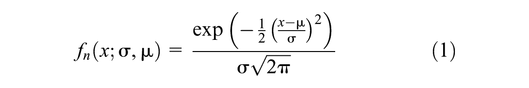
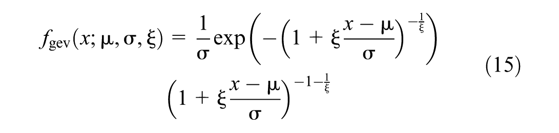
In traffic flow theory, vehicular speed is considered a continuous random variable. Several earlier studies have assumed that speed data follow a normal distribution; however, this assumption often fails in heterogeneous traffic conditions, particularly in mixed traffic scenarios. Different vehicle types and varying driver behavior introduce nonlinearity and asymmetry in speed data. This is further exacerbated in congested traffic environments and at unsignalized intersections because of frequent and uncontrolled traffic maneuvers. These conditions necessitate flexible statistical approaches to capture skewness and extremes in speed data arising from interactions between slow and high-speed driving behaviors. This study used seven continuous probability distribution functions, including normal, lognormal, logistic, gamma, Weibull, Burr, and GEV, to accurately represent the speed data. These parametric distributions are fitted to vehicular speeds using the maximum likelihood estimation method. The empirical distributions investigated are as follows.
Normal Distribution
When the mean
The cumulative distribution function (CDF) of the normal distribution is as follows (Equation 2):

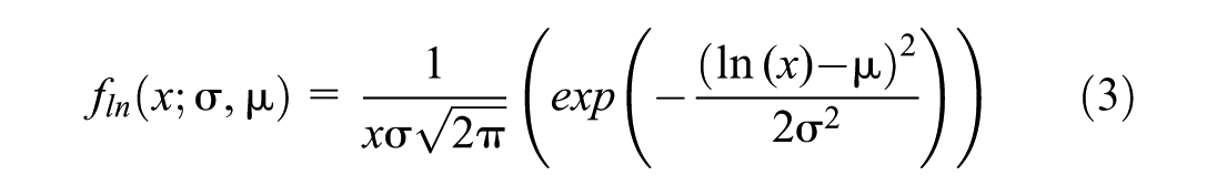
Lognormal Distribution
A random variable x follows a lognormal distribution, which is characterized by two continuous parameters: the scale parameter σ and the location parameter
The CDF of the lognormal distribution is as follows (Equation 4):

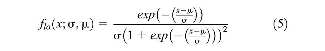
Logistic Distribution
The logistic distribution is a symmetric, bell-shaped distribution similar to the normal distribution, but with heavier tails, making it suitable for various purposes, such as modeling traffic speed when data show moderate skewness and variability. The PDF of this distribution is given as follows (Equation 5):
The CDF of the logistic distribution is as follows (Equation 6):

Gamma Distribution
A random variable x is considered to follow a gamma distribution characterized by two continuous parameters,

The CDF of the Gamma distribution is as follows (Equation 8):
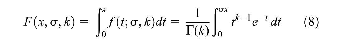
This integral is known as a lower incomplete gamma function; therefore, the CDF can be compactly written as follows (Equation 9):

where

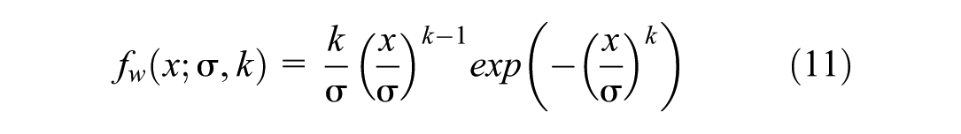
Weibull Distribution
The Weibull distribution is a two-parameter continuous probability distribution widely used in reliability analysis and survival modeling, as well as in traffic speed modeling, because of its flexibility in capturing skewness in speed data. The PDF of this distribution is as follows (Equation 11):
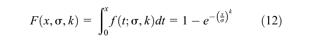
The CDF of the Weibull distribution is expressed as follows (Equation 12):
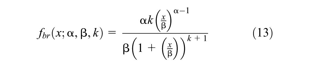
Burr Distribution
The Burr distribution, also known as the Burr Type XII distribution or Singh–Maddala distribution, belongs to the unimodal family of distributions distinguished by diverse shapes. This distribution consists of multiple parameters, including continuous shape parameters
The CDF of the Burr distribution is given as follows (Equation 14):
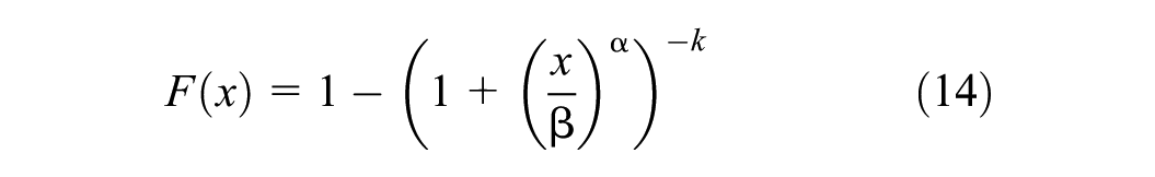
The Burr distribution is appealing for data fitting because of its adaptable scale and location parameters and its flexible shape. A positive skewness number indicates that this distribution is sometimes considered as an alternative to a normal distribution.
GEV Distribution
The GEV distribution is a three-parameter distribution encompassing the Type I (Gumbel), Type II (Fréchet), and Type III (Weibull) extreme value distributions. The GEV distribution consists of three distinct parameters: (1) location
The CDF of the GEV distribution is given as follows (Equation 16):
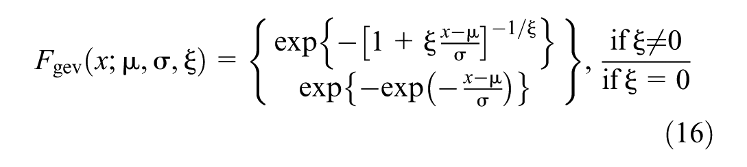
These forms include Type I (Gumbel) when
GoF and Hypothesis Testing Framework for Speed Distribution Modeling
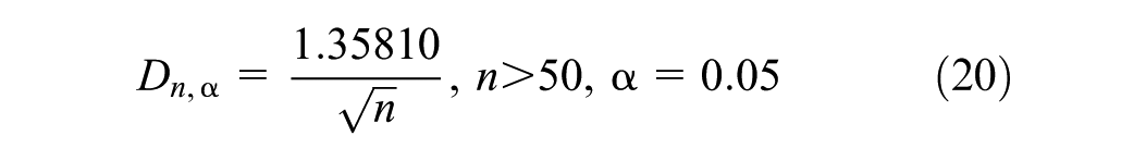
The GoF test is a commonly used approach for determining the distribution function that best fits the empirical speed distribution data. These tests serve as diagnostic tools that determine whether the hypothesized CDF adequately represents the observed speed distribution. In this study, the Kolmogorov–Smirnov (KS) test is used as a GoF test to evaluate the suitability of each distribution in modeling the observed speed data. The KS test measures the maximum absolute difference

The alternative hypothesis

The difference between the ECDF and theoretical CDF is given as follows (Equation 19):

where
k = number of estimated parameters,
n = number of observations, and
The critical value of the KS test can be calculated as follows (Equation 20):
This study aims to validate the hypothesis that there is a statistically significant difference in vehicular speed distributions between HRLs and non-HRLs. A two-sample KS test has been used for hypothesis testing. This test compares the ECDFs of two independent samples of observed spot speed data to determine whether they are derived from the same underlying distribution.
Let:
The hypotheses are defined as follows (Equation 21):

This implies that there is no statistically significant difference between the speed distribution at hazardous and non-hazardous locations. However, the alternative hypothesis is defined as follows (Equation 22):

This implies that there is a statistically significant difference between the speed distribution at hazardous and non-hazardous locations.
The two-sample KS test statistic is calculated as the maximum absolute difference between the two ECDFs. Suppose the test statistic has a p-value significantly lower than the 5% significance level. In that case, the null hypothesis is rejected, indicating that the speed distributions at hazardous and non-hazardous locations are statistically different. The use of the KS test contributes to the statistical validation and reinforces the relevance of distribution-based traffic risk assessment frameworks. In addition, it provides empirical justification for implementing location-specific speed management strategies, targeted enforcement, and road geometric design interventions to improve road safety.
Modified KM Estimation of Desired Speed Distribution
This study uses a modified KM survival analysis approach to distinguish intrinsic speed-choice behavior from speed reduction resulting from vehicle interactions by estimating the desired (free-flow) speed distribution ( 36 ). The KM estimator is particularly suitable for situations with right-censored data, in which the true desired speed of a vehicle is not fully observed because it is constrained by a preceding vehicle. In traffic streams, such censoring occurs when drivers travel in groups or follow slower vehicles, preventing them from attaining their desired speed.
Let

where
The desired speed distribution is estimated using the KM survival function. Let

where

From the estimated survival function, the expected desired speed

Similarly, the second moment of the desired speed distribution is obtained as follows using Equation 26.

which allows the standard deviation of the desired speed distribution to be calculated as (Equation 27),

In addition to the desired speed statistics, two supplementary indicators are reported to characterize traffic interaction effects. The constrained fraction is defined as follows (Equation 28):

where

which provides an empirical upper bound for the observed speed range.
The mean observed speed indicates operating speeds influenced by interactions, while the KM-based desired speed
Study Area, Data Collection, and Data Preparation
Haryana is a relatively small state in India, ranking 21st for area among the 28 states, accounting for less than 1.4% of the country’s landmass ( 38 ). From 2010 to 2020, the state’s road network expanded by 0.27%; however, registered motor vehicle ownership surged by 6.02% during the same time ( 39 , 40 ). The state has witnessed a disproportionately high incidence of fatal crashes, accounting for 3.4% of all crashes and 3.3% of total fatalities across India in 2022 ( 41 ). An investigation into regional crash trends on rural two-lane highways in the Northwest and Southeast regions of Haryana is conducted to facilitate further crash analysis. The selection of this region is motivated by its documented high crash rate, representative traffic composition, and increasing vehicle density. In the southeast region of the state, there are 11 two-lane, undivided rural National Highways (NHs) and State Highways (SHs). Table 1 presents the number of fatalities and the fatality rate (per 100 km) for these 11 highways. Among these highways, it is observed that three SHs (SH 14, SH 16A, and SH 22) and three NHs (NH 709, NH 334B S1, and NH 334B S2) have a high fatality rate (fatalities per 100 km) compared with other highways, as given in Table 1 and shown in Figure 1.
Average Fatality Rate Per 100 km of Two-Lane National Highways (NHs) and State Highways (SH) in Haryana State
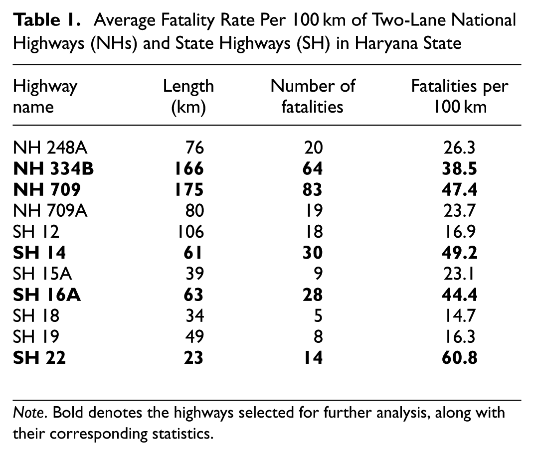
Note. Bold denotes the highways selected for further analysis, along with their corresponding statistics.
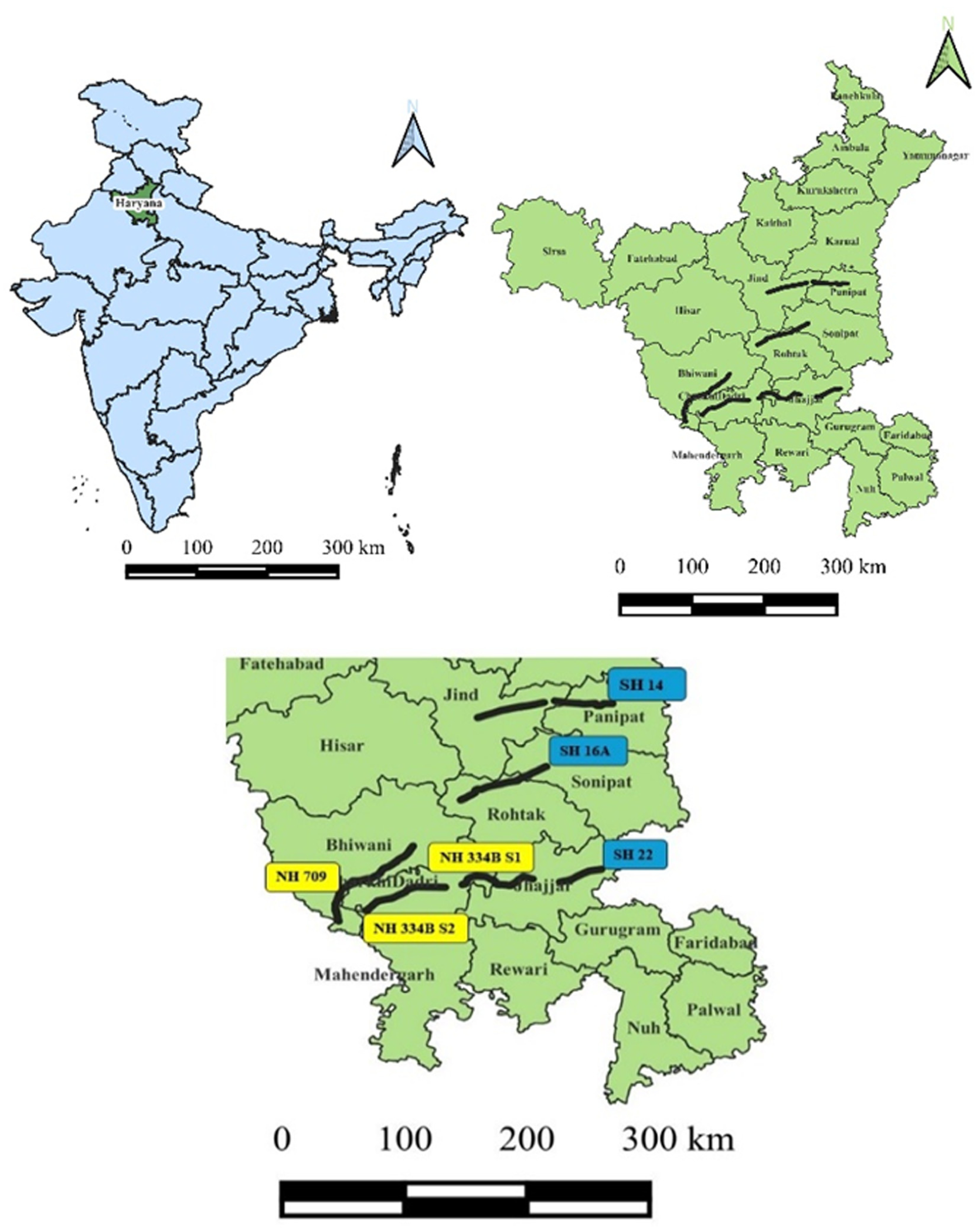
Typical selected National Highways (NHs) and State Highways (SHs) from Haryana, India.
It is important to note that HRLs and non-HRLs were identified based on the outcomes of a previous objective of the authors’ ongoing doctoral research. In that study, HRLs were systematically identified using a negative binomial–Lindley (NB-L) model and a kernel density empirical Bayes (KDEB) approach, using police-reported, georeferenced crash data obtained from the State Police Crime and Criminal Tracking Network System (CCTNS) for 2017–2019. A location was classified as hazardous if its expected crash frequency or density exceeded the top 5% threshold determined in both NB-L and KDEB models. In contrast, locations with crash frequencies or densities consistently below this threshold over the same period were classified as non-hazardous.
Speed data are subsequently collected at these predetermined HRLs and non-HRLs along selected NHs and SHs, including NH 709, NH 334B S1, NH 334B S2, SH 14, SH 16A, and SH 22. The selected locations (HRLs and non-HRLs) consist of straight segments and three-legged unsignalized intersections located on flat terrain, with pavement widths from 7 to 10 m. Each location (e.g., L_1, L_2, and L_3) represents an independent speed measurement point that may be classified as hazardous or non-hazardous and provides location-specific speed behavior influenced by local geometric features, the localized roadway environment, and traffic volume. The locations under investigation are far from the influence of longitudinal gradients and horizontal curves, preventing confounding effects from the gradual acceleration and deceleration of vehicles. At each location, spot speed measurements are obtained for various vehicle types using a Light Detection and Ranging speed gun during a fixed 2 h duration on weekdays between September and October 2024. Data collection was conducted during daylight hours (07:00 a.m.–06:00 p.m.) in clear weather conditions to ensure uniform visibility and to minimize behavioral anomalies associated with adverse conditions. The traffic in the study region is characterized by a heterogeneous environment with poor lane discipline, making speed data collection challenging. To minimize behavioral impedance, the speed of upstream and downstream vehicles is measured at 80–200 m before approaching the conflicting zone, targeting the rear of each vehicle ( 42 ). This ensures that observed speeds reflect natural driving behavior. The observation duration remains uniform across all locations, and the collected samples inherently incorporate variations in traffic composition and operating conditions across peak and non-peak periods within the daytime window.
The 2 h videography survey provides traffic data, categorized into seven distinct vehicle classes: (1) motorized two-wheelers (2W); (2) motorized three-wheelers (3W); (3) standard cars; (4) trucks; (5) buses; (6) tractors; and (7) LCVs, according to the Indo-HCM classification. Tables 2 and 3 present the spatial information for selected hazardous and non-hazardous locations, along with their traffic and speed composition samples.
Location and Traffic Composition at Each Selected Location on the National Highways (NHs)
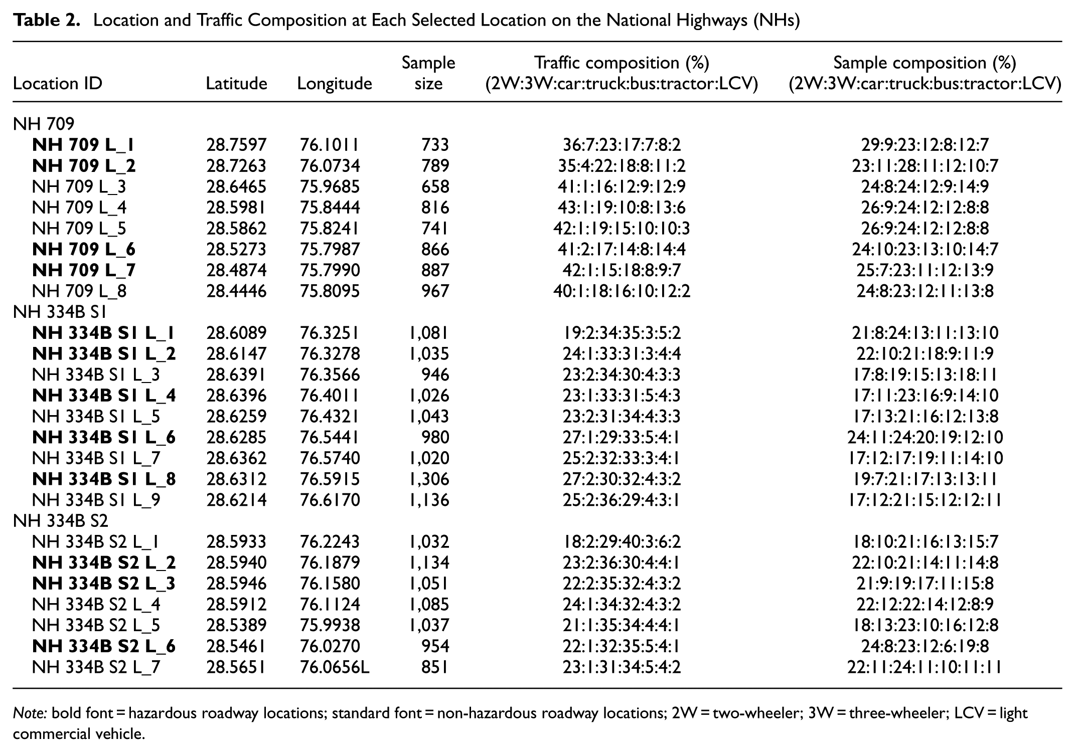
Note: bold font = hazardous roadway locations; standard font = non-hazardous roadway locations; 2W = two-wheeler; 3W = three-wheeler; LCV = light commercial vehicle.
Location and Traffic Composition at Each Selected Location on State Highways (SHs)
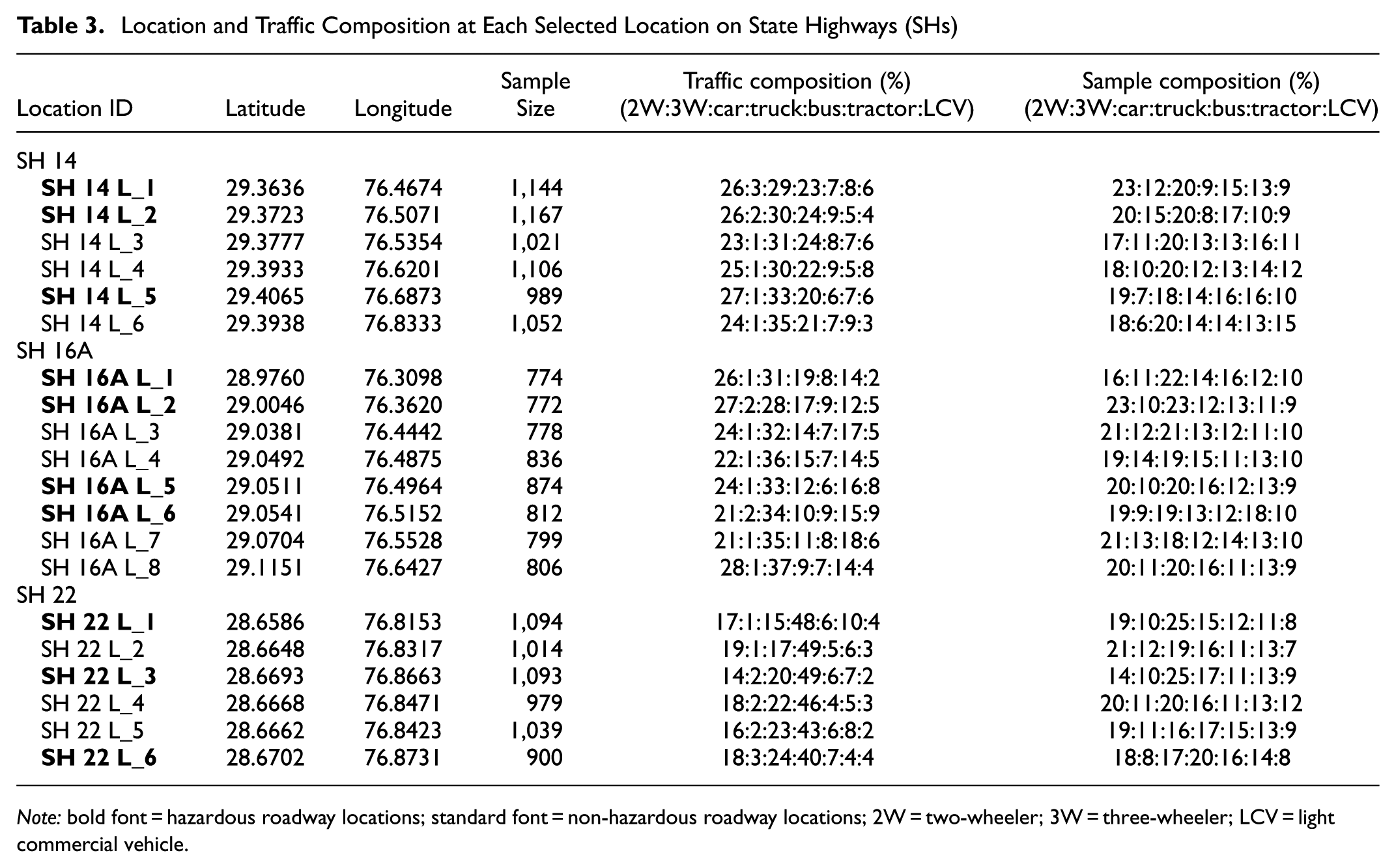
Note: bold font = hazardous roadway locations; standard font = non-hazardous roadway locations; 2W = two-wheeler; 3W = three-wheeler; LCV = light commercial vehicle.
Data Preparation and Stratification for Modeling
The reliability and accuracy of statistical modeling in road safety research critically depend on the rigor of the data preparation process. To examine the sensitivity and robustness of statistical modeling to data availability, the full data set has been systematically divided into four data fractions (25%, 50%, 75%, and 100%) of the total sample size. This stratification is designed to investigate how data granularity affects model performance, parameter convergence, and the reliability of statistical inference. Furthermore, this study adopts a repetition-based sampling framework to evaluate the modeling consistency. For each highway and data fraction (25%, 50%, 75%, and full data set [i.e., 100%]), four data sets (Repetition_1–Repetition_4) are generated using the simple random sampling with replacement approach. The purpose of using several repetitions is twofold. First, these repetitions reinforce the robustness and stability of model fitting methodologies and ensure that any single data set configuration does not unduly influence inferential results. Second, to evaluate the consistency of results across independently drawn subsets of data. This methodological decision improves the generalizability of results and replicability of the findings across diverse traffic scenarios and geographical contexts ( 43 , 44 ).
The prepared data structure, which incorporates variability across location types (i.e., HRLs and non-HRLs), data fractions, repetitions, and highways, enables a comprehensive spot speed analysis based on a stratified experimental design, ensuring the reliability and validity of insights derived from modeling and inferential procedures.
Analysis and Results
Descriptive Statistics of Spot Speeds
Descriptive statistics have been computed for each surveyed location on the NHs and SHs to better understand the basic characteristics and variability of the spot speed data. The key statistical parameters include the sample size, minimum and maximum speed (in km/h), variance, skewness, and kurtosis. Tables 4 and 5 summarize these parameters for HRLs and non-HRLs on NH 709, NH 334B S1, NH 334B S2, SH 14, SH 16A, and SH 22. The Location ID column in the tables includes suffixes, such as L1, L2, and L3 to denote Location 1, Location 2, and Location 3, respectively, along a specific highway segment, as shown in Figure 2. An interactive map of the different locations (e.g., L1, L2, and L3 along NH and SHs), as shown in Figure 2, is available online at: https://parveen4007.github.io/Spot-Speed-Measurements-at-Hazardous-and-Non-Hazardous-Locations-on-National-and-State-Highways/.
Descriptive Statistics for Speed Data at Each Location on National Highways
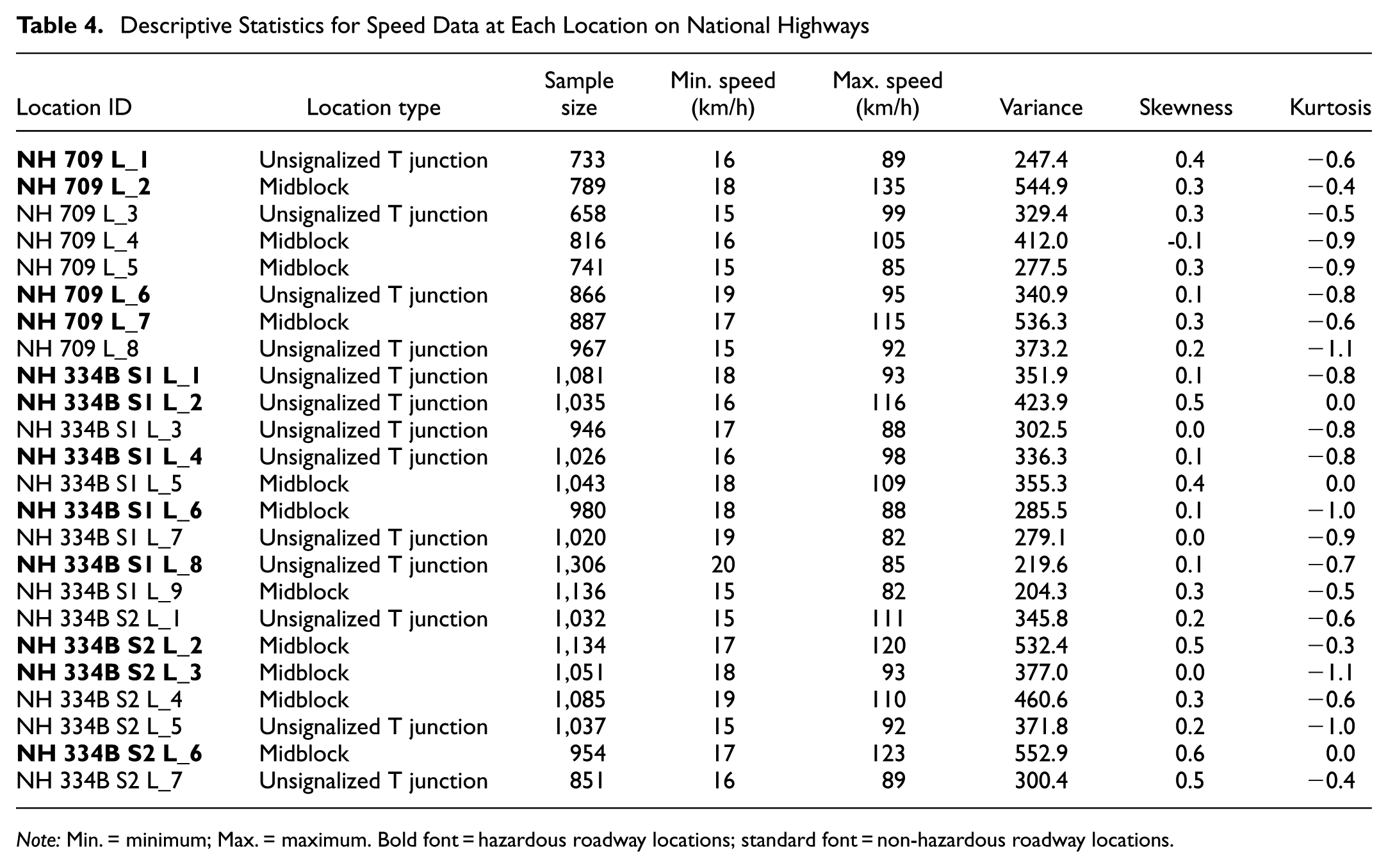
Note: Min. = minimum; Max. = maximum. Bold font = hazardous roadway locations; standard font = non-hazardous roadway locations.
Descriptive Statistics for Speed Data at Each Location on State Highways
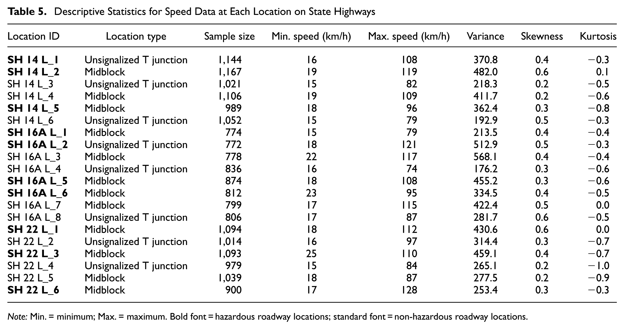
Note: Min. = minimum; Max. = maximum. Bold font = hazardous roadway locations; standard font = non-hazardous roadway locations.
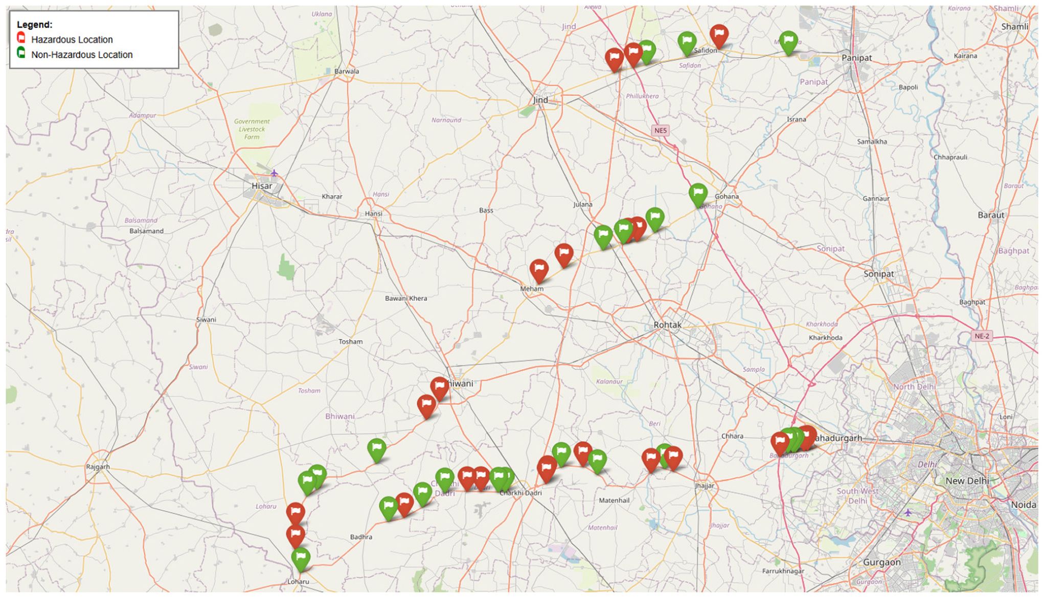
Spot speed data collection locations on National and State Highways.
The average sample size across all hazardous locations is relatively large, as given in Table 4, indicating sufficient data collection at each location. Extremely high speeds have been observed, from 82 to 135 km/h, while minimum speeds vary between 15 and 20 km/h. The variance in speed data shows significant variation across locations, from 204.3 to 552.9, indicating location-specific heterogeneity in vehicular traffic. Of note, midblock segments, such as NH 334B S1_L9 (non-hazardous) and NH 334B S2_L6 (hazardous), have the highest variances, indicating more dispersed speed profiles regardless of location type. For distributional shape, skewness values are predominantly between 0.1 and 0.6, indicating a slight right skew in speed distributions, which is common in mixed traffic conditions where a few high-speed vehicles increase the mean. The variance in speed data shows significant variation across locations, from 204.3 to 552.9, indicating location-specific heterogeneity in vehicular traffic.
The descriptive statistics for SH locations (Table 5) exhibit almost similar trends. HRLs have a minimum speed of 15 km/h and a maximum speed of 128 km/h.
Results
This section presents the results of fitting seven continuous probability distributions to spot speed data collected at hazardous and non-hazardous locations across six distinct highways. The subsequent results are analyzed using multiple interrelated criteria, such as KS test outcome, best-fit distribution, estimated parameters, mean speed with confidence intervals, data fraction variability, and repetition performance to determine whether the observed speeds significantly differ between HRLs and non-HRLs and how consistently the results remain stable across different data fractions and highways.
Distribution Trends of Observed Speed Data Across HRLs and Non-HRLs
The location, shape, and scale parameters of different parametric distribution models for vehicular speeds at specific HRLs and non-HRLs are presented in Tables A1 and A2 in the Appendix.
Based on penalized criteria, including Akaike Information Criterion (AIC) and BIC stands for Bayesian Information Criterion (BIC), as given in Tables A3 and A4 in the Appendix, the GEV distribution consistently provides the best-fit for spot speed data across all evaluated roadway segments under heterogeneous traffic conditions. Among the seven continuous probability distributions considered, the GEV outperformed the other distributions in capturing the underlying characteristics of speed variability. Therefore, all subsequent hypothesis testing evaluating significant differences in speed distributions between HRLs and non-HRLs will use the GEV distribution, given its superior GoF across diverse traffic contexts.
Distribution Robustness Across Data Fractions
The two-sample KS test evaluates whether the speed distributions at hazardous and non-hazardous locations are statistically different. As detailed in Table 6, unbold cells indicate that the test has rejected the null hypothesis (i.e.,
Two-Sample KS Test Statistics across Data Fractions and Repetitions (Rep) for Different Highways
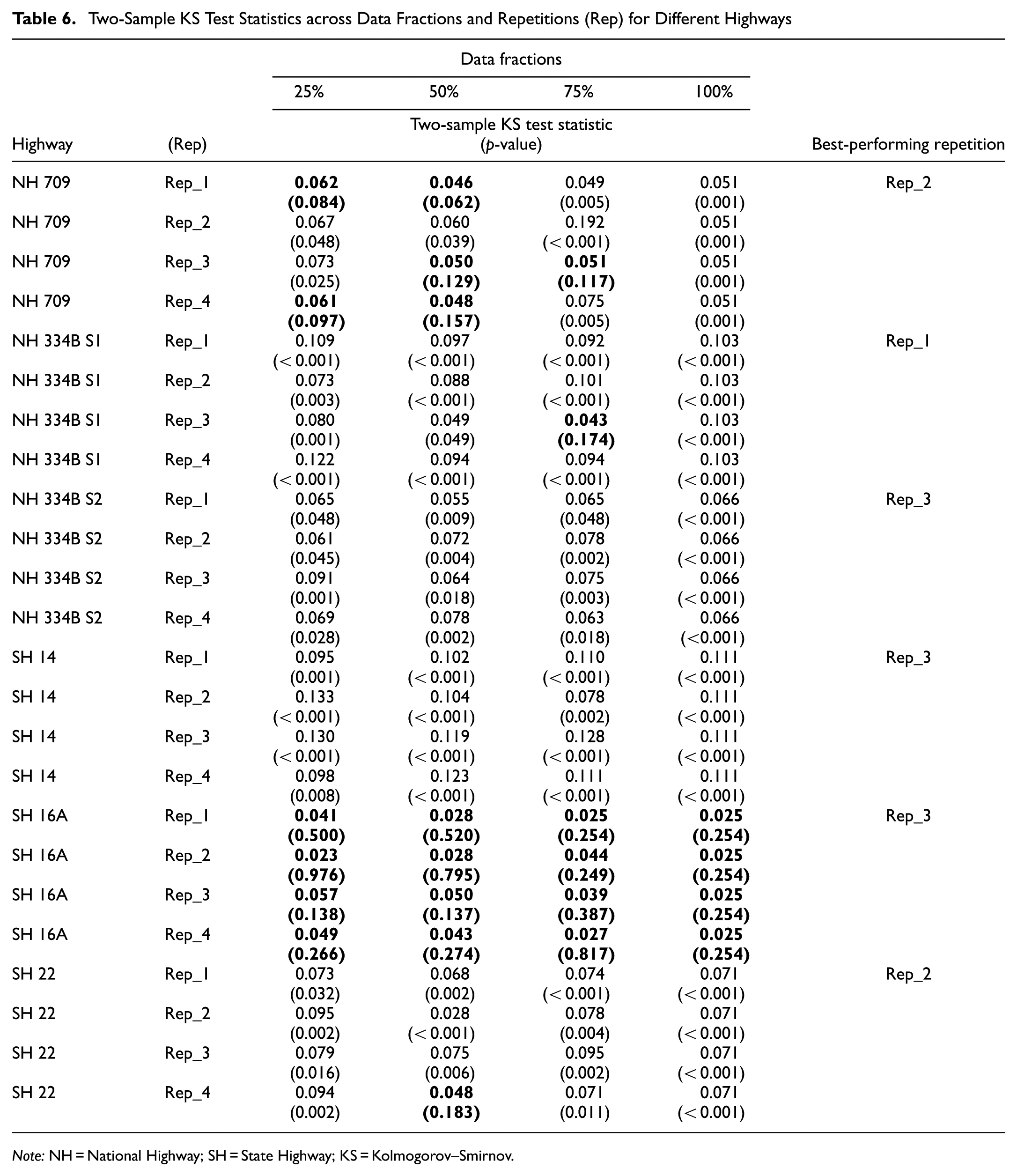
Note: NH = National Highway; SH = State Highway; KS = Kolmogorov–Smirnov.
An important finding from the two-sample KS testing is the consistent rejection of the null hypothesis across the majority of repetitions and data fractions, confirming that speed patterns differ statistically between HRLs and non-HRLs. The results, as mentioned previously, support the reliability of spot speed as a reliable indicator for evaluating roadway safety risk. An interesting pattern emerges while analyzing how the KS statistics and p-values vary across increasing data fractions (25%, 50%, 75%, 100%). The KS statistic values typically increase with data size across various highways (e.g., NH 709 and SH 14), suggesting that larger datasets improve the test’s ability to identify nuanced distributional differences ( 45 , 46 ). This pattern is simply because, as the percentage of available data or the sample size increases, the empirical estimates of the distribution parameters, such as shape, scale, and location, converge more closely to their true population values ( 47 , 48 ). Thus, the robustness of the fitted distributions improves with increased data fractions, thereby enhancing the reliability of the inference. However, in some cases (e.g., SH 16A), notably low KS statistics with high p-values have been observed across all data segments, potentially because of uniformity in driving behavior despite the nature of locations, resulting from local speed limits, lack of enforcement, and geometric consistency ( 49 , 50 ).
Sampling Repetitions and Model Robustness
In addition to distributional robustness, this study adopts a repetition-based framework to evaluate modeling consistency by creating four mutually exclusive datasets, or repetitions (Repetition_1–Repetition_4), for each highway and data fraction. The comparative analysis of repetitions (Table 6) shows that some repetitions consistently yield higher KS statistics and lower p-values across all data fractions, indicating a stronger ability to detect distributional differences between HRLs and non-HRLs. For example, Repetition_2 for NH 709, Repetition_1 for NH 334B S1, Repetition_3 for NH 334B S2, SH 14, SH 16A, and Repetition_2 for SH 22 have demonstrated consistent statistical significance (p < 0.05) and are thus deemed the most reliable. This consistency suggests that these datasets more accurately reflect the underlying distributional differences, possibly because of their better temporal coverage or a wider range of heterogeneity in traffic conditions ( 51 , 52 ). The implementation of repetition-based testing serves as a safeguard against overfitting to a particular data configuration and validates the robustness of the results across other observational environments ( 47 , 48 ). The study demonstrates that, even under varying real-world sample settings, the statistical differentiation between hazardous and non-hazardous locations remains consistently observable.
The comparative analysis of GEV distribution parameters, consisting of location, shape, and scale, between HRLs and non-HRLs across varying data fractions (25%, 50%, 75%, and 100%), as shown in Tables 7 and 8, provides significant insights into traffic speed characteristics for different highway types. The GEV location parameter consistently shows higher values for HRLs, indicating a greater tendency toward extreme-speed or crash risk in these segments than in non-hazardous roadway segments. For example, the location parameter for NH 709 ranges from 46.62 at the 25% data fraction to 45.51 at 100% data fraction at HRLs, whereas at non-HRLs, the values decrease from 45.14 to 44.37. Likewise, NH 334B S1 and S2 exhibit higher location parameters for HRLs, with NH 334B S1 achieving 46.73 at a 100% data fraction, compared to 42.84 for non-HRLs, indicating a distinct contrast between the two types of road segments. Similar trends have been observed across the majority of highways for vehicular speed profiles at hazardous and non-hazardous locations, particularly when speed deviations are pronounced but not extreme ( 52 , 53 ).
Parameter Estimates of Best-Fit Distribution across Data Fractions for Hazardous Locations
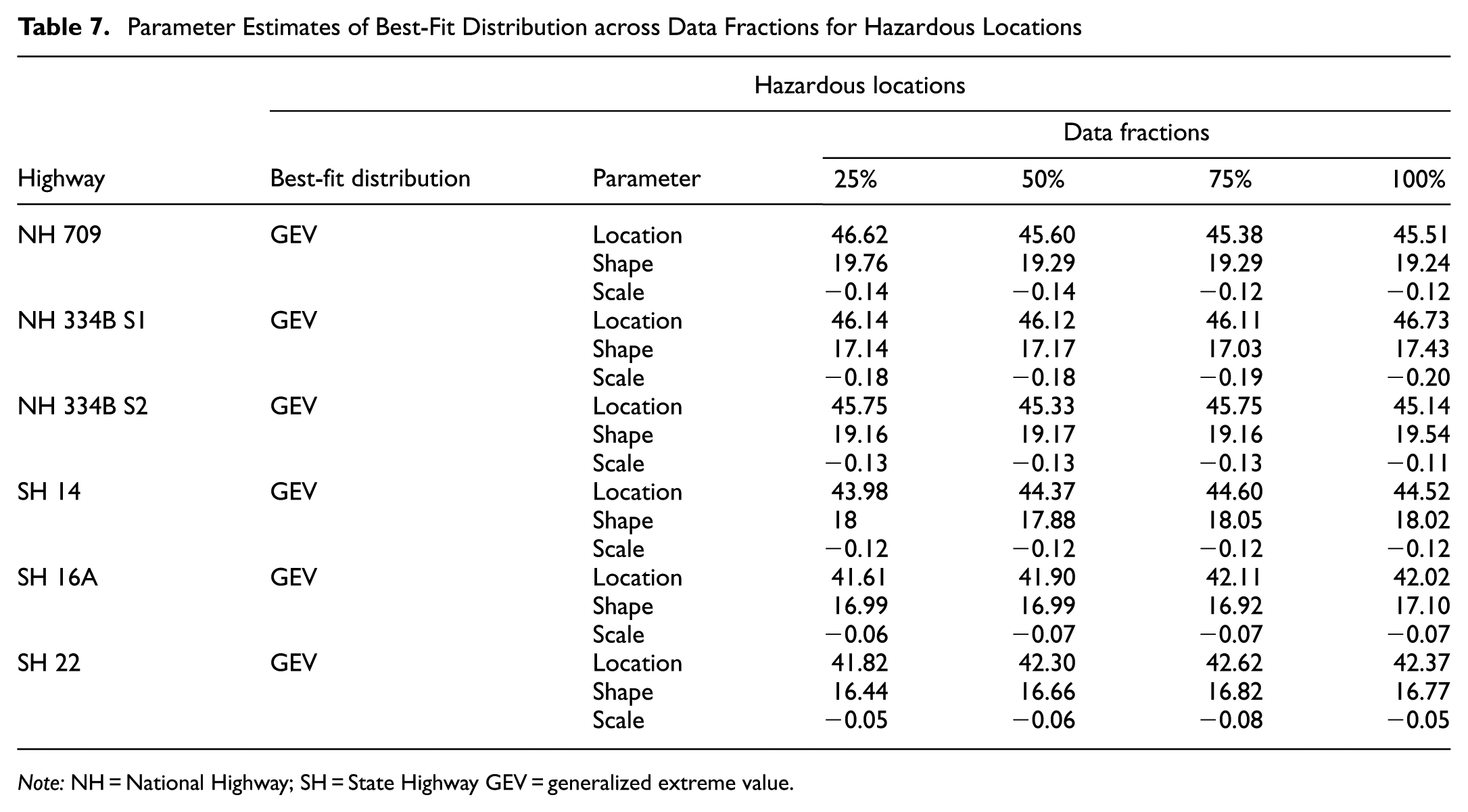
Note: NH = National Highway; SH = State Highway GEV = generalized extreme value.
Parameter Estimates of Best-Fit Distribution across Data Fractions for Non-Hazardous Locations
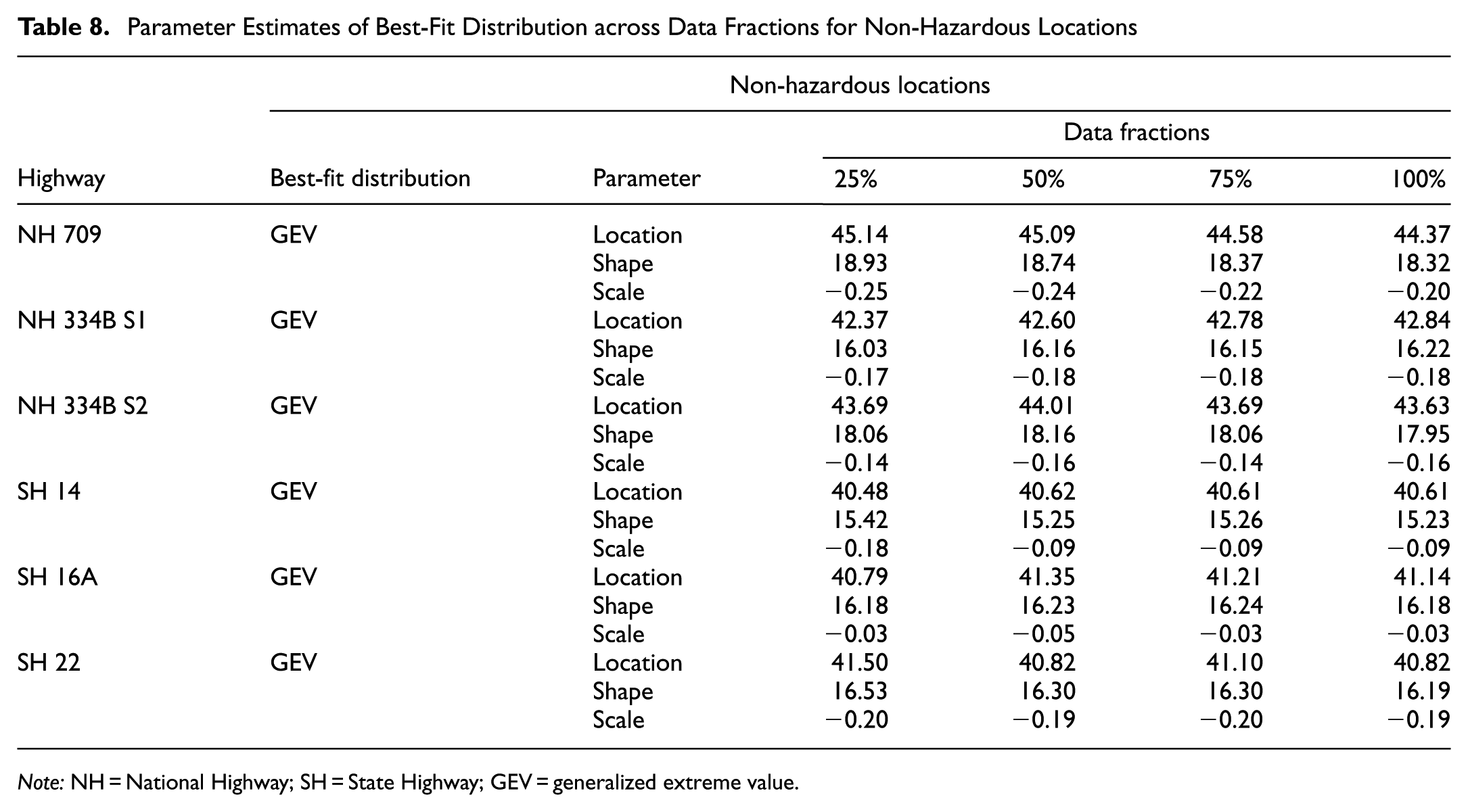
Note: NH = National Highway; SH = State Highway; GEV = generalized extreme value.
The shape parameters indicating the tail behavior of the distribution, the HRLs, often show higher values than non-HRLs, suggesting a greater frequency of crashes or speed events. For example, NH 709 has a shape parameter of 19.76 at the 25% data fraction for HRLs. In contrast, non-HRLs have a shape parameter of 18.93 and tend to exhibit lower values across data fractions. The shape parameter does not vary substantially across data fractions for HRLs and non-HRLs data, indicating a consistent distribution of extreme values within those segments. However, the non-HRLs demonstrate greater variability in the shape parameter. For example, in NH 334B S2, the shape parameter values vary from 18.06 at a 25% data fraction to 17.95 at 100% data fraction, suggesting a relatively less stable data distribution compared to HRLs ( 54 ). The scale parameter, which denotes the dispersion of the data, shows a consistent trend: HRLs exhibit less negative scale values than non-HRLs. For example, in NH 709, the scale parameter ranges from −0.14 to 0.12 for HRLs, whereas for non-HRLs it ranges from −0.25 to −0.20, further emphasizing the higher concentration of extreme values in hazardous zones.
Stability and Superiority of GEV Distribution Across Data Fractions
The cross-fractional analysis revealed significant consistency in identifying the best-fit distribution models. As shown in Tables 7 and 8, the GEV is the most stable and consistently best-performing model, both for HRLs and non-HRLs, and across nearly all highways and data fractions. Its flexibility in modeling skewed, tail-heavy vehicular speed distributions enhances its ability to fit empirical speed data. The GEV shape parameter k has marginally lower values at HRLs than at non-HRLs on the majority of highways, as shown in Tables 7 and 8, suggesting higher speed variability at locations associated with crash risk. The GEV is particularly sensitive due to its tail modeling capabilities ( 4 , 18 , 22 , 55 ). In these cases, three-parameter distributions, such as the Burr and GEV distributions, highlight the importance of capturing rare and high-magnitude deviations that are overlooked by two-parameter distributions, including the normal, gamma, and Weibull distributions ( 56 – 58 ). Importantly, as the sample size increases from 25% to 100%, the GEV distribution parameters consistently regain their statistical superiority across all highways, reaffirming the model’s parameter convergence and stability in larger data sets. This pattern aligns with statistical theory, which states that the asymptotic characteristics of estimators improve the fit quality and reduce estimation variance as the sample size increases ( 59 , 60 ). The consistent re-emergence of GEV as the best distribution in larger and more diversified data sets reinforces its methodological suitability and reliability for speed-based risk modeling ( 61 , 62 ).
The ECDFs and PDFs, along with fitted GEV distributions, collectively demonstrate the underlying distributional characteristics and tail behaviors of vehicle speeds between HRLs and non-HRLs along selected NHs and SHs, as shown in Figures 3 –8. Among these visualizations, CDFs illustrate shifts in overall speed levels by showing how rapidly the cumulative probability rises. In addition, PDFs highlight differences in dispersion and tail behavior, which are essential for understanding extreme-speed events on both HRLs and non-HRLs. The fitted GEV curves across all highways, including NH 709, NH 334B S1, NH 334B S2, SH 14, SH 16A, and SH 22, closely align with the empirical PDFs, especially in the upper-speed range, confirming their suitability for modeling the central and tail characteristics of observed speeds.
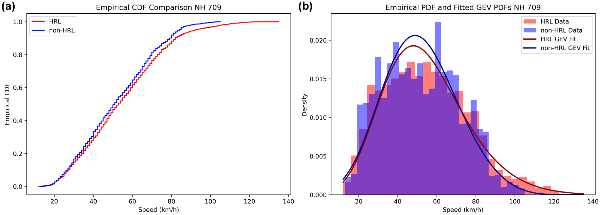
(a) Comparison of ECDFs and (b) PDFs with fitted GEV distributions for hazardous (HRL) and non-hazardous locations (non-HRLs) on NH 709.
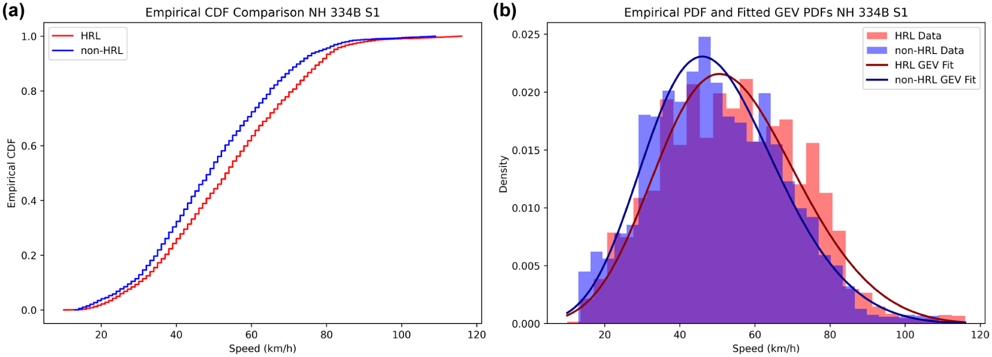
(a) Comparison of ECDFs and (b) PDFs with fitted GEV distributions for hazardous (HRL) and non-hazardous locations (non-HRLs) on NH 334B S1.
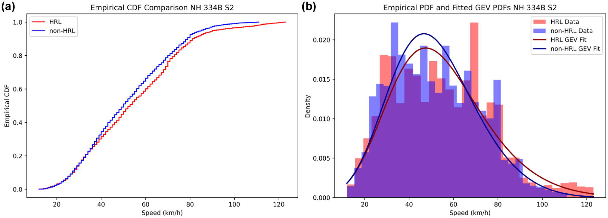
(a) Comparison of ECDFs and (b) PDFs with fitted GEV distributions for hazardous (HRL) and non-hazardous locations (non-HRLs) on NH 334B S2.
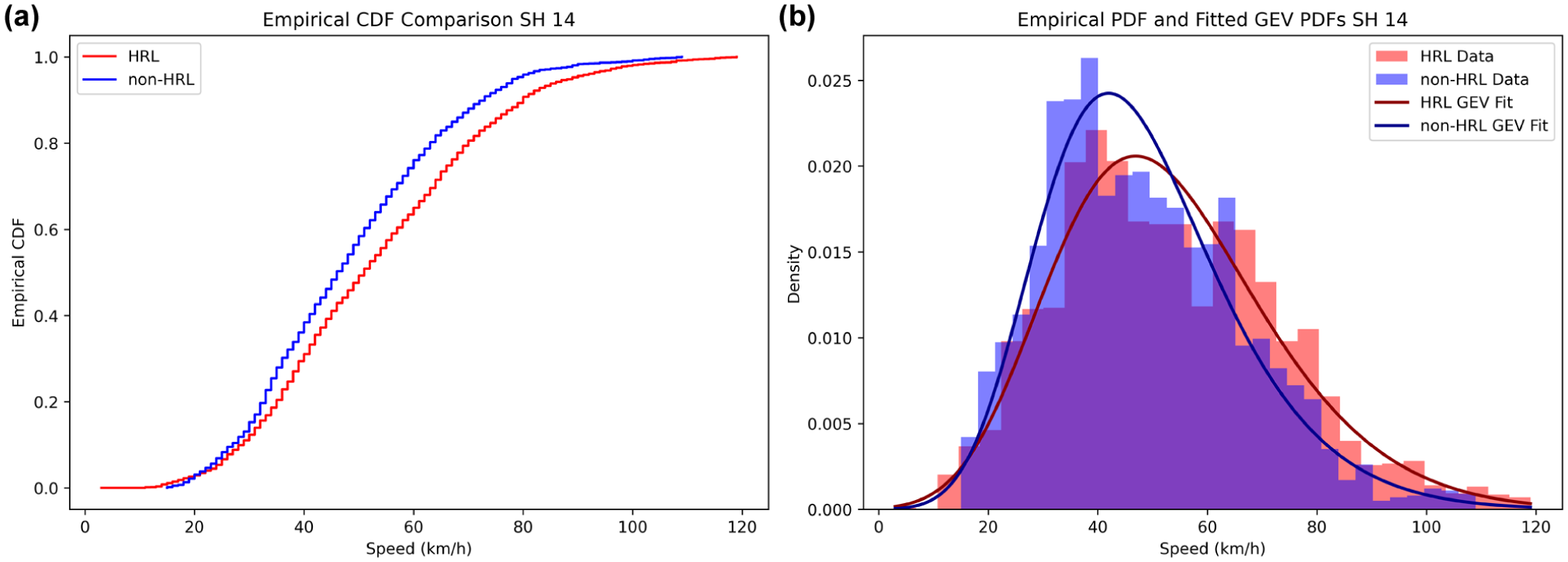
(a) Comparison of ECDFs and (b) PDFs with fitted GEV distributions for hazardous (HRL) and non-hazardous locations (non-HRLs) on SH 14.
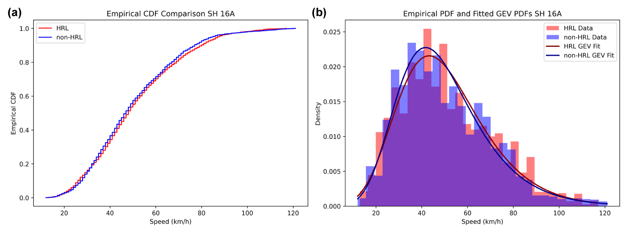
(a) Comparison of ECDFs and (b) PDFs with fitted GEV distributions for hazardous (HRL) and non-hazardous locations (non-HRLs) on SH 16A.
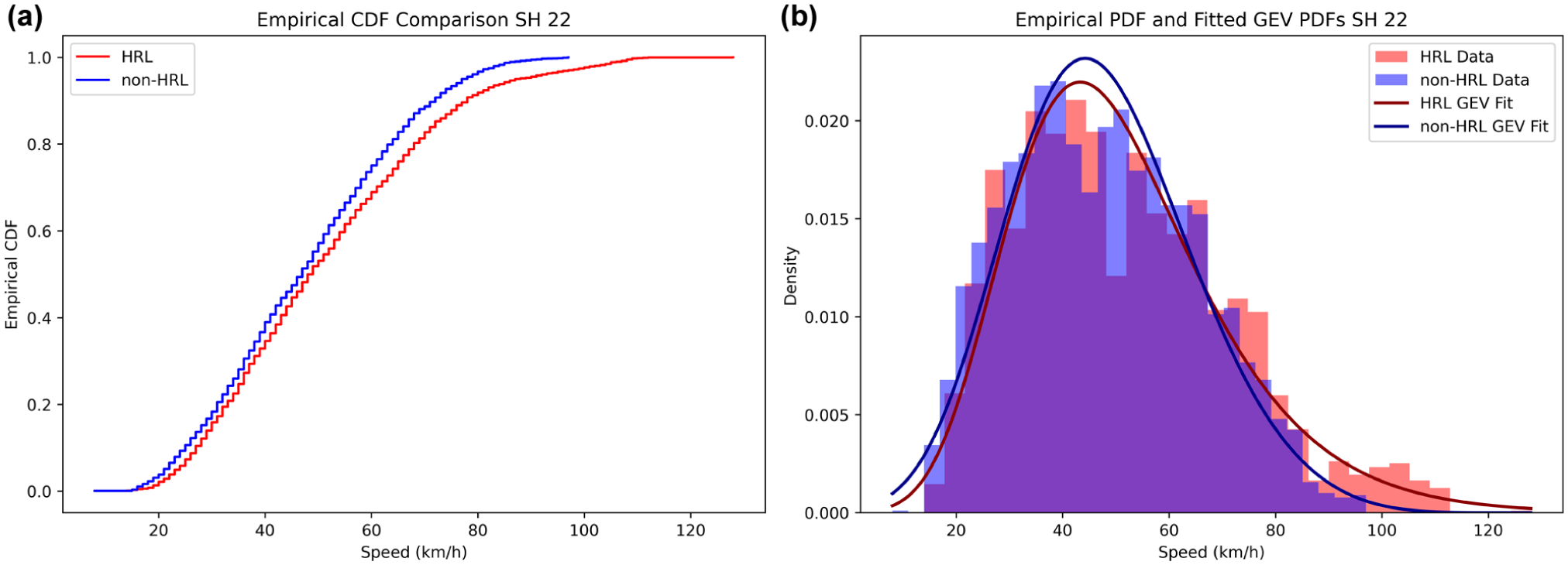
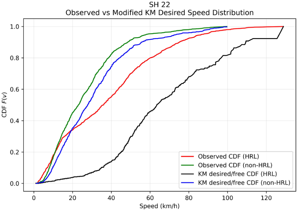
(a) Comparison of ECDFs and (b) PDFs with fitted GEV distributions for hazardous (HRL) and non-hazardous locations (non-HRLs) on SH 22.
On NHs, particularly NH 334B S1, as shown in Figure 4, the hazardous (hot spot) segment CDF is shifted to the right of the non-hazardous (non-hot spot) CDF over a significant portion of the mid-speed range, indicating consistently higher operating speeds at HRLs. This shift is characterized by a wider PDF with a heavier right tail, suggesting higher average speeds and increased speed variability and a greater likelihood of extreme-speed events. A related but more subtle pattern is observed on NH 334B S2 and NH 709, where the hazardous and non-hazardous CDFs largely overlap in the central region, implying similar typical speeds for the majority of drivers. However, separation becomes more evident in the upper-tail, as hazardous CDFs approach unity at higher speeds, and the corresponding PDFs exhibit extended right tails. This suggests that, on these highways, hazardous roadway differentiation is primarily influenced by a few, but significantly higher-speed, observations rather than a pronounced shift in average speed. The corresponding PDFs highlight this distinction, with HRLs exhibiting flatter peaks and heavier right tails, while non-HRLs have more sharply concentrated peaks around the modal speed range. In contrast, SH 22 shows a more moderately separated CDF for observed speeds at HRLs and non-HRLs, where differences between the two locations are less evident in the central region but become readily apparent in the upper-tail. The PDF comparison for SH 22 similarly shows greater dispersion and tail heaviness at HRLs, indicating that extreme-speed behavior plays a significant role in distinguishing risk-prone locations along this corridor.
SH 16A presents a different scenario in which the hazardous and non-hazardous CDFs and PDFs essentially coincide over most of the distribution. Both the central tendency and dispersion of speeds are comparable, indicating that the speed distribution alone has limited discriminatory power in distinguishing between HRLs and non-HRLs on this highway. This overlap suggests that factors other than speed, such as roadway geometric features, access density, traffic composition, and roadside population exposure, may be more influential in explaining crash occurrence on SH 16A, despite minor differences observed in the extreme tail of the GEV fits.
In summary, HRLs tend to exhibit broader distributions with heavier right tails, suggesting a higher likelihood of extreme-speed events. In contrast, non-HRLs show peaked distributions concentrated around the modal speed range, typically between 45 and 60 km/h. These distributional shapes are consistent with risk theory, which predicts that higher mean speeds and greater variability are associated with increased crash propensity.
Speed-Based Differentiation Between Hazardous and Non-Hazardous Locations
Table 9 presents a comparative analysis of mean vehicular speeds and their corresponding 95% confidence intervals across HRLs and non-HRLs for all highways under investigation. A systematic pattern is evident across almost all data fractions and highways, where HRLs consistently have higher mean speeds than non-HRLs. This pattern supports the hypothesis that high speeds are strongly associated with crash-prone locations, confirming speed as a major contributor to crash risk ( 63 – 66 ). The two-sample t-test confirms the statistical significance of speed differentials across HRLs and non-HRLs, with the majority of highways showing significant differences (p < 0.05) across all data fractions.
Comparison of Mean Speeds and Confidence Intervals (CIs) Across Data Fractions for Hazardous and Non-Hazardous Locations on Different Highways
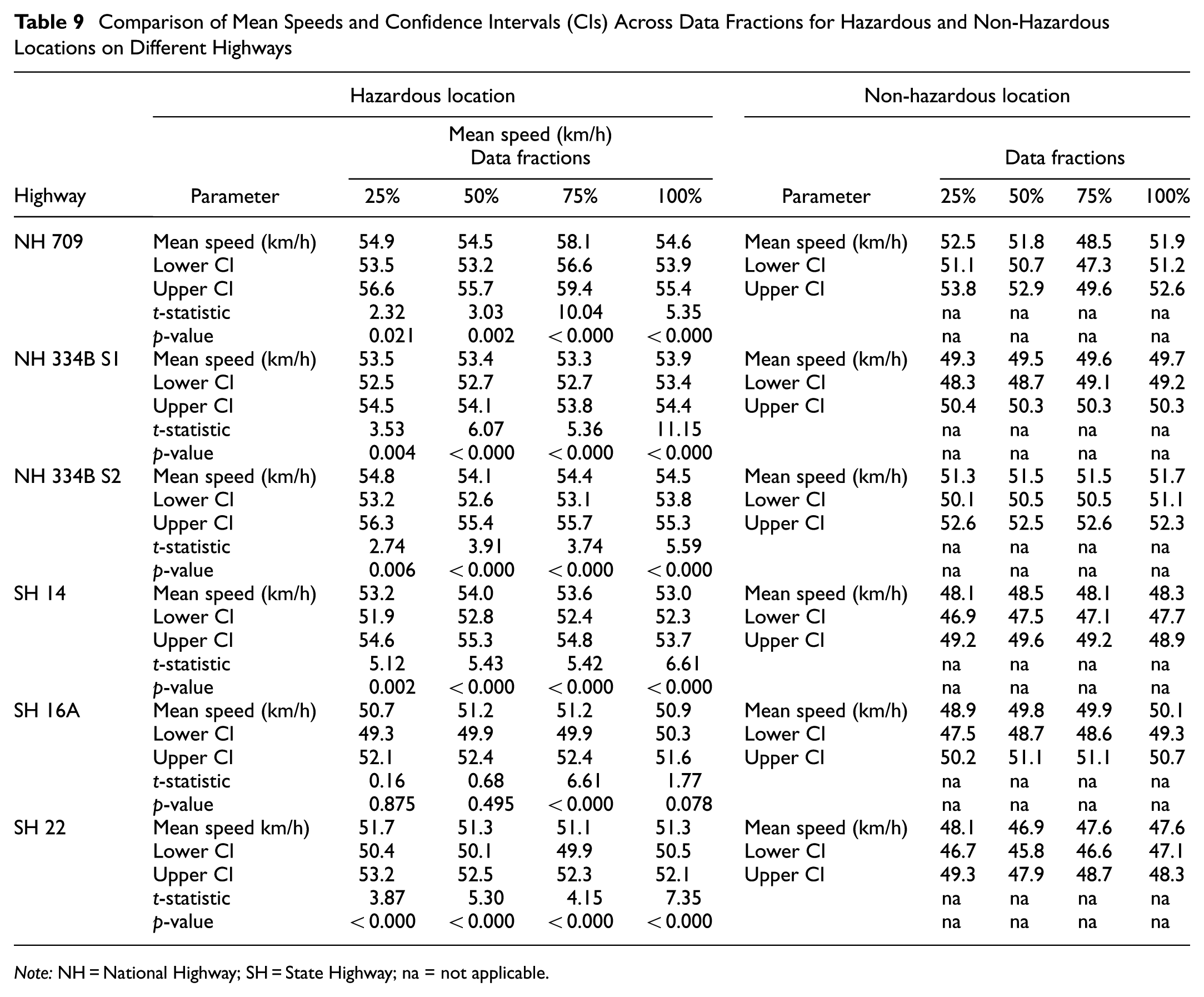
Note: NH = National Highway; SH = State Highway; na = not applicable.
Particularly higher statistics, such as those observed for NH 709 at the 75% fraction (t = 10.04), NH 334B S1 at the full data set (t = 11.15), and SH 22 across all data fractions (t range 3.87–7.35), provide strong evidence that the speed distributions at HRLs significantly differ from those at non-HRLs. These findings confirm that speed profiling is a reliable indicator of hazardous roadway environments.
Along with the overall consistency, some highways exhibit localized variations. For example, NH 709 exhibits an unusual increase in average speed at HRLs at the 75% data fraction. This localized variation may be because of context-specific anomalies, such as temporal changes in traffic composition or inconsistencies in speeding behavior over the data collection period ( 4 ). A similar consistency in trends has been observed in SH 14 and SH 22, where speeds at non-HRLs have remained relatively low, confirming the generalizability of speed-based risk differentiation ( 67 ). An exception occurs in SH 16A, where the speed differences between HRLs and non-HRLs are not significant at the 25% (t = 0.16, p = 0.875), 50% (t = 0.68, p = 0.495), and 100% (t = 1.77, p = 0.078) data fractions. This suggests that for SH 16A, speed may not be a strong predictor of road safety risk, implying that other contributing factors, such as geometric design inconsistencies, sight-distance constraints, driver behavior, road environment conditions, and vehicle malfunctioning, play a more significant role in shaping crash occurrence.
Congestion-Adjusted Desired Speed Analysis Using Modified KM-Based Speed Distribution
In this study, spot speed measurements have been collected during 2 h observation windows that may have experienced varying levels of traffic interaction. Differences in observed speeds between HRLs and non-HRLs could reflect temporary congestion rather than intrinsic speed behavior. To account for this possibility, a KM framework is used to estimate congestion-adjusted desired speed distributions. In this approach, time headways are first computed for each vehicle observation, and a site-specific headway threshold
Table 10 presents observed speed statistics and the congestion-adjusted desired speed estimates obtained using the modified KM framework, HRLs and non-HRLs across the analyzed highway corridors. The sample sizes n are from approximately 2,723 to 5,008 observations per location, providing a robust empirical basis for estimating the observed and the interaction-adjusted speed distributions. The mean observed speeds represent operating speeds influenced by vehicle interactions, and the modified KM desired speed
Comparison of Observed Speed Statistics and Kaplan–Meier (KM) Desired Speed Estimates for HRLs and non-HRLs
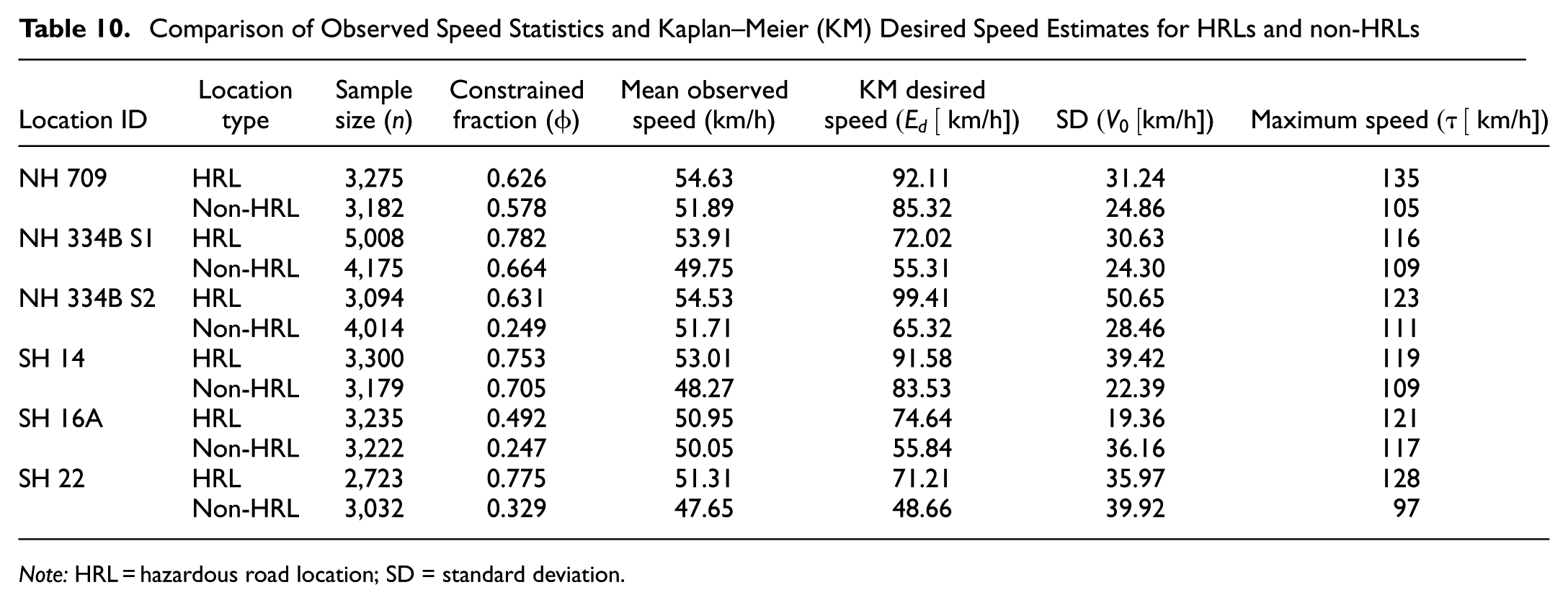
Note: HRL = hazardous road location; SD = standard deviation.
The constrained fraction
The distinction between interaction-influenced observed speeds and congestion-adjusted desired speeds is further illustrated by the CDFs shown in Figures 9 –14. The CDF plots illustrate the observed speed distributions along with the KM desired speed distributions for HRLs and non-HRLs across the six NH and SH corridors. In each figure, Figures 9 to 14 the red curve represents the observed speed CDF at HRLs, the green curve represents the observed speed CDF at non-HRLs, the black curve represents the KM estimated desired speed CDF for HRLs, and the blue curve represents the corresponding KM estimated desired speed CDF for non-HRLs. The observed curves reflect interaction-affected operating speeds, and the KM curves represent congestion-adjusted desired speed distributions, accounting for right-censored observations because of vehicle-following conditions. A comparison between the observed HRL and non-HRL curves shows that, across all six corridors, the HRL distributions are generally shifted toward higher speeds than the corresponding non-HRL distributions. This pattern is most evident on NH 334B S1, SH 14, and SH 22, where the red curves lie consistently to the right of the green curves over most of the central speed range, indicating that vehicles traversing hazardous segments often operate at higher speeds than those in non-hazardous locations. A similar pattern is observed across NH 709, NH 334B S2, and SH 16A, although with varying degrees of separation. These CDF representations are consistent with the observed mean speeds reported in Table 10, where HRLs exhibit higher operating speeds compared with non-HRLs across all six highways, with the largest observed differences on SH 14 (53.01 versus 48.27 km/h), NH 334B S1 (53.91 versus 49.75 km/h), and SH 22 (51.31 versus 47.65 km/h).
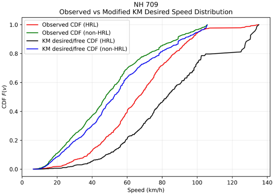
Comparison of observed speed CDFs for HRLs and non-HRLs with the modified KM estimated desired speed distribution for NH 709.
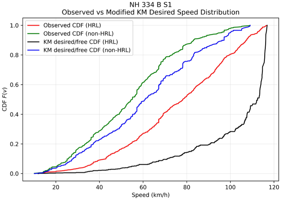
Comparison of observed speed CDFs for HRLs and non-HRLs with the modified KM estimated desired speed distribution for NH 334B S1.
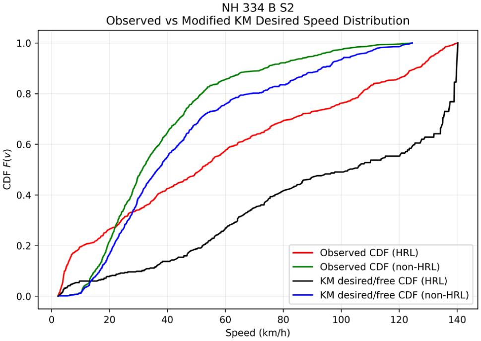
Comparison of observed speed CDFs for HRLs and non-HRLs with the modified KM estimated desired speed distribution for NH 334B S2.
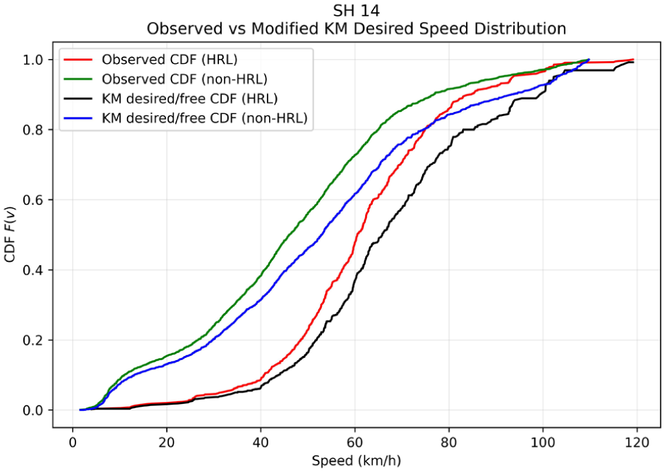
Comparison of observed speed CDFs for HRLs and non-HRLs with the modified KM estimated desired speed distribution for SH 14.
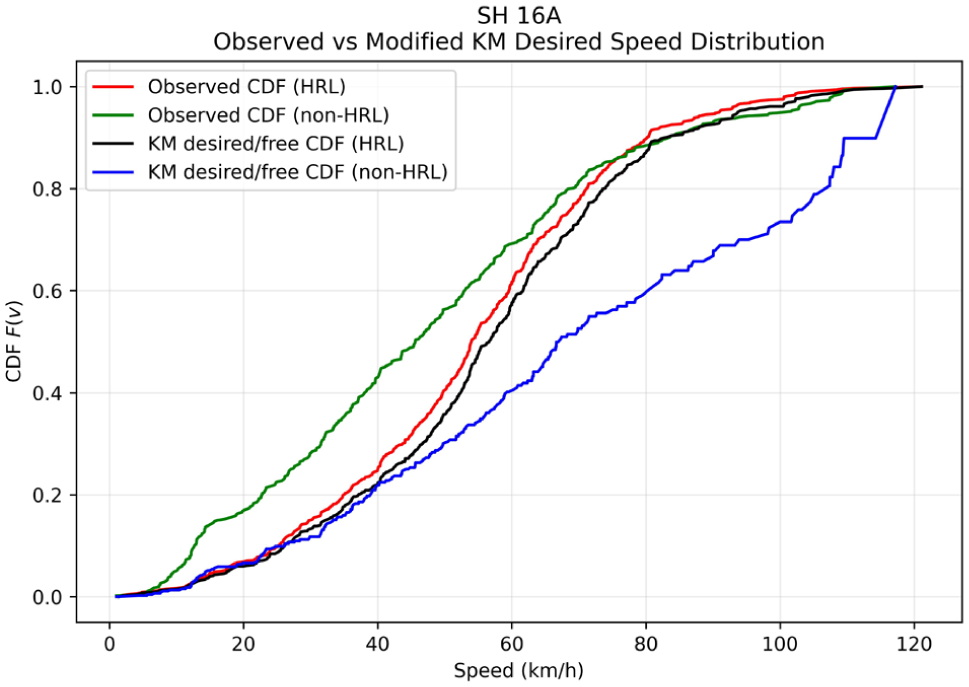
Comparison of observed speed CDFs for HRLs and non-HRLs with the modified KM estimated desired speed distribution for SH 16A.
Comparison of observed speed CDFs for HRLs and non-HRLs with the modified KM estimated desired speed distribution for SH 22.
The intra-location comparison between observed and KM curves further highlights the effect of traffic interaction on observed speeds. In all corridors, the KM desired speed curves are shifted to the right of the corresponding observed curves, indicating that the desired speed distribution is higher than the directly observed operating-speed distribution once vehicle-following effects are accounted for. The pattern is apparent in the HRL curves for NH 334B S1, NH 334B S2, SH 14, and SH 22, where the significant deviation between the red and black curves indicates a substantial suppression of observed speeds because of traffic interaction. A comparable but generally smaller separation is visible between the green and blue curves for non-HRLs. These CDF placements are consistent with the numerical differences between the mean observed speed and the KM desired speed listed in Table 10. For example, on NH 334B S2, the observed mean speed is 54.53 km/h, while the KM desired speed is 99.41 km/h; similarly, on SH 14, the observed mean speed is 53.01 km/h, whereas the KM desired speed is 91.58 km/h. This suggests that field-observed spot speeds underestimate the underlying desired speed potential when vehicle-following effects are present.
The most important comparison, however, is between the KM-adjusted HRL and non-HRL curves, because this directly tests whether the speed differences persist after accounting for congestion and platooning effects. Across all six corridors, the KM HRL curve (black) is predominantly shifted to the right of the KM non-HRL curve (blue), indicating that hazardous locations have a higher desired speed distribution even after interaction-induced suppression is accounted for. This is particularly evident on NH 334B S1, NH 334B S2, SH 14, SH 16A, and SH 22, where the black curve consistently maintains a superior speed position compared with the blue curve for the majority of the distribution. The corridor-specific differences in separation magnitude suggest that the extent to which hazardous locations differ from non-hazardous locations is not uniform across corridors; however, the overall pattern remains consistent: HRLs generally exhibit higher desired speed potential than non-HRLs. This indicates that the observed speed differences between HRLs and non-HRLs cannot be attributed solely to variations in instantaneous traffic density during the measurement windows, but rather reflect intrinsic roadway and behavioral characteristics, including longer uninterrupted tangents, higher perceived design speeds, or delayed speed adaptation near intersections, roadside minor accesses, fuel stations, and merging and diverging sections.
In conclusion, the observed speed statistics, the KM desired speed estimates, and the corresponding CDF visualizations provide a consistent understanding of speeding behavior across roadway segments. The mean observed speeds reflect operational conditions influenced by interactions, and the KM-based desired speeds isolate the intrinsic desired speed potential by including right-censored observations because of vehicle-following. The CDF plots further confirm that the speed distributions at HRLs systematically extend into higher-speed ranges than those at non-HRLs. This indicates that higher operating speeds and a greater likelihood of extreme-speed events characterize hazardous segments. These patterns align with well-established road safety theory, which links higher desired speeds and greater speed variability to higher crash risk ( 33 , 34 ). Therefore, the combined evidence suggests that the increased speeds observed near HRLs reflect intrinsic speed-selection behavior linked to roadway characteristics rather than solely variations in traffic density.
Discussion
This study investigates the statistical dynamics of vehicular spot speeds at identified HRLs and non-HRLs across six NH and SH corridors using a multi-stage data fractionation (i.e., at 25%, 50%, 75%, and 100%) and a multi-layered analytical framework. The framework combines continuous probability distribution modeling, inferential statistical testing, and congestion-adjusted desired speed estimation. This study aims to examine if there is a statistically significant difference in speed behavior between identified HRLs and non-HRLs on rural two-lane highways under mixed traffic conditions.
The distribution fitting results demonstrate that the GEV distribution consistently provides the best statistical representation of the observed spot speed data across all highways and sampling fractions. The GEV model’s superiority is supported by penalized fit criteria such as AIC and BIC, and subsequently reflects the GEV’s ability to capture skewness, heavy tails, and high-speed extremes. These characteristics are commonly observed in mixed traffic environments with weak lane discipline and frequent overtaking behavior ( 68 ). Furthermore, as the sample fractions increased, GEV parameter estimates showed consistent convergence, indicating reduced estimation variance and improved reliability, a pattern consistent with conventional asymptotic characteristics. The heavy-tail sensitivity of the GEV distribution is particularly useful for capturing rare but critical extreme-speed events that often contribute disproportionately to crash risk ( 4 ). GEV-based modeling enhances the diagnostic capacity of speed-based safety assessments by accurately modeling both central and extreme behavior ( 16 , 18 , 23 ).
The comparative analysis of speed distribution using the KS test provides strong evidence that the distributional form of speeds differs significantly between HRLs and non-HRLs on the majority of highways. Significant KS test outcomes across major highways indicate that HRLs exhibit higher speeds and higher variability and heavier right-tailed characteristics, which are often associated with increased crash potential ( 69 , 70 ). These distributional characteristics were graphically supported by empirical CDF and PDF plots, which showed HRLs with flatter, right-shifted CDFs and broader PDFs, indicating higher variability and a higher likelihood of extreme-speed events. These characteristics align with established risk theory, which implies that crash likelihood increases in environments where the average speeds and variability surpass typical operating conditions ( 64 ). The stability of the KS test results across multiple sampling repetitions further strengthens the conclusion that speed behavior systematically differs across risk categories. This study confirmed that distributional differences were not dependent on any specific data configuration, as analyzed using four mutually independent repetitions for each highway and sample fraction. The consistent statistical significance observed across several highways in different repetitions indicates robustness to temporal fluctuations, traffic heterogeneity, and sampling variability ( 44 , 52 , 71 , 72 ). Repetitions that consistently yielded significant results presumably captured broader traffic conditions characterized by more pronounced behavioral heterogeneity, providing a stronger differential capability. This methodological design, focused on repetition-based validation, provides an additional buffer against overfitting or misinterpretation arising from single-sample analyses, a common shortcoming in earlier road traffic speed-safety research ( 73 ).
In addition to distributional assessments, the comparison of mean speeds between HRLs and non-HRLs revealed a consistent and significant pattern, where hazardous locations consistently exhibit higher mean speeds across almost all data fractions and highways. The two-sample t-tests validate the statistical significance of these differences, with several highways, such as NH 709, NH 334B S1, and SH 22, exhibiting notably high t-statistics, indicating substantial divergence in central tendencies ( 74 , 75 ). These findings provide empirical support for the long-standing understanding that high speed remains a principal determinant of crash likelihood and crash severity ( 76 , 77 ). However, the joint consideration of KS and the t-test results highlights subtle differences. The majority of highways showed good alignment between the two tests, while certain corridors, such as SH 16A, showed significant differences between the two tests. This discrepancy suggests that speed behavior alone does not adequately explain the potential crash risk in these locations, implying the influence of geometric design factors, road environment conditions, vehicle conditions, traffic volume, and road user behavior ( 78 , 79 ). However, NH 709 showed cases where the t-test was significant, while the KS test was not, highlighting situations in which mean speeds differ despite similar distributional shapes. These discrepancies align with theoretical expectations: t-tests capture differences in central tendency, and the KS test reveals a shift in the overall distribution. These findings highlight the significance of using both statistical measures to capture complementary dimensions of speed behavior.
Given the underlying roadway environment and traffic characteristics, the observed speed across identified HRLs and non-HRLs during short-term measurements is more likely to reflect transient congestion than intrinsic speed behavior. Vehicles that operate in platoons or under the car-following conditions may experience speed suppression because of preceding vehicles, which can obscure drivers’ intrinsic speed-choice behavior. To address this issue, this study incorporates the KM framework to estimate congestion-adjusted desired speed distributions. In this approach, vehicles traveling under interaction conditions are treated as right-censored observations and unconstrained vehicles are treated as uncensored observations. The comparison of mean observed speeds with KM estimated desired speeds reveals that traffic interactions substantially suppress the observed speed distributions in HRLs and non-HRLs. In several corridors, the KM-derived desired speed estimates significantly surpassed the corresponding observed mean speeds, indicating that interaction effects over the observation period influence the measured spot speeds. However, the KM-based results also show that HRLs generally maintain higher desired speeds and exhibit broader upper-tail speed characteristics, even after accounting for these interaction effects. This finding suggests that the higher-speed behavior observed at hazardous locations cannot be attributed solely to temporary variations in traffic density during the observation period. Instead, it reflects intrinsic roadway characteristics and behavioral responses associated with hazardous roadway environments. The KM-based CDFs further illustrate the distinction between interaction-influenced operating speeds and the desired speed. In the majority of corridors, the desired speed CDF lies to the right of the observed speed CDFs, confirming that the KM approach effectively reconstructs the suppressed portion of the speed distribution. Furthermore, HRL distributions frequently exhibit greater dispersion and more pronounced upper-tail characteristics than non-HRL segments, reinforcing the notion that hazardous segments correlate with higher speed potential and more heterogeneous driver behavior.
The combined evidence from distribution modeling, inferential testing, and KM-based desired speed analysis provides a comprehensive characterization of speed behavior across hazardous and non-hazardous roadway environments. Hazardous locations are characterized by higher mean speeds and broader dispersion, heavier upper tails, and higher desired speed potential. These characteristics indicate that hazardous segments allow or encourage speed choices that are inconsistent with the surrounding roadway environment or conflict density. Therefore, this study’s results validate the adopted methodological design comprising repeated subsampling, KS and t-test comparisons, and continuous probability distribution fitting, and KM-based desired speed distributions as a robust framework for analyzing road user speeding behavior in hazardous and non-hazardous roadway environments under heterogeneous traffic conditions.
From a traffic management perspective, these findings indicate that uniform corridor-level speed limits are insufficient to address localized risk mechanisms ( 80 , 81 ). Speed management strategies should be driven by distribution-based diagnostics, especially those capturing upper-tail behavior. Previous studies indicate that crashes on rural highways are disproportionately associated with speed variance and extreme speeds rather than mean speeds alone ( 33 , 82 , 83 ). Therefore, the fitted GEV parameters and percentile-based speed thresholds derived from HRLs can be used to identify locations where a small proportion of high-speed vehicles substantially increase crash risk ( 84 ). Given the crash history on these NHs and SHs, the HRLs are concentrated near roadside eateries, fuel stations, minor access points, and culverts, where merging and diverging movements interact directly with uninterrupted through traffic.
The findings support the implementation of location-specific speed transition strategies before access-dense sections. Empirical evidence from rural highway studies suggests that gradual speed reduction zones, supported by advance warning signs and perceptual speed reduction measures, are more effective than sudden speed limit changes ( 85 , 86 ). Distributional speed analysis can suggest the placement and length of these transition zones by identifying the distance at which upper-tail speeds start to deviate from non-hazardous patterns ( 87 – 89 ). This approach correlates speed control with observed driving behavior rather than relying solely on prescriptive geometric standards.
The heavy-tailed speed distributions observed at hazardous segments also provide a strong empirical justification for targeted speed enforcement strategies. Rather than enforcing compliance uniformly across all vehicles, enforcement efforts can be concentrated on the upper-tail of the speed distribution where marginal reductions provide the most significant safety benefits ( 90 , 91 ). Automated speed enforcement, mobile enforcement units, or dynamic speed feedback displays can be strategically placed before approaching an identified hazardous location, prioritized using GEV-based exceedance probability. Data-driven and targeted interventions should be widely accepted among road users to significantly improve enforcement efficiency, particularly in resource-constrained rural areas ( 92 , 93 ).
Conclusions
This study aims to examine whether there is a statistically significant difference in speed behavior between identified HRLs and non-HRLs on rural two-lane highways under mixed traffic conditions. The HRLs and non-HRLs were systematically identified using an NB-L model and a KDEB approach, based on police-reported, georeferenced crash data obtained from the State Police CCTNS for 2017–2019. This study uses an integrated analytical framework that incorporates two-sample KS tests, t-tests, and seven continuous probability distributions to model spot speeds. Seven continuous probability distribution functions, including the normal, lognormal, gamma, logistic, Weibull, Burr, and GEV distributions, were applied to determine the best-fitting distributions for distinct locations on NHs and SHs. KS tests, as well as t-tests, are used to determine statistically significant differences in spot speeds across HRLs and non-HRLs, utilizing a multifractional data and repetition design framework. This study treats each measurement site as an independent observational unit, maintains a constant observation duration, and focuses on location-specific speed behavior rather than the effects of spatial or temporal coverage. The combination of GoF metrics (AIC and BIC), distributional parameter estimates (location, scale, and shape), and inferential testing (two-sample KS) has allowed for a statistically robust and empirically validated evaluation of speed behavior concerning road safety.
In addition, the modified KM analysis is used to distinguish the desired speeds from the observed speeds, accounting for the effects of traffic density and congestion. The KM technique facilitates the reconstruction of the underlying desired speed distribution for each location by differentiating between unconstrained and interaction-constrained observations using headway-based censoring. The resulting desired speed estimates showed that, even after accounting for vehicle-following effects, HRLs generally maintain higher desired speed potential, greater speed dispersion, and stronger upper-tail speed behavior than non-HRLs. This confirms that the higher-speed characteristics at hazardous segments cannot be attributed solely to differences in instantaneous traffic density during the observation period but are also associated with roadway characteristics and behavioral factors.
This study provides statistically stable and practically relevant insights on speed-related risk differences between HRLs and non-HRLs. The results demonstrate that the GEV distribution consistently outperforms other distributions in HRLs and non-HRLs, highlighting its empirical adaptability and suitability for modeling spot speed data and capturing extreme tail behavior in heterogeneous traffic conditions, where standard normality assumptions for vehicular speed data may be invalidated. The comparative findings across various data fractions indicate that larger data sizes improve model reliability, parameter stability, and inferential robustness, underscoring the statistical benefits of larger sample sizes in transportation safety research. Furthermore, the KS test findings indicate that spot speeds significantly differ across HRLs and non-HRLs on the majority of highways, with HRLs exhibiting higher speeds, higher variability and heavier right-tailed characteristics, which are often associated with increased crash risk. The stability of the KS test results across multiple sampling repetitions further strengthens the notion that speed behavior varies substantially between HRLs and non-HRLs. The combined results from the KS test, t-test, and GEV model indicate that speed behavior, characterized by distributional shape, central tendency, variability, and tail behavior, serves as a robust, statistically validated criterion for distinguishing the associated risk between HRLs and non-HRLs.
This study demonstrates speed distribution analysis, extending beyond simple descriptive characterization to facilitate targeted, data-driven safety interventions on rural two-lane highways. The findings indicate that HRLs are more consistently characterized by increased dispersion and a propensity for extreme speeds than by uniformly higher mean speeds, particularly in areas with frequent roadside access and complex merging and diverging conditions. For safety management, the findings support a shift toward segment-specific speed management strategies that prioritize locations exhibiting heavy-tailed speed distribution, especially near eateries, fuel stations, minor access roads, and culverts. Distribution-informed interventions, such as graduated speed transition zones, upper-tail-focused enforcement, and context-sensitive speed feedback systems, offer a scalable, evidence-based approach to reduce crash risk in heterogeneous traffic environments. By explicitly linking speed distribution characteristics to roadway environment and access-related risk mechanisms, the proposed framework provides a realistic decision-support tool for improving safety on rural undivided highways.
Despite its empirical rigor, this study has certain limitations. This study exclusively focused on traffic speed analysis as a univariate distributional analysis, failing to capture the full range of dynamics that affect the road user’s risk level, speeding behavior, and crash likelihood, which is influenced by traffic flow, geometric design characteristics, meteorological conditions, lighting, enforcement intensity, and driver gender and age composition. Therefore, future studies may extend the spot speed analysis to include multilane highways and integrate the aforementioned factors that influence crash risk, speeding behavior, and crash propensity, using a multivariate modeling approach to achieve a more comprehensive understanding of speed-risk relationships. A longitudinal approach that considers temporal variations in speeding behavior during day and night, peak and off-peak periods, and seasonal variations such as summer, winter, and rainy seasons may uncover dynamic patterns that are frequently overlooked in static analyses. The observed stabilization of distributional estimates after approximately three-fourths of the full data provides empirical insight for conducting efficient spot speed analysis underlying traffic and roadway environments. Further studies may focus on determining universal minimum sample size thresholds, using longer monitoring periods and continuous data sources to improve model robustness.
Supplemental Material
sj-docx-1-trr-10.1177_03611981261448538 – Supplemental material for Evaluating the Reliability and Consistency of Statistical Models for Speed Distribution Analysis at Hazardous and Non-Hazardous Roadway Locations: Multifraction Data Set Approach
Supplemental material, sj-docx-1-trr-10.1177_03611981261448538 for Evaluating the Reliability and Consistency of Statistical Models for Speed Distribution Analysis at Hazardous and Non-Hazardous Roadway Locations: Multifraction Data Set Approach by Parveen Kumar, Geetam Tiwari and Sourabh Bikas Paul in Transportation Research Record
Footnotes
Acknowledgements
We would like to extend our gratitude to all faculty members and researchers who have provided invaluable support throughout our research work. We would also like to express our gratitude to Parvinder Ghanghas for his help with data collection through the site surveys.
Author Contributions
The authors confirm contribution to the paper as follows: study conception and design: Parveen Kumar; data collection: Parveen Kumar; analysis and interpretation of results: Parveen Kumar, Geetam Tiwari, and Sourabh Bikas Paul; draft manuscript preparation: Parveen Kumar, Geetam Tiwari, and Sourabh Bikas Paul. All authors reviewed the results and approved the final version of the manuscript.
Declaration of Conflicting Interests
The authors declared no potential conflicts of interest with respect to the research, authorship, and/or publication of this article.
Funding
The authors disclosed receipt of the following financial support for the research, authorship, and/or publication of this article: The authors acknowledge the research fellowship from the Ministry of Housing and Urban Affairs, (MoHUA), erstwhile the Ministry of Urban Development (MoUD), the Government of India (IITD/TRIPP/MUL/2023-2024/25436).
Data Accessibility Statement
The data will be available on reasonable request.
Supplementary Material
Supplemental material for this article is available online.
References
Supplementary Material
Please find the following supplemental material available below.
For Open Access articles published under a Creative Commons License, all supplemental material carries the same license as the article it is associated with.
For non-Open Access articles published, all supplemental material carries a non-exclusive license, and permission requests for re-use of supplemental material or any part of supplemental material shall be sent directly to the copyright owner as specified in the copyright notice associated with the article.