
Abstract
Cycle-level delay estimation plays an important role in the performance evaluation for dynamic signal control at intersections. With the popularity of connected vehicles (CVs), CV trajectory data have been investigated in delay estimation. However, CV trajectory-based studies mainly focus on fixed-time signal control, with low CV penetration rates remaining a challenge for dynamic signal control. This study proposes a cycle-by-cycle delay estimation method using CV trajectory data at an isolated intersection with dynamic signal control in undersaturated conditions. Historical CV trajectories within the same time-of-day period across days are transformed into Newellian coordinates and then aggregated to cope with low penetration rates. Vehicle arrival distribution under a Bernoulli process is estimated. The evolution of the queued vehicle number within each cycle is analytically modeled using the stochastic point-queue model. A probabilistic delay estimation model is built for cycle-level delay estimation, making full use of observed trajectory data. To cope with computational burden, the evolution of queued vehicles’ arrival in the red time is approximated based on the deterministic point-queue model. The simulation experiments validate the advantages of the proposed model over benchmarks for estimation accuracy and error variance. The performance of the proposed model remains relatively stable even with low CV penetration rates. The sensitivity analyses show that the proposed model is robust to penetration estimation errors, traffic demand levels, and arrival patterns with undersaturated traffic.
Introduction
Urban traffic congestion is a major challenge for transportation efficiency. As key road network nodes, intersections often become bottlenecks and cause a large share of overall delays. Signalized intersections account for 34% of total urban delay, approximately 295 million vehicle hours of annual delay in US urban areas ( 1 ), resulting in substantial societal and economic losses. To reduce intersection delays under stochastic and time-varying demand, dynamic signal control is widely used. Cycle-level delay estimation plays an important role in the performance evaluation for dynamic signal control at intersections.
Traditional methods for estimating delays at signalized intersections primarily rely on data collected by fixed-point detectors (e.g., loop detectors, geomagnetic sensors, cameras, and Radio Frequency Identification (RFID)). Its method has evolved through three stages ( 2 ): (1) 1920s–1970s, which focused on steady state theory, of note, Webster’s 1958 stochastic model for average control delay with Poisson-distributed arrivals ( 3 ); (2) 1970s–2000s, where dynamic models emerged using coordinate transformation, incorporating upstream intersection effects. The 1994 Highway Capacity Manual (HCM) revised its formula for coordinated arterial intersections, gaining recognition as a reliable method (2); and (3) 2000s onwards, where improved approaches appeared, including HCM-based models for varying saturation ( 4 ), multiple linear regression models ( 5 ), simulation-based neural networks ( 6 ), and kinematic equation-derived linear models for individual vehicle delay ( 7 ). However, because of limited coverage, high installation and maintenance costs, and vulnerability to damage of fixed-point detectors, delay estimation methods based on these detectors have significant limitations.
Recent years have seen rapid advances in connected vehicles (CVs), mobile internet, and vehicle–infrastructure integration, driving widespread adoption of connected taxis and mobility services (e.g., Baidu Maps). High-precision, high-sampling-frequency CV trajectory data has become a critical traffic control data source. In-depth mining of this data captures intersection vehicle states more accurately, offering advantages over fixed detectors, broader coverage and larger volumes, supporting innovative intersection delay estimation methodologies. These studies mainly fall into three categories: (1) methods based on probabilistic models; (2) trajectory reconstruction; and (3) traffic wave theory.
Probabilistic model-based studies leverage trajectory data using approaches such as stochastic processes, geometric distributions, and learning frameworks to quantify traffic state dynamics, enabling spatiotemporal pattern reconstruction and parameter estimation. For example, Wang et al. reconstructed cyclic spatiotemporal traffic states by aggregating sufficient historical data, estimated arrival probability profiles based on the stochastic point-queue model and probabilistic time–space diagram, and further estimated traffic parameters ( 8 ). Wang et al. ( 9 ) used a geometric probability model to obtain the probability distribution function of control delay, and then calculated the expected control delay for each vehicle by combining a proposed vehicle acceleration–deceleration model.
Trajectory reconstruction-based methods derive speed profiles and dwell times from trajectory data via acceleration–deceleration modeling to estimate delay. Quiroga and Bullock ( 10 ) proposed a forward and backward acceleration approach to detect key delay points and then estimated the control delay. Ko et al. ( 11 ) estimated delay components based on speed profiles. He and Ye developed a delay estimation model based on low-sampling-rate floating car data, which reconstructs vehicle trajectories by modeling the acceleration and deceleration processes of vehicles at signalized intersections to estimate delay ( 12 ). Čelar et al. ( 13 ) developed an algorithm based on average acceleration and deceleration rates as well as phase duration to eliminate delays unaffected by traffic signals. Considering the sparsity and randomness of low-frequency floating car data, Wang and Gu ( 9 ) constructed vehicle deceleration and acceleration models at intersections using historical data and the principal curve method, and calculated the spatiotemporal range of vehicle start deceleration and end acceleration by combining low-frequency samples.
Traffic wave theory-based methods utilize vehicle trajectories to reconstruct queuing and dissipation dynamics, enabling the estimation of traffic state metrics such as delay and queue length. For example, Ban et al. proposed to reconstruct cycle-level delay patterns based on traffic wave theory using desensitized travel time data from CV trajectories ( 14 ). There are many studies on queue length estimation using traffic wave methods. For instance, Li et al. combined shock wave theory with vehicle kinematic models to reconstruct queuing and dissipation processes of vehicles based on vehicle trajectory data, realizing real time estimation of queue length at signalized intersections ( 15 ). After obtaining the forming and dissipating waves of the queue using various methods, the stopped delay can be further derived based on the area enclosed by the traffic waves on the spatiotemporal axis.
However, existing delay estimation studies using trajectory data focus on fixed-time signal control and can hardly be applied to intersections with dynamic signal control, such as actuated or adaptive (e.g., Sydney Coordinated Adaptive Traffic System (SCATS) [ 16 ], Split Cycle Offset Optimizing Technique (SCOOT) [ 17 ], and Real-time Hierarchical Distributed Effective System (RHODES) [ 18 ]) signal control. Because methods based on probabilistic models that aggregate trajectories into a single cycle only work for fixed-time signal control. Methods based on trajectory reconstruction and traffic wave theory also rely on acceleration–deceleration patterns or stable traffic waves under fixed-time signal control.
In contrast, most existing delay estimation studies for dynamic signalized intersections (e.g., [ 19 ]) use traffic volume data from fixed-point detectors. In the limited studies based on CV trajectories, the model performance relies on high CV penetration rates. For instance, a model in the literature ( 20 ) performs well only when the penetration rate exceeds 40%. But current penetration rates are usually below 10%, and even lower during certain periods or at specific intersections ( 21 ). Therefore, there are gaps in research on cycle-level delay estimation for dynamic signalized intersections using low CV penetration rate trajectory data.
To fill the research gaps, this study proposes a cycle-by-cycle delay estimation model using CV trajectory data for intersections with dynamic signal control, suitable for low CV penetration rate environments. First, vehicle trajectories are transformed into Newellian coordinates. Assuming vehicle arrivals follow a Bernoulli distribution, the time-varying vehicle arrival distribution is estimated during a time-of-day (TOD) period by aggregating historical CV trajectories. For delay estimation in each cycle of the TOD, divide the cycle into segments using the free-flow arrival times of observed CV trajectories within the cycle. Based on the stochastic point-queue model, which analyzes vehicle arrival, queuing, and departure processes at the intersection, the evolution of the number of queued vehicles within each cycle is modeled. A probabilistic delay estimation model is developed for cycle-level average delay estimation, making full use of observed trajectory data. The cycle’s average vehicle delay is then derived from the average delay of all segments. The evolution of queued vehicles arriving at the red time is approximated based on the deterministic point-queue model to address computational burden.
This study makes the following contributions: (1) the proposed method estimates delays cycle-by-cycle in a TOD period, making it suitable for dynamic signalized intersections with variable cycle lengths; and (2) it addresses the low accuracy of delay estimation under low penetration rate. In vehicle arrival estimation, historical CV trajectories are aggregated multiple times to compensate for low penetration rates. In addition, by fully utilizing the observed trajectory information for each CV and dividing signal cycles into segments for delay estimation, the method performs well under low CV penetration conditions.
The remainder of this study is organized as follows. Section Problem Description presents the problem description. Section Estimation of Vehicle Arrival Distribution introduces the estimation of the vehicle arrival distribution. Section Cycle-by-Cycle Delay Estimation Model presents the cycle-by-cycle average delay estimation model under dynamic signal control. Section Numerical Experiments discusses the numerical studies conducted and analyzes the results obtained. Section Conclusions concludes this study and outlines directions for future research.
Problem Description
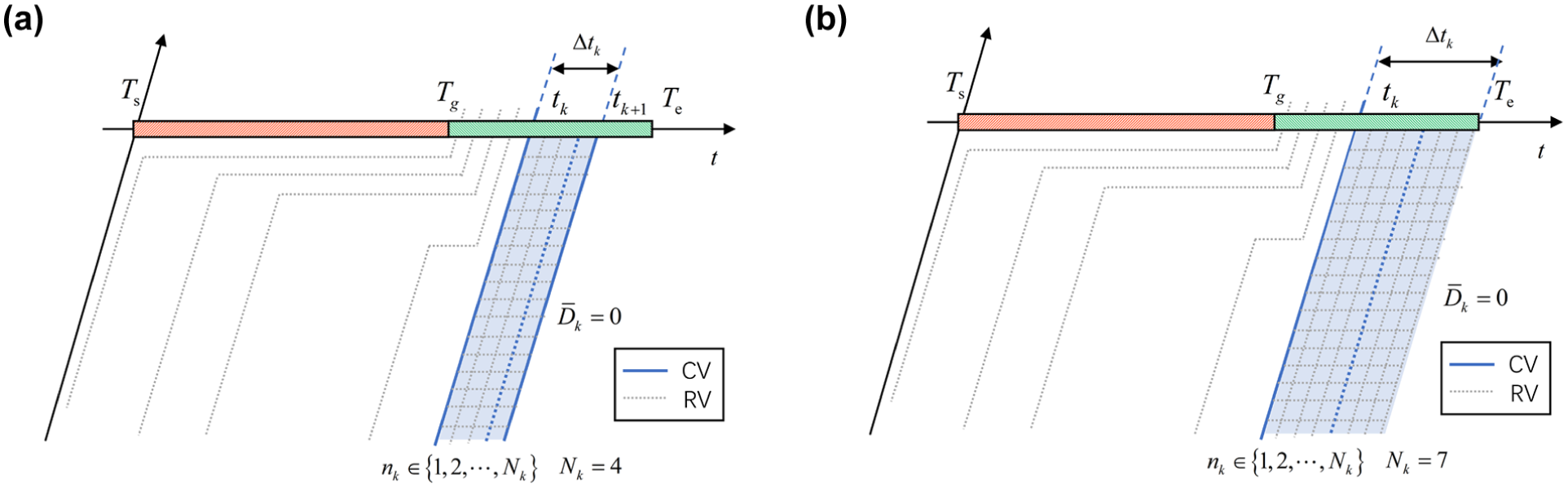
This study focuses on a signalized intersection with dynamic signal control in undersaturated traffic conditions. While the optimization strategy governing the signal changes is unknown, the resulting signal timing is observable. Vehicles traversing the intersection consist of two types: (1) observable CVs, whose trajectory data are available; and (2) unobservable regular vehicles (RVs), for which no direct trajectory information can be obtained. The sampling frequency is sufficient to ensure the timely and reliable extraction of CV states. The objective of this study is to estimate the average delay at the cycle level. The specific study scenario and representative trajectories are shown in Figure 1.
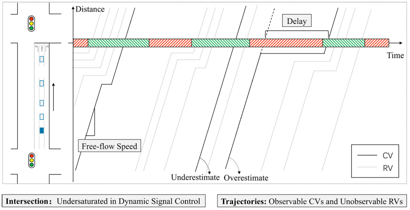
Research scenario.
To focus on the research difficulties and simplify the problem, the following assumptions are made in this study.
This study focuses on an isolated signalized intersection operating in undersaturated traffic conditions, where residual queues or queue spillback are not considered.
Traffic demand exhibits temporal variability and randomness; it is assumed to follow the same distribution across different days for a given TOD period.
All vehicles follow a homogeneous deterministic Newell’s car-following model (
22
). This assumption applies to urban traffic characterized by intermittent flow, where vehicle delays are caused by traffic signals inducing acceleration and deceleration and stopping, and vehicles have the main characteristic of frequent stopping.
Vehicle arrivals at different moments are assumed to be independent of each other. For each time interval
Estimation of Vehicle Arrival Distribution
Newellian Coordinate Transformation of Vehicle Trajectory Data
Building on the discrete formulation of Newell’s car-following theory, this study adopts the Newellian coordinate framework proposed by Wang et al. ( 8 ) to simplify vehicle movement modeling at intersections. Because urban traffic features interrupted flow, where stop-and-go is the dominant characteristic of vehicle trajectories, vehicle delay mainly comes from the stopping time caused by traffic signals and queuing. Under low CV penetration, uncertainty primarily stems from limited trajectory coverage and stochastic traffic demand. To address this, traffic dynamics are approximated using discrete arrival and departure events, ignoring individual vehicle behavioral variation.
Vehicle arrivals during each discrete time interval are modeled as Bernoulli processes, representing either zero or unit flow

where
The Newellian coordinates map real-world space–time points to a simplified time-flow grid, where horizontal resolution equals the time interval
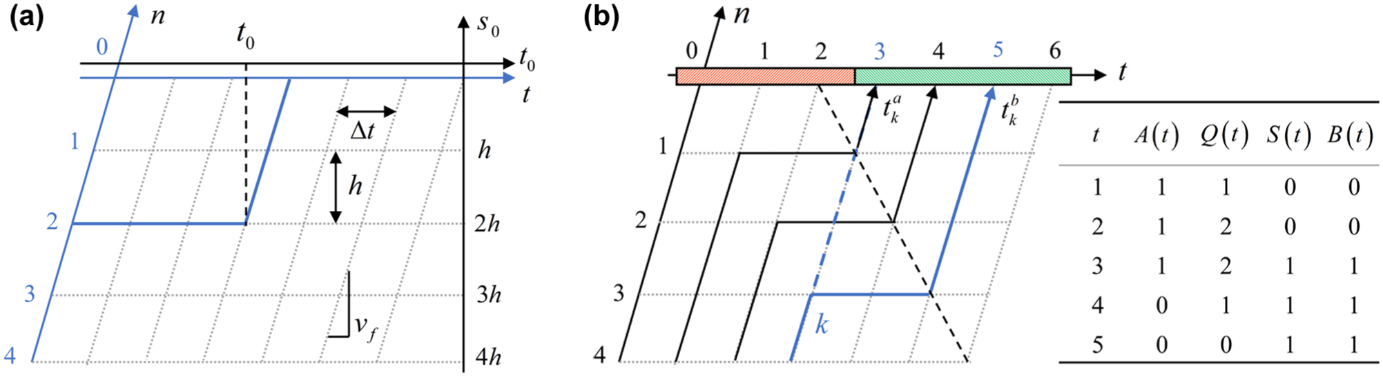
Vehicle trajectories in real-world time–space coordinates and Newellian coordinates: (a) Newellian coordinates; and (b) point-queue under Newellian coordinates.
The transformation from real-world coordinates

The key difference between real-world time–space coordinates and Newellian coordinates is that the latter use free-flow arrival time t instead of actual time. Vehicles in Newellian coordinates only travel along grid lines. Taking trajectory shown in Figure 2b
Estimation of Vehicle Arrival Distribution
To simplify the notation,
The trajectory data within a TOD period is shown in Figure 3. After transforming vehicle trajectories into Newellian coordinates, the arrival time t for each unit flow vehicle is easily obtained. Vehicle trajectories are aggregated in the TOD. Where
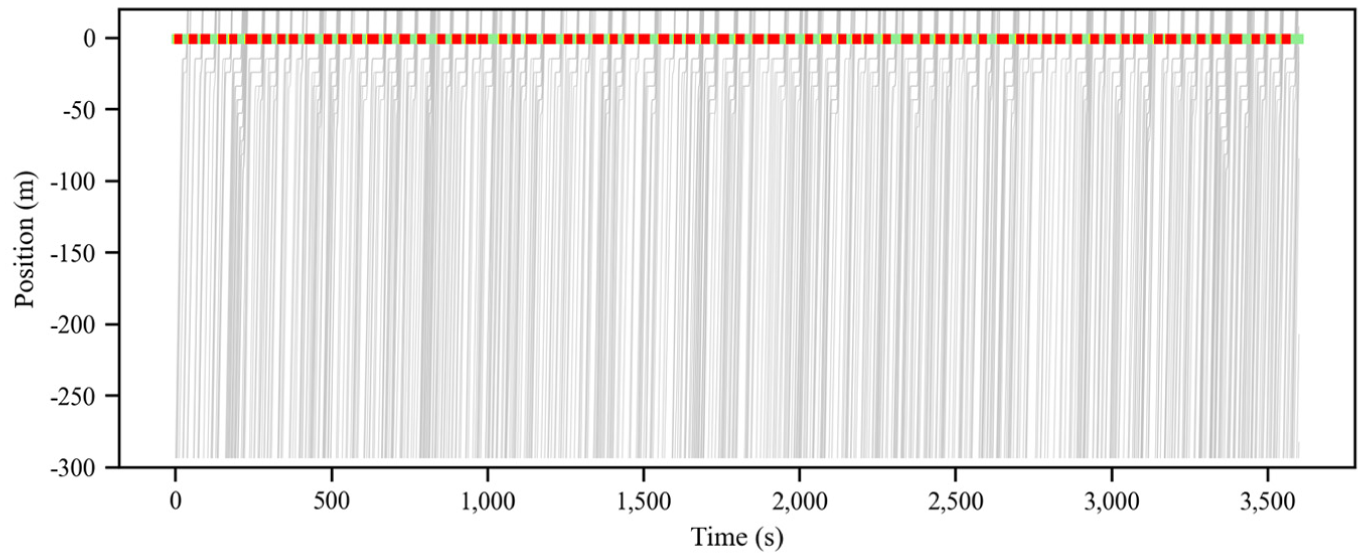
Vehicle trajectories within a TOD period.
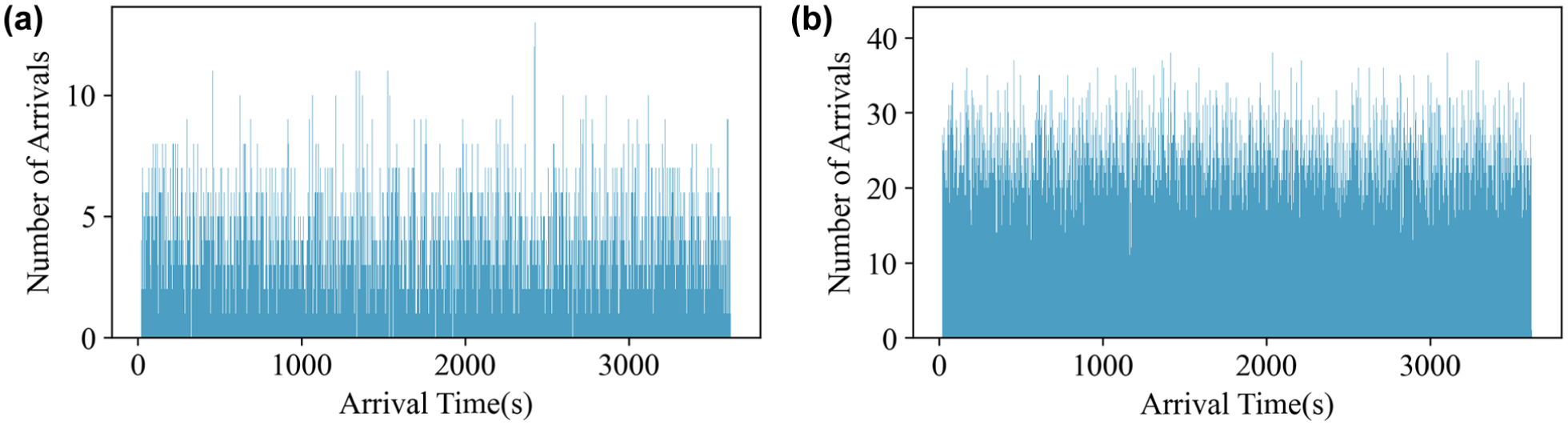
Histogram of
Many studies provide estimation methods of penetration rate (
24
,
25
). Therefore, the penetration rate of CVs at a specific intersection can be estimated using existing methods or field studies. Given the penetration rate
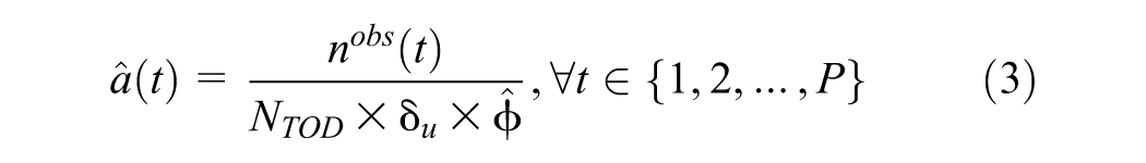
where
Cycle-by-Cycle Delay Estimation Model
Evolution of the Queued Vehicle Number
Let the research period be denoted as

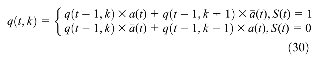
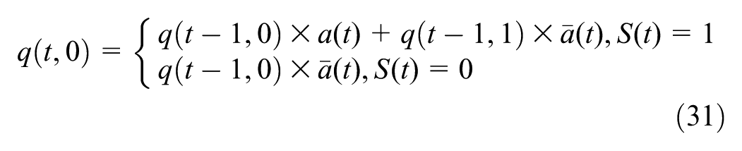
The Newellian coordinates can convert all vehicle trajectories into a point-queue. Let

The queued vehicles in Equation 5 are called point queues. The number of queued vehicles

Figure 2b shows a case study on the evolution of queued vehicle numbers over time using a stochastic point-queue. Vehicles arrive at times
Assuming the

where

Using the previous steps, the control delay of each queued vehicle can be derived via the stochastic point-queue model, providing a theoretical basis for the subsequent cycle-by-cycle average vehicle delay estimation method.
Cycle-by-Cycle Estimation of Average Vehicle Delay
Framework of Delay Estimation
In the Estimation of Vehicle Arrival Distribution section, vehicle arrivals within TOD are estimated using historical trajectory data, yielding the probability of vehicle arrivals at each moment in TOD. Delay estimation is then performed cycle-by-cycle within TOD based on these arrival probabilities and trajectories within the cycle. Trajectories in the cycle are those whose free-flow arrival time falls within the cycle (from the start of the red light to the end of the green light).
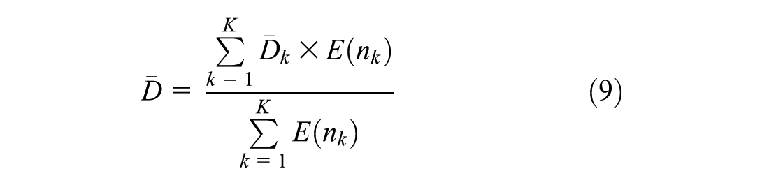
As shown in Figure 5, let
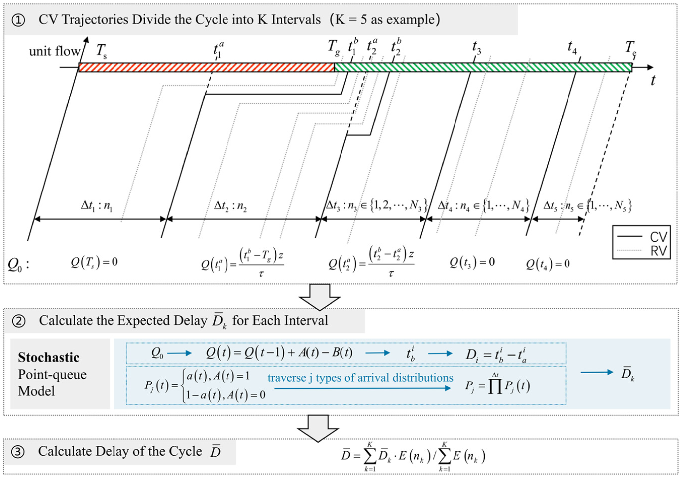
Cycle-by-cycle delay estimation framework.
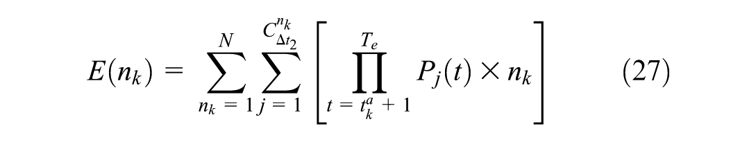
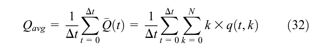
The method for estimating the average delay per cycle is as follows. Based on the observed arrival times of
Within each time interval, all possible arrival distributions are traversed. Calculate the initial number of queued vehicles
Scenario 1: Average Delay for Vehicles Before the First Queued CV
When the first observed trajectory in the cycle is a queued CV (Figure 6), let

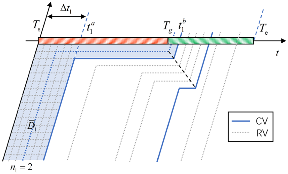
Before the first queued CV.
Let τ represent the saturated headway and

Within the time interval

Obtain the delays for
where

Scenario 2: Average Delay for Vehicles Before the First Non-Queued CV
When the first observed trajectory in the cycle is non-queued CV (Figure 7), the maximum number of vehicles passing before the first non-queued CV in the cycle is given by,

Before the first non-queued CV.
Therefore, the number of vehicles passing ahead of the CV during this interval is

Calculate the delays of
Scenario 3: Average Delay for Vehicles Between Two Queued CVs
When the interval is between two queued CVs (Figure 8), the number of vehicles arriving between two queued CVs (within the interval

Between two queued CVs.
For

The departure time of the
Calculate delays for these

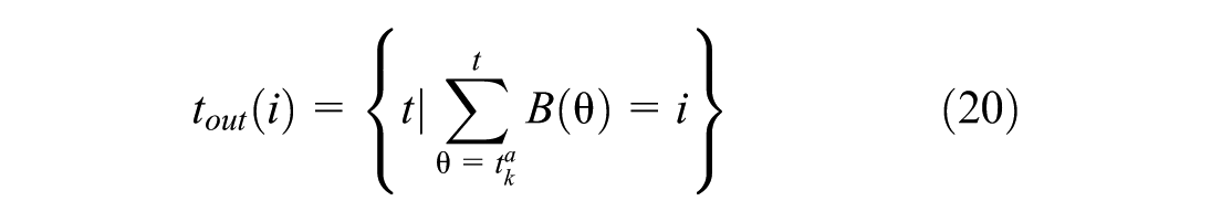
Scenario 4: Average Delay for Vehicles After Queued CV/Between Queued and Non-Queued CVs
When the interval is after a queued CV (Figure 9a) or between queued and non-queued CVs (Figure 9b), let

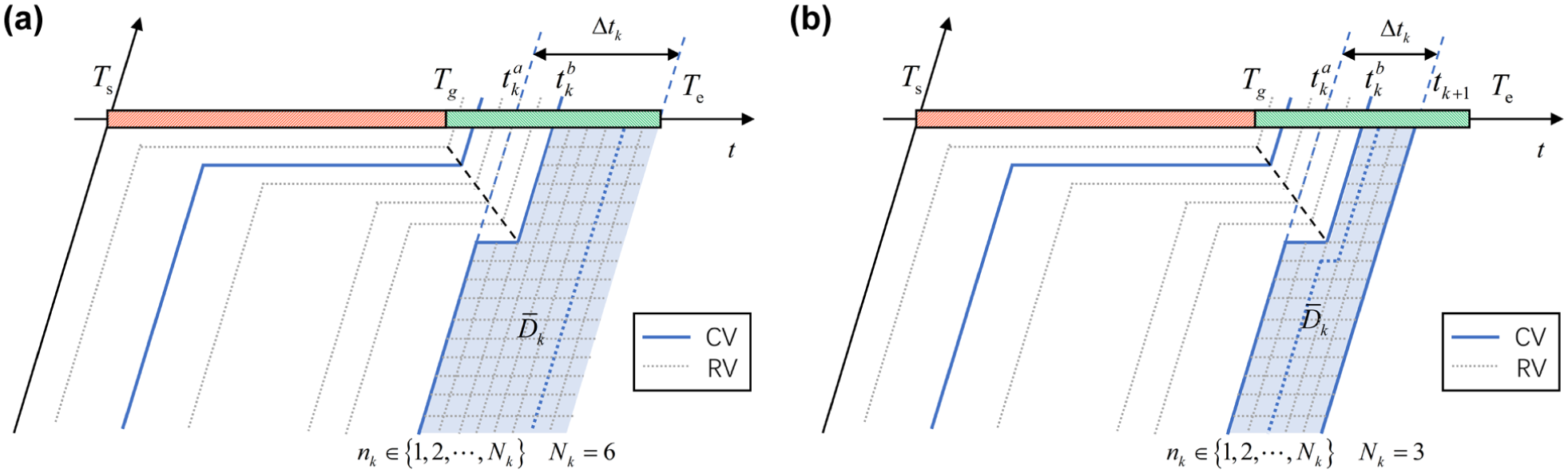
After the queued CV or between queued and non-queued CVs: (a) after the queued CV; and (b) between queued and non-queued CVs.
The maximum number of vehicles that can pass through in

Therefore, the number of vehicles passing through in interval

The departure time of the
Calculate delays for
where
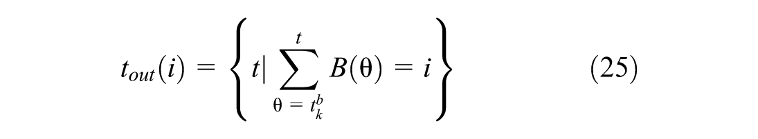
Scenario 5: Average Delay for Vehicles Between or After Non-Queued CVs
When the interval is between non-queued CVs (Figure 10a) or after a non-queued CV (Figure 10b), the maximum number of vehicles that can pass behind this CV in the cycle is given by,

Therefore, the number of vehicles passing behind the CV during this interval is

Between non-queued CVs or after non-queued CV: (a) between non-queued CVs; and (b) after non-queued CV.
Approximation of Evolution of the Queued Vehicle Number
Computational Burden Issues
Practical experiments identified an algorithmic bottleneck in the method in the Cycle-by-cycle Estimation of Average Vehicle Delay section. This method requires enumerating all possible vehicle arrival combinations, and as the cycle length increases, the number of combinations grows exponentially, particularly when estimating delays for
To resolve this, replacing the stochastic point-queue model with a deterministic one to calculate segmented delays across scenarios is proposed. This approach avoids enumerating all arrival combinations; instead, it directly incorporates vehicle arrival probabilities to compute the average number of queued vehicles. Using Little’s law, the average delay is derived by dividing the average number of queued vehicles by the average arrival rate. For short intervals, the original method remains highly accurate. For longer intervals, however, the exponential growth in combinations requires the optimization strategy, trading a small reduction in accuracy for an increase in algorithm speed.
In addition, if no CV trajectories are observed in a cycle, the only available posterior information is traffic light status. In these cases, delay estimation must rely on historical arrival distributions and signal status, requiring the proposed deterministic point-queue-based approximation to estimate delays.
Deterministic Point-Queue Model
The deterministic point-queue model here simplifies the stochastic point-queue model. The key difference is that the latter uses a discrete variable sequence
when
when
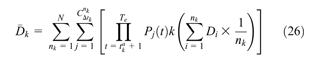
Approximation of Average Number of Queued Vehicles Within the Interval
Let the duration of the interval obtained by segmenting the cycle be
Approximation of Average Delay Within the Interval
The intersection is in an unsaturated state; therefore, because the number of vehicles arriving and leaving the system is approximately equal within a time period and is in a stable state, the average delay during the interval can be calculated according to Little’s law.

where

Numerical Experiments
Simulation Settings
To evaluate the performance of the proposed delay estimation method, this study uses the open-source traffic simulation software Simulation of Urban Mobility to create a dynamic signalized intersection environment. The simulation models a typical isolated two-way, eight-lane urban arterial intersection. The intersection employs vehicle-actuated signal control, which dynamically adjusts timing based on real time traffic demand, with a typical four-phase structure. Main parameters include a minimum green time of 5 s, a maximum green time of 50 s, a vehicle detection gap of 3.0 s, and a unit green extension of 3 s. Once a phase’s minimum green time elapses, green duration is extended by 3 s if vehicles are detected; the phase switches when no vehicles arrive or the maximum green time is reached. Therefore, each phase’s green time and the overall cycle length are dynamically determined by actual traffic demand, resulting in variable cycles.
Because the delay calculation for each movement at the intersection is independent, the delay estimation in the simulation experiments takes the through vehicles in the southbound lanes as an example. Given
Results and Discussion
Arrival Distribution Estimation
The accuracy of vehicle arrival probability estimates derived from historical data is estimated because this is critical prior information for delay estimation. Arrival probabilities (estimated by aggregating historical data) are compared with actual vehicle arrivals, analyzing how estimation performance varies with the number of trajectory aggregations
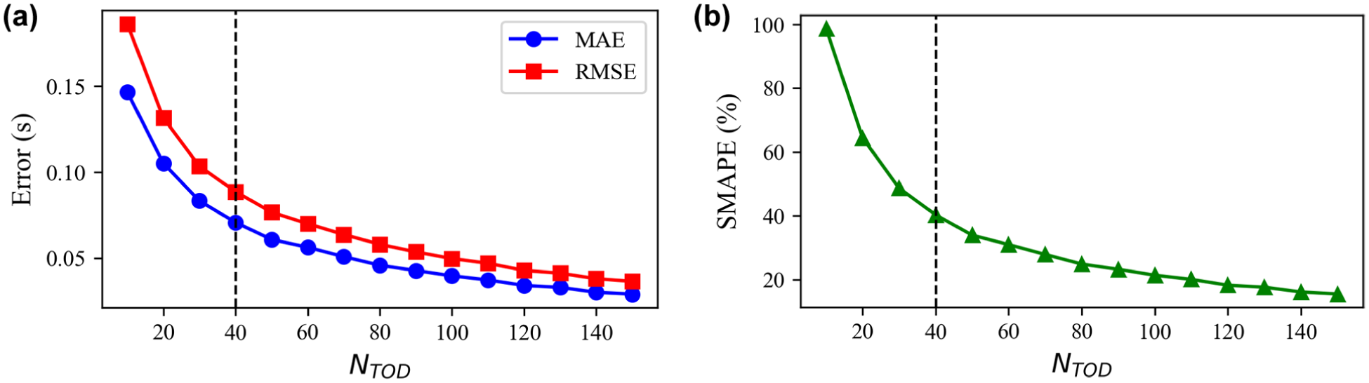
Arrival estimation errors under different numbers of trajectory aggregations
Cycle-by-Cycle Estimation of Average Vehicle Delay
To verify the performance of the proposed delay estimation model, it was compared with existing methods from the literature. Since there is little existing research on cycle-by-cycle delay estimation using vehicle trajectory data in dynamic signal control scenarios, the benchmark method selected is an existing historical trajectory-based delay method. This method is adapted from a fixed signal control delay estimation model in the literature ( 8 ), which estimates delay using the predicted arrival probability and the current cycle’s signal state. The key difference between the two methods is that the proposed cycle-by-cycle delay estimation method uses real time CVs trajectory data observed in the current cycle and classifies and analyzes this data based on its distribution. This enables more detailed and accurate delay estimation.
Cycle-by-Cycle Comparison of Model Performance
Figure 12 and Table 1 compare the delay estimation results of the proposed method based on historical aggregated and real time cycle trajectories with the existing methods based on historical aggregated trajectories in a simulation environment (3,600 s covering 70 cycles) under
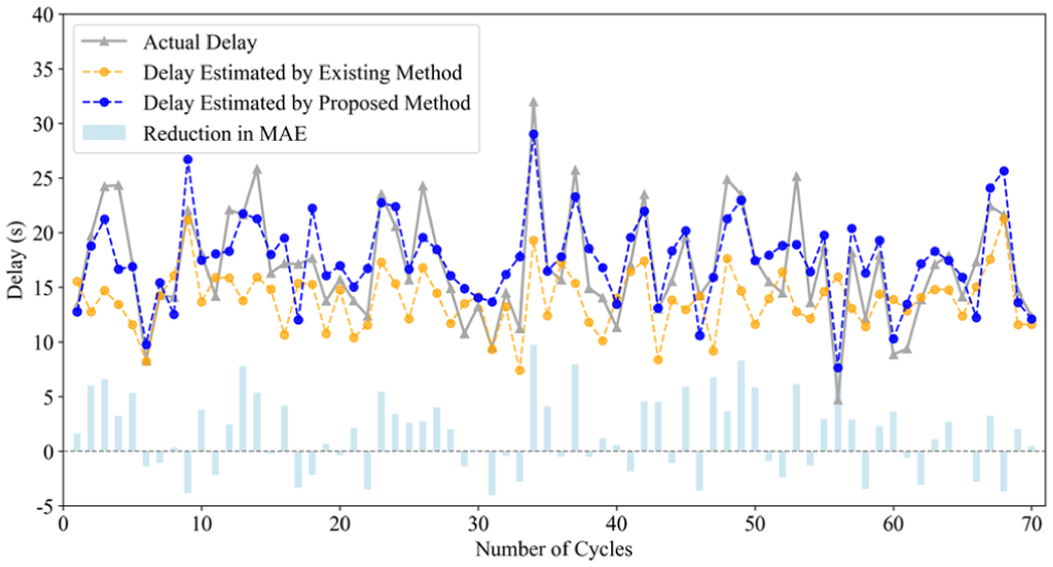
Comparison of the estimated delay between the proposed method and the benchmark method
Table 1 compares the average delay estimation error and error volatility of the proposed method and the benchmark method across 70 consecutive cycles. The proposed method has an MAE of 2.75 s and an RMSE of 3.41 s, representing reductions of 32.0% and 34.5% compared with the existing method. Its SMAPE also decreases from 25.29% to 17.40%, significantly lowering both absolute and relative delay estimation errors. In addition, the method’s low error variance indicates smaller error fluctuations over 70 cycles, effectively enhancing the robustness of cycle-by-cycle delay estimation across scenarios. Results show the proposed method reduces errors by over 30% and exhibits stronger stability, demonstrating significantly better performance than the benchmark method.
Cycle-by-Cycle Delay Estimation Results Comparison (
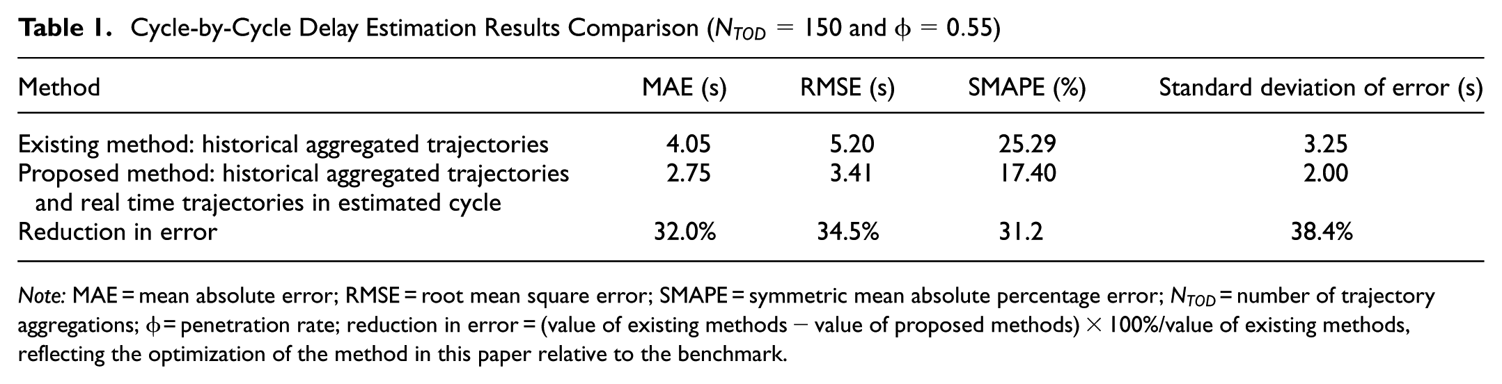
Note: MAE = mean absolute error; RMSE = root mean square error; SMAPE = symmetric mean absolute percentage error;
Comparison of Model Performance at Different Penetration Rates
Low, medium, and high CV penetration rates (5%–95%) are simulated using sampled trajectory data. Figure 13 compares the MAE of the proposed method and the benchmark method across these penetration rates. As can be seen from this figure: (1) as penetration rates decrease, the delay estimation errors of both methods do not rise significantly. This indicates the model is insensitive to reduced penetration and works well in low penetration scenarios; (2) higher penetration rates lead to slightly lower errors for both methods, though the trend is weak. This is probably because higher penetration improves vehicle arrival probability estimates (making traffic demand estimates more accurate) and increases the proportion of observed vehicles, enhancing delay estimation precision; and (3) the proposed method shows significantly smaller errors than the benchmark method, with higher estimation accuracy. This confirms that fusing historical data with real time trajectories effectively boosts estimation accuracy.
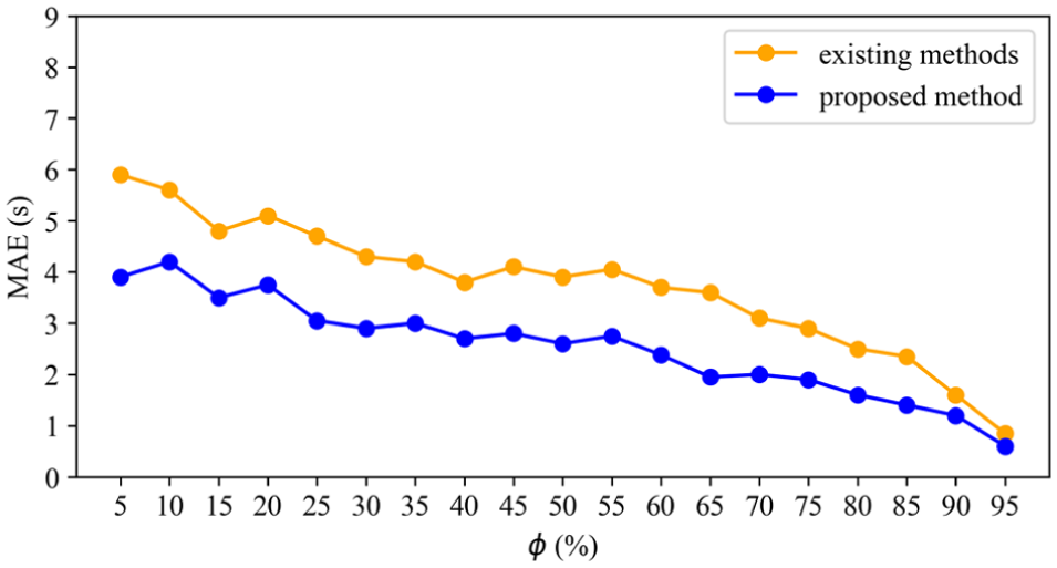
Comparison of delay estimation methods at different penetration rates (MAE).
Comparison of Model Performance Under Fluctuating Demands
Traffic demand was simulated from 7:00 to 10:00 a.m. during the morning peak to assess the robustness of delay estimation under fluctuating demand. Table 2 compares the estimation results of the existing method and the proposed method across different time periods. From 07:00 to 08:15 a.m., lower traffic flow led to higher delay estimation mean absolute percentage error (MAPE) for both methods because of small delay values. As traffic demand increased to the peak steady state (08:30–09:30 a.m.), the estimation errors decreased and became more stable. The proposed method achieved a lower average MAPE (14.6%) than the existing method (22.5%), and produced smaller errors in most time periods. These results indicate that the proposed model can better capture delay variations under time-varying traffic demand. In addition, historical data should be used with similar traffic demand distributions for parameter calibration to improve delay estimation accuracy in the new TOD.
Estimation Results of Time Period Delay
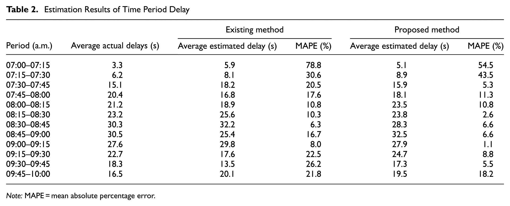
Note: MAPE = mean absolute percentage error.
Sensitivity Analysis
Estimation Error of Penetration Rate
This study estimates vehicle arrival probability using penetration rate calculated by existing methods or field surveys, so it is necessary to evaluate how the estimation accuracy of penetration rates affects delay estimation results. Figure 14 shows the effect of estimated penetration rate changes on delay estimation errors under
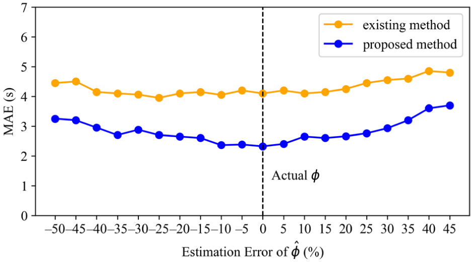
Effect of estimated penetration rate
Traffic Demand Distribution
Under V/C ratios of 0.3, 0.6, and 0.9 (corresponding to low, medium, and high demand levels in unsaturated conditions) for the southbound through lane of the intersection, the accuracy of delay estimation under two vehicle arrival patterns is analyzed: (1) uniform distribution; and (2) Poisson distributions. Figure 15 shows the estimated MAPE of delay across three traffic demand levels, which indicates the proposed method performs stably under different traffic demand levels and distributions. The penetration rate and arrival rate estimation at the high and medium demand levels are smaller overall than those at the low demand level. This is because more CV trajectories can be collected at higher demand levels. In addition, the delay value is lower at the low demand level.
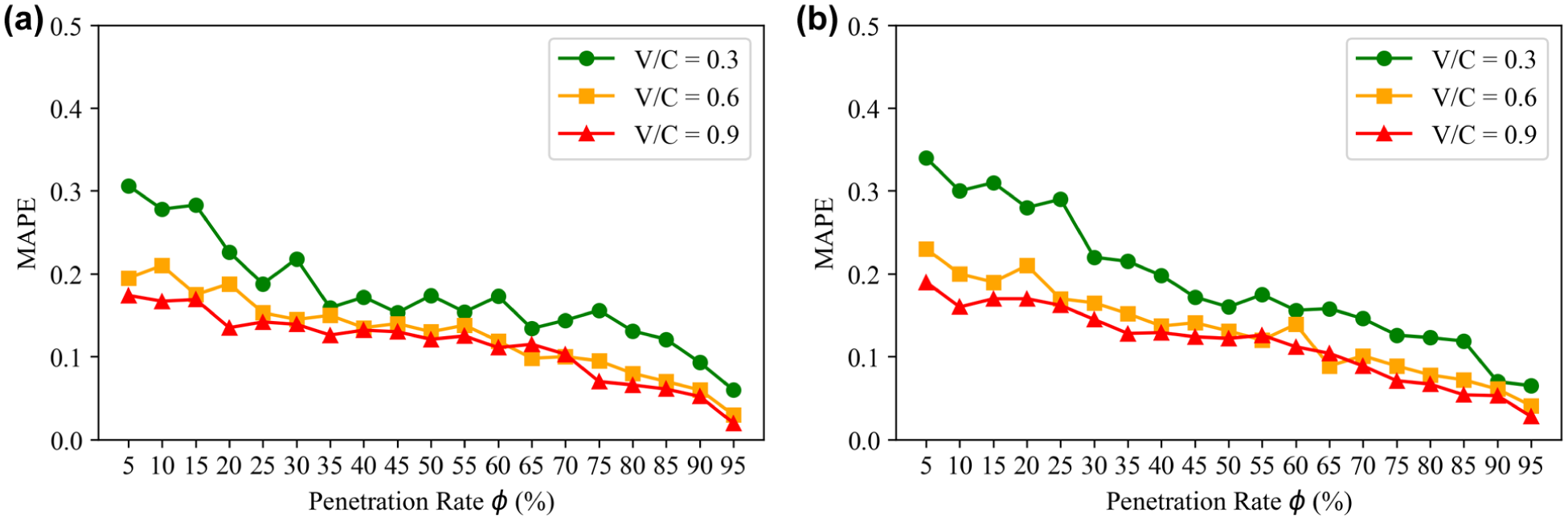
Variation in MAPE with penetration rate at different levels and distributions of demand: (a) uniform distribution; and (b) Possion distribution.
Conclusions
This study proposes a cycle-by-cycle delay estimation method for dynamic signalized intersections using CV trajectory data. The vehicle trajectory data is converted into Newellian coordinates. To cope with the low penetration rate, the vehicle arrival distribution is estimated by aggregating historical trajectories within a TOD period. Then, each cycle within the TOD under dynamic signal control is identified. Using the arrival time of each observed CV trajectory in the cycle, the cycle is divided into several time intervals (with all five possible scenarios discussed). From the trajectory data, the number of queued vehicles (or maximum value) in each interval is known. Then, based on a stochastic point-queue model, the evolution of the number of queued vehicles is used to analyze how vehicles gather and disperse at the intersection. A probabilistic delay estimation model is developed to estimate the average delay for each interval. Finally, the average delay of each interval is calculated to obtain the cycle-level delay. To address the algorithm’s time complexity, an approximated evolution of the number of queued vehicles based on a deterministic point-queue model is also proposed. This allows cycle-by-cycle estimation of average vehicle delay during the TOD period.
The simulation results show that: (1) the proposed method outperforms benchmark methods in delay estimation error and error stability (with errors reduced by over 30%), and achieves accurate estimation even with low CV penetration; (2) it is robust to estimation error of penetration rate. Because estimating vehicle arrival distribution during TOD depends on penetration rate, and field surveys or estimates may have errors, the method ensures stable delay results within a certain range of penetration rate errors; and (3) it performs stably under high, medium, and low traffic demand levels when the intersection is unsaturated.
This study verifies the applicability of the proposed model for isolated signalized intersections. However, real urban traffic systems often involve interactions among multiple intersections. Future research will extend the method to multi-intersection environments and investigate delay estimation under stochastic traffic conditions, where residual queues or occasional queue spillback may occur. In addition, subsequent research will account for heterogeneity in traffic flow caused by diverse vehicle types (e.g., heavy goods vehicles) to further enhance the model’s adaptability to real-world mixed traffic scenarios. In addition, the delay estimation results can be embedded in the adaptive signal control algorithm to improve traffic efficiency at dynamic signalized intersections.
Footnotes
Author Contributions
The authors confirm contribution to the paper as follows: study conception and design: X. Wu, C. Yu, W. Ma; data collection: X. Wu, C. Yu; analysis and interpretation of results: X. Wu, C. Yu, W. Ma, C. Li, Z. Su; draft manuscript preparation: X. Wu, C. Yu. All authors reviewed the results and approved the final version of the manuscript.
Declaration of Conflicting Interests
The authors declared no potential conflicts of interest with respect to the research, authorship, and/or publication of this article.
Funding
The authors disclosed receipt of the following financial support for the research, authorship, and/or publication of this article: This study was supported by the National Natural Science Foundation of China (Nos. 52325210, 52131204, and 52272336) and the Shanghai Academic Research Leader Program (No. 23XD1404200).