
Abstract
Accurate, network-wide traffic volume data is essential for effective transportation planning and policy development. While traditional count stations offer reliable measurements, the high cost of their installation and maintenance limits full network coverage. Existing estimation methods often rely on sparse or outdated data, constraining their scalability and accuracy. This study introduces a novel framework that integrates probe vehicle data, stationary counts, and machine learning to estimate traffic volumes via modeled penetration rates. Penetration rates are first computed at locations with observed data and filtered using the interquartile range method to remove outliers. These rates are then used to train an XGBoost model, with Shapley additive explanations employed to assess feature importance and enhance model interpretability. The framework was validated on 675 road segments in Edmonton, Alberta, with 95.11% of observations retained as valid data. A network-wide mean absolute percentage error of 18.19% was achieved, with higher accuracy observed on high-volume roads. These results demonstrate the framework’s scalability and utility for large-scale traffic volume estimation in data-scarce environments, offering transportation agencies a cost-effective alternative to sensor-based monitoring for infrastructure planning and investment prioritization.
Introduction
Traffic volume data are crucial for accurately evaluating transportation system performance, measuring congestion and delays, detecting real-time network disturbances, and analyzing traffic patterns during significant weather events ( 1 , 2 ). In particular, accurate annual average traffic volume statistics such as annual average daily traffic (AADT) and annual average weekday traffic (AAWDT) are critical, as they directly support infrastructure design, safety assessments, environmental analyses, and inform various policy decisions ( 3 ). In Canada, transportation agencies commonly employ permanent and short-term counting methods for traffic volume monitoring ( 4 ). Permanent counts are continuously operated throughout the year, aimed at capturing seasonal variations in traffic flow. Short-term counts, conducted across a larger number of sites, are used to collect representative traffic samples across a broader roadway network. However, full network coverage cannot be achieved by counting stations because of the high costs of installation and maintenance ( 5 ). Given the lack of comprehensive traffic volume observations across most urban road networks, traffic volume prediction is considered a more practical and feasible solution ( 6 , 7 ). As a result, estimating traffic volumes in uncovered or low-coverage areas to enable network-wide traffic assessment has become a key research focus in the transportation field.
One widely used approach for traffic volume estimation is the factor-based method, originally formalized by AASHTO in its Guidelines for Traffic Data Programs ( 8 ). While broadly applicable, the conventional AASHTO method exhibits limitations, including its assumption of equal weighting across days and requirement for complete daily data. To address these issues, Jessberger et al. ( 9 ) proposed an improved method that incorporates hourly aggregation, allowing for the inclusion of partial-day data. This approach, now commonly known as the FHWA method, has demonstrated enhanced accuracy and precision ( 9 , 10 ).
While the FHWA method is structurally simple and widely standardized, it is also constrained by several key limitations, including low feature dimensionality, strong dependence on data availability, and limited scalability. To address these challenges, researchers have applied multiple linear regression widely to enhance estimation accuracy through the incorporation of additional features and to extend coverage to areas with limited or no traffic count stations ( 11 – 14 ). The features used in previous studies can generally be categorized into three groups: spatial and locational characteristics, demographic and socioeconomic factors, and roadway attributes. Most of these features have been shown to be effective to varying degrees. However, given the complexity of real-world conditions, many features do not exhibit a linear relationship with traffic volume. As a result, more sophisticated analytical methods are needed, and numerous machine learning approaches have proven effective in capturing such nonlinear patterns ( 15 , 16 ).
These findings underscore the advantages of machine learning approaches over traditional methods for estimating traffic volume. Consequently, multiple studies have explored various machine learning techniques to further improve traffic volume estimation accuracy. Support vector regression (SVR) with data-dependent parameters was applied to estimate traffic volumes across the state of Tennessee. The model achieved an average MAPE of 2.26% in urban areas and 2.14% in rural areas, demonstrating high predictive accuracy ( 17 ). In another study, clustering was combined with SVR and random forest (RF) to further confirm the effectiveness of machine learning approaches in complex roadway environments ( 18 ). In addition, deep learning has been widely adopted in recent studies for traffic volume estimation. Long short-term memory (LSTM) networks have been frequently employed to capture temporal dependencies in traffic dynamics ( 19 ). Graph convolutional network (GCN) has been used to model spatial correlations within road networks ( 20 ). Given the highly dynamic and spatiotemporal nature of traffic systems, researchers have also incorporated attention mechanisms to enhance the ability of models to capture variable dependencies and proposed various attention-based extensions to improve model performance and interpretability ( 21 , 22 ).
Although many previously proposed traffic volume estimation methods have demonstrated satisfactory performance, they typically rely on long-term, stable historical data. In practical applications, counter deployment density and missing data often limit the ability of these methods to maintain accuracy. Moreover, most models are built on the assumption of periodic and stable traffic patterns, making them insensitive to abrupt behavioral changes ( 23 ). As a result, their predictive capabilities are significantly constrained when faced with sudden disruptions in travel behavior, such as those caused by the COVID-19 pandemic ( 24 ). In response to these challenges, attention has been increasingly directed toward the integration of emerging data sources to improve model adaptability to spatial heterogeneity and temporal variability.
Probe vehicle data, derived from GPS-enabled vehicles, provides the traffic counts necessary to understand and monitor traffic conditions across a road network and has demonstrated significant potential in enhancing traffic volume estimation. Sekuła et al. ( 25 ) integrated multidimensional probe vehicle data into traffic volume estimation and used an artificial neural network to model the relationship. Using probe data as core features, their approach outperformed the baseline profiling method with an average accuracy improvement of 24%. Zhang and Chen ( 26 ) processed probe vehicle data to derive the annual average daily truck probe AADTP and incorporated the data as an explanatory feature in a machine learning model. As a result, the median error and the mean absolute percent error (MAPE) decreased to 20% and 30% for the estimated truck AADT, respectively. Likewise, another study ( 27 ) incorporated probe vehicle data into the model as input features in two forms: annual average daily probe counts (AADP) and betweenness centrality derived from observed speeds. That study compared three machine learning methods, with RF ultimately selected as the preferred model. These results demonstrated that incorporating these two probe-based features significantly enhanced the accuracy of traffic volume estimation, with AADP identified as the most explanatory individual variable. In more recent work, Cottam et al. ( 28 ) showed that large-scale freeway traffic flow estimation was effectively supported by probe vehicle data. Specifically, they developed a dynamically weighted ensemble model using speed-related probe data as core input features, which achieved satisfactory estimation accuracy.
Beyond using probe data as model input features, several studies have explored scaling it directly to estimate traffic volumes. Chang and Cheon ( 29 ) assumed a strong correlation between probe data and actual traffic counts and proposed a locally weighted power-curve model to estimate AADT on uncovered segments. However, this approach is sensitive to data sparsity and may yield unreliable parameter estimates under limited observations. Another study estimated segment-level penetration rates by combining probe and counting station data, using machine learning to generalize rates across unmonitored locations ( 30 ). The study then applied these rates to scale probe counts in volume estimates. While this approach improved estimation precision relative to earlier methods, it is limited to hourly volumes. Hourly traffic volumes are generally easier to obtain, whereas reliable annual average traffic volume data are much more costly to collect. Under constrained resources, estimating annual average traffic volumes is therefore a more challenging task.
In summary, while volume estimations remain foundational, achieving accurate estimates at network scale remains a challenge. Factor-based methods depend on complete data and limited features, while machine learning offers flexibility but is vulnerable to data gaps and behavioral shifts. As such, probe vehicle data have emerged as a promising alternative because of their high spatial resolution and increasing availability. However, probe data represent only a subset of traffic and lack inherent volume information. Moreover, given that the collection method itself carries sampling errors, its reliability requires further clarification. Without reliable estimates of penetration rates, which represent the proportion of total traffic represented by probe vehicles, raw probe counts cannot be directly translated into accurate volume estimates. To address the aforementioned limitations, this study proposes a novel framework that estimates AAWDT by explicitly modeling segment-level penetration rates using matched count data and machine learning. By combining the scalability of probe sensing with the adaptability of modern estimation techniques, the proposed approach enables interpretable, network-wide traffic volume estimation under data-scarce conditions.
The remainder of this paper is organized as follows: the methodology section outlines the proposed framework for traffic volume estimation; the next section presents and discusses the results of the case study; and finally, the paper concludes with a summary of the key findings and contributions, along with suggestions for future research.
Methodology
This section outlines the proposed framework for annual average traffic volume estimation, details the methods employed in each step along with the underlying rationale, and presents the relevant implementation details. Figure 1 provides a comprehensive overview of the framework.
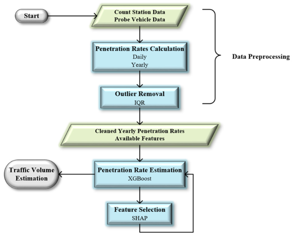
Workflow of the proposed traffic volume estimation framework.
As shown in Figure 1, this study uses two main data sources: count station data and probe vehicle data. The count station data consist of both long-term and short-term observations. Long-term count station data provide direct annual average traffic observations. In contrast, short-term count station data are first converted to annual average traffic volume using the FHWA method ( 31 ). To integrate the probe vehicle data, daily and annual penetration rates are estimated by spatially matching probe data locations with those of the count stations. To ensure data quality, outliers are subsequently removed using the interquartile range (IQR) method ( 32 ). An outlier is defined as a location where the daily and yearly penetration rates are significantly different, indicating a high level of uncertainty in the collected traffic counts. These data points are therefore excluded from the modeling process. The cleaned yearly penetration rates are the target variables for the following steps.
After removing outliers, all available features are input into the XGBoost (extreme gradient boosting) model for initial training, and SHAP (Shapley additive explanations) values are computed to interpret the importance of each feature ( 33 , 34 ). Counterintuitive and less important features are then excluded based on this analysis. Next, the cleaned data set along with the selected features are input into the XGBoost model again for retraining, to estimate penetration rates. These rates are then used in the penetration rate formula to derive the final traffic volume estimates. Detailed operational procedures for each step are elaborated on in the following sections.
Data Preprocessing
To support network-wide traffic volume estimation, the proposed approach first establishes a set of variables derived from both stationary counts and probe vehicle observations. These variables are used to compute annual traffic volumes, penetration rates, and outlier thresholds, which collectively form the basis for subsequent model training. Table 1 summarizes all relevant parameters, followed by a step-by-step description of the preprocessing procedure.
Parameter Descriptions
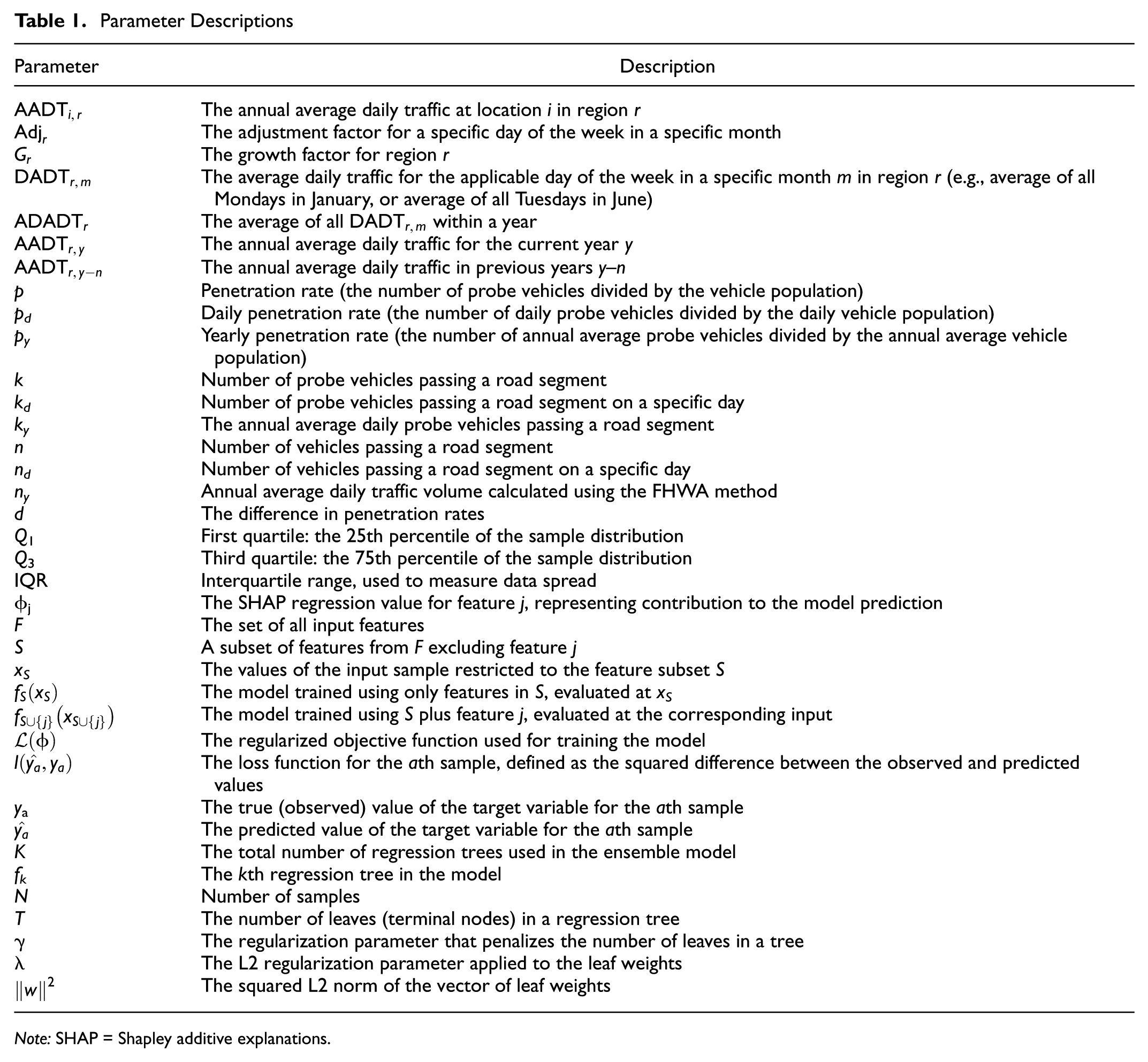
Note: SHAP = Shapley additive explanations.
To obtain annual-level traffic volumes, short-term counts of average daily traffic (ADT) are converted to annual average traffic volume by applying both adjustment and growth factors computed from a long-term/permanent count station within the corresponding region. This conversion method is a variation of the Traffic Monitoring Guide (FHWA 2022) standard formula ( 31 ). AADT volume is calculated using Equation 1.

An adjustment factor corrects for temporal variation by normalizing day-specific counts against annual patterns, particularly in cases where certain days experience unusually high or low traffic volume. A growth factor is applied if the short-term count was collected in a previous year, to account for observed trends in traffic growth or decline over time. Although using the FHWA method to calculate the annual average traffic volume may introduce some errors, such errors are considered unavoidable in this study and are excluded from the error analysis. The adjustment and growth factors are calculated using Equation 2.

Since probe vehicle data are available year-round, both annual average traffic volume and daily traffic volume can be directly derived. In contrast, as previously described, annual average traffic volume from short-term count station data is estimated using its daily traffic observation and the FHWA method. Based on this, both daily and annual penetration rates for each road segment can be calculated using Equation 3.

According to Equation 3, because the true traffic volume is nonzero, the penetration rate can be zero only when the probe count is zero. A zero probe count may arise from multiple causes, primarily sampling variability or device-related anomalies. As such, all observations exhibiting a penetration rate of zero were removed during preprocessing to ensure data representativeness. Since the annual average traffic volume is estimated from the daily traffic volume recorded by short-term count stations, potential errors (beyond those introduced by the FHWA method) may also arise from inaccuracies in the daily traffic measurements themselves. This error may be influenced by road conditions on the day measurements are taken, seasonal factors, or specific segment characteristics (e.g., proximity to parks). Furthermore, errors may also exist in the probe vehicle data. As not all vehicles are equipped with GPS devices, the number of detectable vehicles may be subject to sampling bias. In addition, environmental conditions can affect GPS signals, leading to potential trajectory deviations. To ensure maximum data reliability, the difference in penetration rates is used to filter out potentially erroneous data, in accordance with Equation 4.

If all errors remain within an acceptable range, the resulting penetration rate difference will also fall within a reasonable interval. However, the presence of any single excessive error is likely to cause this difference to deviate toward an extreme value. Based on this behavior, outliers in the penetration rate difference are identified and removed, and the remaining road segments are treated as reliable ground truth in this study.
The IQR method has been widely used for outlier detection in various data sets ( 32 ). It is particularly robust when applied to skewed data distributions. In this study, the variable of interest is the penetration rate difference, which exhibits inherent variability. This makes the IQR method a suitable choice. Therefore, the proposed framework uses the IQR method for outlier detection, as shown in Equations 5 to 7.


Any penetration rate difference greater than the upper bound or less than the lower bound is considered an outlier. The corresponding data points are removed from the data set. The data preprocessing stage is thus concluded following the removal of outliers.
Penetration Rate Estimation
Although various predictive models can be employed to capture the nonlinear relationship between traffic volume and its covariates, this study adopts XGBoost, a state-of-the-art, tree-based, ensemble learning algorithm. XGBoost integrates regularized objectives with system-level optimization, enabling fast, scalable learning while effectively mitigating overfitting ( 33 ). Its proven performance on large-scale, high-dimensional structured data makes it especially suitable for traffic volume estimation tasks.
Given the large number of features and complex interactions involved, XGBoost is used here both for penetration rate prediction and implicit feature selection, offering a robust, generalizable approach without requiring extensive manual tuning.
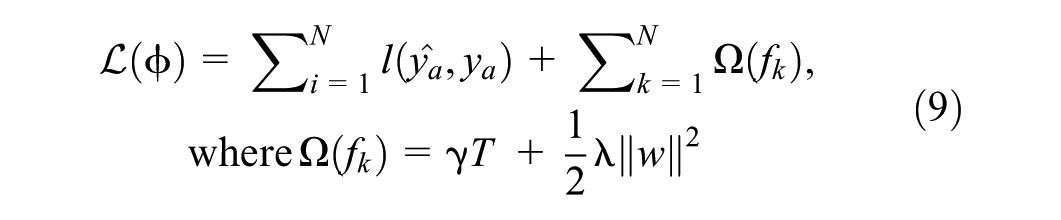
To operationalize this approach, the model is constructed using the Python XGBoost library ( 34 ). The model is trained by minimizing a regularized objective function, with the default squared error (Equation 8) adopted as the loss function in this study. The objective function used in this study is shown in Equation 9.

In practical implementation, key hyperparameters, such as the maximum tree depth and the number of iterations, are initially defined manually. To enhance model performance, a relatively wide hyperparameter search space is subsequently specified. GridSearchCV from Scikit-learn ( 35 ) is then employed to systematically perform cross validation over this predefined parameter grid, evaluating all parameter combinations exhaustively. Ultimately, the combination demonstrating optimal performance is selected for use in the model.
After the penetration rate is estimated, the final traffic volume is derived in accordance with Equation 10, allowing the results to be translated back to the volume level.

Feature Selection
The XGBoost model accommodates a wide range of potential input features, including geographic attributes, road characteristics, and contextual variables such as population density and employment levels (11–14). While prior studies highlight the relevance of these features, their generalizability across regions may be limited. As such, feature selection should be context-specific rather than based solely on existing literature.
Effective feature selection in this study is guided by two criteria: predictive contribution and interpretability. SHAP, a model-agnostic method based on cooperative game theory, is used to meet both criteria. SHAP quantifies the average marginal effect of each feature across all possible feature combinations ( 36 ). The SHAP values are formally defined using Equation 11.
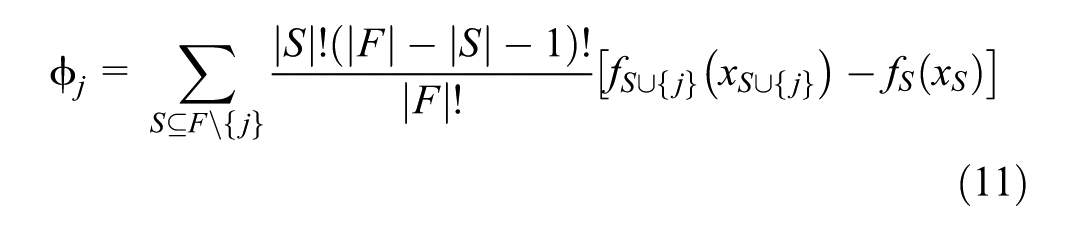
In practical implementations, the SHAP Python library is commonly employed ( 37 ). The magnitude of each SHAP value indicates feature importance, while the sign reflects its directional impact on predictions. This dual insight allows identification of features with limited contribution or those exhibiting counterintuitive effects.
All candidate features are initially included in the XGBoost model. SHAP values are then analyzed to compute the mean absolute contribution of each feature. Less important variables are removed, and those with signs misaligned with domain expectations are also excluded. The refined feature set is then used for final model training.
Case Study
To validate the proposed framework, a real-world case study was conducted in Edmonton, Alberta, Canada. This study focuses on estimating AAWDT, defined as “the average 24-h volume occurring on weekdays over a full year” ( 38 ), which is essential for supporting transportation planning and infrastructure development across the city. This section outlines the study area, data sources, and input features used in the analysis.
Study Area and Data Description
In this study, a diverse range of data sources was compiled and processed. The data sources include: internally collected data from the City of Edmonton (CoE) Mobility Monitoring and Analysis Department; the CoE’s Open Data Portal ( 39 ); and data from Statistics Canada ( 40 ). Figure 2 illustrates the spatial distribution of the available data across the city. The data set used in this study consists of 675 known data points across the entire CoE, covering the period from 2022 to 2024.
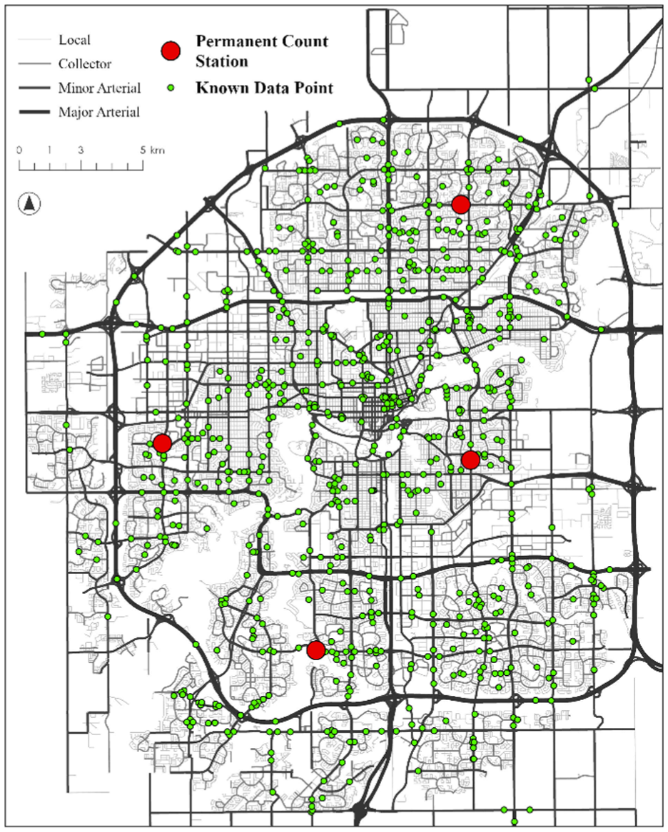
Spatial distribution of known data points within the study area.
In Figure 2, the red dots indicate known data points. In this study, “probe data” refers specifically to traffic volumes from probe vehicles. The probe data for all 675 known points used in this study were obtained from TomTom ( 41 ), for which traffic volumes are derived using aggregated GPS traces. These data supported the computation of daily and annual penetration rates, which in turn were used to derive AAWDT estimates. Descriptive statistics of the traffic volume data across both ground truth (CoE short-term counts) and probe data are summarized in Table 2.
Summary Statistics of Traffic Volume Data
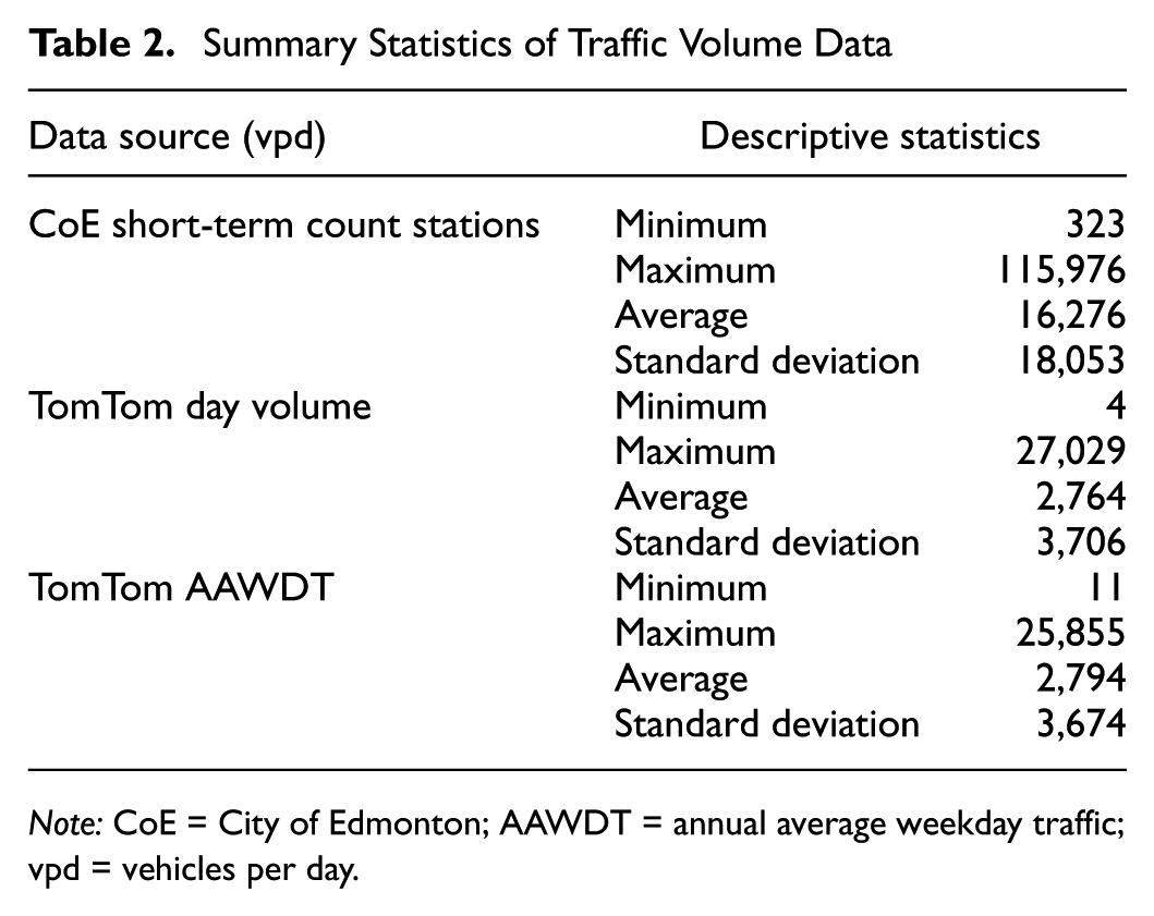
Note: CoE = City of Edmonton; AAWDT = annual average weekday traffic; vpd = vehicles per day.
To develop the predictive model, a set of spatial, operational, and contextual input features was assembled for each observation point. These features include speed limit, latitude, longitude, road class, region, number of lanes, employment rate, and population density (per square kilometer). A unique feature introduced in this study is “road segment type,” which distinguishes between two forms of ground truth data. Segments directly monitored by short-term count stations are labeled as “midblock,” while segments estimated using intersection balancing (based on upstream and downstream flows) are classified as “estimation.”
Among the remaining features, employment rate and population density were obtained from Statistics Canada ( 42 , 43 ), the speed limit was obtained from the CoE’s Open Data Portal ( 44 ), and the rest were internal data sourced from the CoE Mobility Monitoring and Analysis Department.
Results and Discussion
In this section, the results derived from sequentially applying the data through the proposed methodology are analyzed and discussed. Based on the method proposed in this study, AAWDT, daily penetration rate, and yearly penetration rate were calculated in succession. Data cleaning was carried out using the IQR method as described in the methodology section. Figure 3 illustrates the distribution of penetration rate differences and the outliers removed using the IQR method.
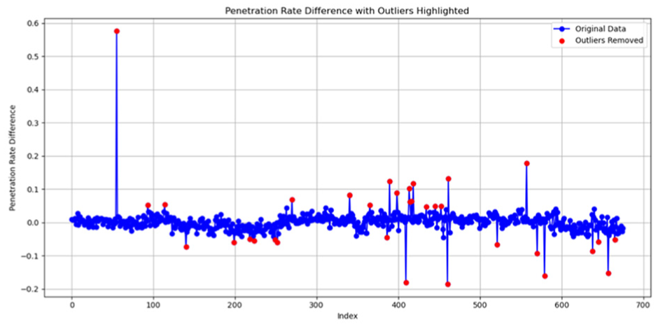
IQR-based outlier removal applied to penetration rate differences.
As shown in Figure 3, most of the penetration rate differences are concentrated within the range of −0.1 to 0.1. The data show only a small number of clearly identifiable outliers, which was consistent with expectations. The IQR method was then applied to detect and remove these outliers. As a result, a total of 33 data points were removed. The subsequent analysis in this study was conducted using the remaining 642 data records. The penetration rate distribution of the remaining 642 observations is shown in Figure 4. It can be observed that higher penetration rates are more likely to be associated with higher class roads. Because higher class roads are typically characterized by denser count station coverage and higher traffic volumes, it may be concluded that higher accuracy in penetration rate prediction was generally achieved on these segments and improved traffic volume estimation accuracy is consequently supported.
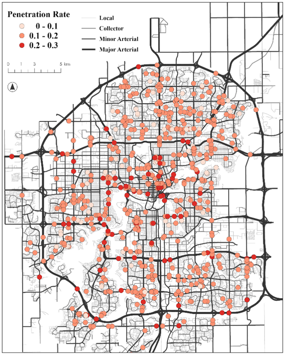
Penetration rate distribution.
For high-volume roads, a given penetration rate error was translated into a larger absolute traffic volume error than on low-volume roads. Conversely, on lower class roads, larger penetration rate errors were often observed, but a smaller adverse effect on overall traffic volume estimation was produced because the corresponding traffic volume scale was lower. Therefore, a practical advantage of penetration-rate-based estimation was reflected in the relatively higher penetration rate accuracy being achieved on segments which had a greater impact on estimation errors, while larger penetration rate errors on low-volume roads contributed less to total estimation errors.
During the modeling process, categorical features were processed using one-hot encoding, and all features were subsequently input into the XGBoost model for training and SHAP-based interpretation. The hyperparameter search space was defined as follows: the number of boosting trees was set to 20, 50, and 100; the maximum tree depth was set to 3 and 5; and the learning rate was set to 0.05 and 0.1. Feature importance rankings were derived from the mean absolute SHAP values. Figure 5 illustrates the feature importance ranking for all input features.
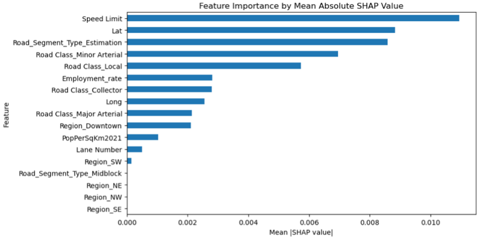
SHAP-based ranking of feature importance for the XGBoost model.
As shown in Figure 5, region-based features contributed minimally to model output, suggesting limited predictive value or redundancy with other spatial variables such as latitude, longitude, and road class. Although the Downtown indicator showed marginal influence, its effect was likely subsumed by these other spatial features. To reduce feature redundancy and simplify the model, all region indicators were removed. Although the SHAP value of “Road_Segment_Type_Midblock” also appeared negligible, this feature was specifically used in this study to distinguish between directly measured midblock volumes and volumes estimated from intersections, because it can enhance the model’s generalizability and interpretability.
After these adjustments, the model was retrained, and SHAP values were recalculated. In this second round, a SHAP summary plot was used (Figure 6) that accounts for both magnitude and direction of influence for each feature.
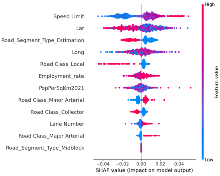
SHAP summary plot of all updated features.
As shown in Figure 6, the refined feature set produced results that align with domain expectations. For example, higher speed limits were generally associated with higher penetration rates, which is consistent with our observation that high penetration rates were more common on higher class roads, where speed limits are typically higher. Notably, speed limit, road class, and geographic coordinates (latitude and longitude) emerged as the strongest predictors of penetration rate. Among these features, direct associations with penetration rate were observed for speed limit and road class, whereas strong effects of geographic coordinates were likely attributable to spatial autocorrelation in traffic volume. Because this study targeted network-wide traffic volume completion under sparse data conditions, this spatial dependence was leveraged to improve estimation at nearby locations, thereby enhancing overall predictive accuracy. These findings confirm that the model effectively captures interpretable and operationally meaningful relationships.
On completion of the feature selection process, the filtered data set and retained features were input into the XGBoost model for training and prediction. To reduce random variability while evaluating the predictive performance, a standard random 10-fold cross validation ( 45 ) was employed. Each fold uses nine subsets of data for training and one subset for validation, rotating through all 10 subsets. The random 10-fold cross validation was selected because the primary objective of the study was network interpolation; in particular, this study focused on the estimation of traffic volumes for uncovered road segments located between existing distributed monitoring points within the same city. Under this objective, random 10-fold cross validation was considered the most appropriate validation approach, as it most closely simulates the practical scenario of randomly missing data within a monitored network and therefore provides an estimate that is most representative of the expected operational performance.
To provide a clearer and more intuitive evaluation of model performance, mean absolute error (MAE) (defined in Equation 12) and MAPE (Equation 13) are used. MAE offers a direct measure of error magnitude and helps reveal the distribution and potential sources of error. MAPE highlights the relative magnitude of error and is particularly useful for assessing predictions across a wide range of values. MAE and MAPE have been widely applied in the evaluation of traffic volume estimation results, and both are well suited for evaluating model performance in the context of traffic volume estimation. Therefore, these two metrics were used in this study.


Figure 7 presents the spatial distributions of MAPE, in which the volumes are classified using the natural breaks method ( 46 ). The results show that the predicted and observed AAWDT exhibit similar value ranges and spatial patterns, generally reflecting the accuracy of the prediction.
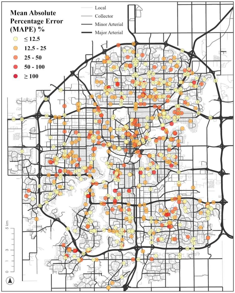
Spatial distributions of MAPE.
Based on 10-fold cross validation, the MAPE consistently fell within a range of 15% to 22%, indicating model stability. To facilitate overall evaluation, the subsequent results were obtained by averaging the outcomes of the 10-fold cross validation. Given the substantial variation in AAWDT across different road segments and drawing on insights from previous literature ( 30 ), performance metrics were evaluated both for the overall data set and stratified by road class. Specifically, MAE and MAPE were computed within each road class to provide a more nuanced assessment of model performance. The detailed results are presented in Table 3.
Model Evaluation Results
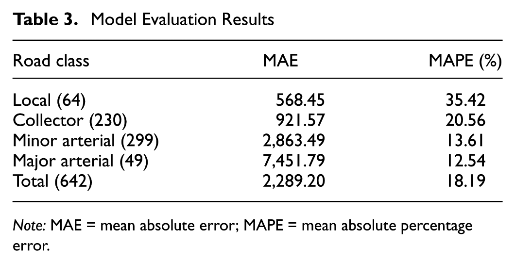
Note: MAE = mean absolute error; MAPE = mean absolute percentage error.
To illustrate the distribution and sources of prediction errors, the MAE values for all data points were grouped by road class and presented using box plots (Figure 8). Summary statistics including the mean, minimum, maximum, and standard deviation of MAE were also reported for each road class.
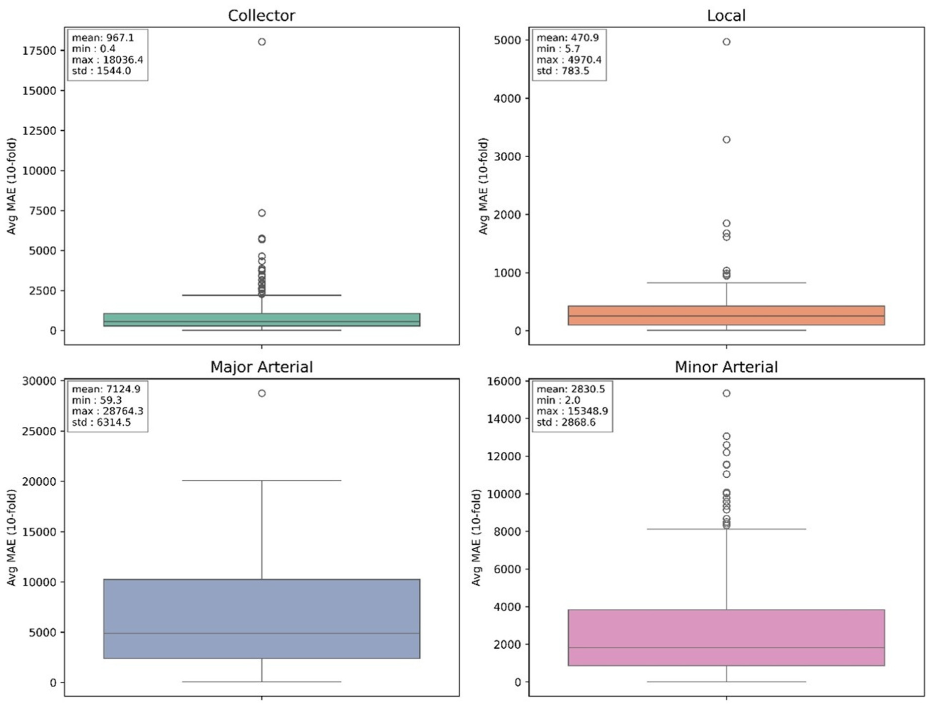
Boxplot of MAE grouped by road class.
As shown in Figure 8, although Major Arterial exhibits the highest mean MAE values, its error distribution is the most stable among all road classes. Moreover, as indicated in Table 3, this class also has the lowest MAPE, suggesting relatively high reliability in both absolute and relative terms. In contrast, the other three road classes demonstrate varying degrees of extreme error values. For instance, while Minor Arterial presents a MAPE comparable to Major Arterial, it exhibits greater variability, indicating less consistent model performance. A similar pattern is observed for Collector roads, likely because of the inability of road class alone to fully capture the heterogeneity in traffic patterns. Given that the Minor Arterial and Collector classes contain a relatively large number of data points, greater error dispersion is to be expected. On the other hand, the Local class contains fewer samples, which may hinder the model’s ability to learn generalizable patterns for the class.
In addition to the lower traffic volumes and limited availability of probe data, traffic counters are mainly installed on critical road segments, leading to fewer devices and imbalanced spatial distribution on lower-volume roads. Consequently, the insufficient training data from these areas results in an inability to capture accurate relationships, thereby reducing the prediction accuracy. Further, because the calculation of the MAPE is based on observed values, roads with lower traffic volumes and smaller observed counts (e.g., local roads) tend to produce higher MAPE values even when the absolute or relative errors are small. In other words, MAPE can exaggerate apparent model errors for low-volume segments and is not always a robust indicator of predictive accuracy in such cases. The acceptable MAPE ranges reported in the literature, which vary by traffic volume, further support this observation. Therefore, future studies should incorporate additional evaluation metrics to provide a more comprehensive and accurate assessment of model performance.
Given differences in study scope and data accessibility, direct comparison between the results obtained in this study and those reported in previous literature was considered difficult. In earlier studies, strong performance was often achieved when probe vehicle data were directly included as features and traffic volume was predicted using machine learning models. To demonstrate the practical improvement provided by the proposed framework, an additional experiment was conducted using the same data set without introducing the penetration rate. For this round, probe vehicle data were added directly to the feature set, traffic volume was predicted with XGBoost, and all remaining settings were kept identical. Under this set-up, an overall MAPE of 28.79% was obtained. By comparison, an overall MAPE of 18.19% was achieved with the proposed framework, indicating a substantial improvement in prediction accuracy. A likely explanation is that, without penetration-rate-based data cleaning, unreliable probe observations cannot be filtered out effectively. Because probe vehicle data are inherently affected by sampling variability introduced during data collection, data cleaning is widely recognized as a major practical challenge. In this study, penetration rate was introduced to connect probe vehicle observations with true traffic volume, and data cleaning was performed by leveraging traffic-volume-related characteristics.
To validate the effectiveness of the cleaning step, a follow-up experiment was performed on the cleaned data set, in which probe vehicle data were again directly included in the feature set. The overall MAPE was reduced to 19.62%, further confirming the effectiveness of the data cleaning process. The results obtained through penetration rate prediction were still slightly better than those obtained through direct traffic volume prediction. This difference may be attributed to the higher penetration rate accuracy being achieved on higher class roads, which contributed more to the overall error. Overall, it was demonstrated that the proposed framework can improve prediction accuracy while simultaneously enabling effective data cleaning.
To further contextualize these results, prior studies suggest that acceptable MAPE thresholds vary by traffic volume: 30% to 50% for low-volume roads, 20% to 25% for mid-volume, and 10% to 15% for high-volume segments ( 47 ). Since actual volume-based classification was unavailable, road class was used as a proxy, following definitions from the New York State Department of Transportation ( 48 ), with Local roads mapped to low-volume, Collectors to mid-volume, and Arterials to high-volume. Based on this mapping, all classes in the current study fall within their respective acceptable MAPE ranges. Notably, the framework not only satisfied these benchmarks, but it also frequently surpassed them, particularly on arterial roads, where MAPE values approach the lower bound of accepted thresholds. This level of performance affirms the proposed model’s robustness and operational viability, even under data-scarce conditions. Overall, the findings reinforce the practical applicability of the proposed framework for network-wide traffic volume estimation across varied roadway contexts.
Conclusions
This study developed a systematic framework for estimating network-wide traffic volumes by integrating limited stationary counts with probe vehicle data. Initially, the FHWA method was used to convert short-term counts into annual average traffic volumes, serving as ground truth for model calibration. To ensure data quality, penetration rate discrepancies between daily and annual levels were assessed, and statistical outliers were removed using the IQR method. SHAP-based interpretation was then applied to an XGBoost model to identify and exclude irrelevant or inconsistent features, thereby improving model interpretability and robustness. Penetration rates were then predicted using the refined XGBoost model, and final volume estimates were computed by scaling observed probe counts with the predicted penetration rates.
To evaluate the feasibility and practicality of the proposed framework, a case study was conducted using traffic and census data from the City of Edmonton covering the period of 2022 to 2024. The results demonstrate that the overall MAPE of the estimated traffic volumes reached 18%. Specifically, the MAPE for major and minor arterials was approximately 13%, while collector roads exhibited a MAPE of around 20%. For local roads, the MAPE increased to approximately 35%, indicating that estimation errors tend to increase as traffic volumes decrease. Overall, since all MAPE values remained within acceptable ranges as identified in previous studies, the findings confirm the effectiveness of the proposed framework. A further comparison was conducted between the proposed framework and the approach in which probe vehicle data were directly used as input features. The results further demonstrated both the effectiveness of the data cleaning process and the superior performance of the proposed method.
Based on the Edmonton case study, it can be inferred that in any region where data are limited but probe vehicle data are accessible, such data can serve as a valuable supplementary source to enhance the accuracy of network-wide traffic volume estimation. It also indicates that the proposed approach provides a practical and transferable methodology for applications in data-limited environments. However, since a factor-based procedure was first applied to obtain annual average traffic volumes, transferring to another region requires the availability of long-term observations from which the required factors can be derived. Furthermore, because penetration rates are highly sensitive to geographic characteristics, a sufficient amount of local probe vehicle data and short-term count observations must be obtained for the relationships between penetration rates and the associated features to be accurately captured by the model. Therefore, the framework is recommended primarily for application in a large-scale implementation where such data are more readily available.
Several directions for future research are worth exploring. First, the potential propagation of error from the FHWA method was not quantified in this study. Future work could investigate alternative methods for annual volume derivation to reduce dependency on potentially biased adjustment factors. Another promising direction involves conducting a deeper investigation of the outliers identified by the data cleaning method proposed in this study, while incorporating more advanced cleaning techniques to further improve data reliability. While this study used only probe vehicle traffic volumes as input data, future research may consider integrating additional types of probe data, such as speed, heading, or origin–destination information, to enrich the feature space and enhance estimation performance. Feature selection can also be further diversified, for example by incorporating environmental factors into the feature set. With regard to the issue of data sparsity on low-volume roads, future research could incorporate oversampling techniques ( 49 ) to rebalance the sample distribution and further improve model performance. Furthermore, because TomTom served as the sole probe vehicle data source in this study, potential differences in data-source composition and market penetration may affect the stability and representativeness of the estimates. Consequently, incorporating additional probe vehicle data sources is expected to further improve the generalizability of the proposed methodology. To further enhance interpretability and transferability, the inclusion of more comprehensive sensitivity analyses should be considered in future work. Lastly, while XGBoost proved effective, exploring alternative machine learning models or spatially explicit methods may yield improvements, especially for low-volume roads where performance gaps persist.
In summary, by explicitly estimating and applying probe penetration rates, the proposed framework enhances interpretability and improves adaptability to varying probe representation across space and time. It thus presents a compelling alternative to direct volume modeling, particularly for agencies seeking scalable solutions in data-constrained environments.
Footnotes
Acknowledgements
The authors would like to express their sincere gratitude to the City of Edmonton’s Mobility Monitoring and Analysis team for their support and collaboration. Their efforts in providing high-quality data and engaging in constructive discussions were instrumental to the success of this study.
Authors’ Note
This study used ChatGPT to assist with translation and code review as part of the research process.
Author Contributions
The authors confirm contribution to the paper as follows: study conception and design: Huiyi Chu, Tae J. Kwon; data collection: Nancy Huynh, Huiyi Chu; analysis and interpretation of results: Huiyi Chu, Tae J. Kwon; draft manuscript preparation: Huiyi Chu, Nancy Huynh, Amir Ghods, Tae J. Kwon. All authors reviewed the results and approved the final version of the manuscript.
Declaration of Conflicting Interests
The authors declared no potential conflicts of interest with respect to the research, authorship, and/or publication of this article.
Funding
The authors disclosed receipt of the following financial support for the research, authorship, and/or publication of this article: This work was supported by the City of Edmonton under grant number RES0068785.
Data Accessibility Statement
The data that support the findings of this study are available from the City of Edmonton but restrictions apply to the availability of these data, which were used under license for the current study, and so are not publicly available. Data are, however, available from the authors on reasonable request and with the permission of the City of Edmonton.