Fault Classification of Expressway Bridge Electromechanical System Using Fused Stack Sparse Long Short-Term Memory Networks

Abstract

The state of an expressway bridge’s electromechanical system is crucial to the safety and efficiency of the expressway. Efficient identification of faults in these systems facilitates timely operation and maintenance. Accurately and robustly classifying faults in the electromechanical systems of expressway bridges, given the vast data dimensions and limited fault samples, is a challenging task. In this paper, we comparatively study several typical neural network models. Firstly, we construct the electrical information matrix of the expressway bridge electromechanical system as a tree structure. Secondly, recurrent neural network, gated recurrent unit, and long short-term memory (LSTM) are exploited as base models for comparison. Thirdly, we propose a new network architecture called the fused stack sparse long short-term memory (FSS-LSTM) network, which incorporates sparsity constraints into multi-layer LSTM, and apply this model to the fault classification of expressway bridge electromechanical systems. Finally, comparative experiments using supervisory control and data acquisition (SCADA) data from the Taizhou Yangtze River Bridge in China are conducted. Experiment results demonstrate that the proposed FSS-LSTM network outperforms other models in fault classification, achieving macro-recall, macro-precision, and macro-F1 scores of 0.9344, 0.9283, and 0.9313, respectively. Among the three fault classes—strain, overcurrent, and other external failures—the strain fault is the most difficult to classify. The proposed FSS-LSTM network achieved over 92.61% accuracy for strain faults, and 97.88% and 97.12% accuracy for the other two classes, respectively.

Keywords

intelligent transportation systems electromechanical system faults expressway bridges neural networks long short-term memory networks

Introduction

The detection and classification of faults in the electromechanical systems of expressway bridges in real-time has become an urgent issue in intelligent expressway management. Recent research on fault state recognition has primarily focused on three aspects: recognition based on equipment parameters, characteristic curves, and parameters of the electric power system. In fault recognition based on equipment parameters, simple thresholding techniques are often employed alongside fundamental technologies such as fast Fourier transform, spectrum analysis, and other signal processing tools However, because front-end parameter acquisition techniques vary between devices, this method cannot be easily generalized to different scenarios. Fault state recognition based on the characteristic curves of electromechanical equipment involves estimating the system state by establishing a mathematical model based on multi-parameter observations. Techniques such as dielectric strength, dissolved gas analysis, and infrared imaging have been proposed for diagnosing equipment aging or early faults (1 –3). Yu et al. analyzed factors leading to mechanical and electrical equipment failures on expressways, using multiple regression analysis and TFA to evaluate environmental influences ( 4 ). Chen et al. extracted motor power curves under seven operating states and used XGBoost and K-nearest neighbor algorithms for system state identification ( 5 ). Iman et al. used vibration, current, temperature, and acoustic data to comprehensively classify the machine’s health, combined with time-domain characteristics to improve accuracy ( 6 ). Fault identification based on characteristic curves usually requires additional equipment for targeted feature collection, making it impractical for large highway bridge systems with various equipment and complex environments. Fault identification based on electric power system parameters involves analyzing the parameters of the electromechanical system to estimate its operating state, which can make good use of the system fault information contained in electrical signals.

This paper aims to design a neural network model with strong learning ability and robustness based on recurrent neural network (RNN) and feature encoding, enabling fault classification using time-series parameters of expressway bridge power systems. The rest of this paper is organized as follows. The next section discusses the related work on pavement distress detection. The section after that analyzes the electrical data structure of highway bridge electromechanical systems and constructs the electrical information matrix, introduces three types of recurrent network structures for fault classification, and describes the structure of the fused stack sparse long short-term memory (FSS-LSTM) network for fault classification. The penultimate section presents experiments conducted on the models. The final section concludes the paper.

Related Works

Fault identification based on electric power system parameters involves analyzing the parameters of the electromechanical system to estimate its operating state. A variety of methods have been applied to the fault diagnosis and prognosis of motor and power systems, including autoregressive models, support vector machines, random forest, multi-agent systems, expert systems for fault diagnosis, and dynamic weighted probability ( 7 , 8 ). In recent years, neural networks have been employed for fault prognosis owing to their capabilities in complex feature extraction and knowledge transfer. Specifically, novel architectures for fault prognosis based on deep learning and multivariate time-series data have been proposed ( 9 ). Grüner et al. compared the performance of traditional methods, integration methods, and deep learning methods in fault detection and classification of electromechanical drive systems, and argued that non-deep learning methods are competitive on some datasets ( 10 ). RNN and their variants such as LSTM have been used for microgrid power load prediction (11 –13). Georgoulopoulos et al. noted the strong potential of deep learning in equipment failure prediction, although research in this area remains limited ( 14 ). Zhang et al. proposed a time-shifting based hypergraph neural network for classifying fault types in electromechanical coupled systems ( 15 ). Li et al. proposed an adaptive time–frequency memory cell, which integrates wavelet transform with LSTM for fault detection ( 16 ). Ji et al. proposed a novel fault diagnosis method combining DenseNet and LSTM networks, using the dense block of DenseNet to detect the subtle changes of three-phase voltage and zero-sequence current ( 17 ). For feature engineering, Wei et al. used kernelized extreme learning machine (KELM) for fault prediction based on partial discharge signal expressions ( 18 ). Zhao et al. combined feature engineering with convolutional neural networks (CNNs) for fault classification, achieving high accuracy but struggling with sudden faults because of insufficient sensitivity in edge feature extraction ( 19 ). The pursuit of such diagnostic accuracy and its practical validation can be informed by rigorous standards from related fields, such as the performance benchmarks established for traffic simulation calibration ( 20 ). Mujeeb et al. identify high-risk locations across space and time using the space–time cube method ( 21 ). Zhu et al. noted the main problems of existing deep-learning-based intelligent fault diagnosis research are summarized as small-size sample imbalance and transfer fault diagnosis ( 22 ).

To summarize, the context and spatial relationships of data significantly affect fault identification in electromechanical systems. However, CNNs are less sensitive to edge feature extraction, making their performance inferior to RNNs in feature perception. RNNs have evolved into more sophisticated structures such as LSTM and gated recurrent unit (GRU). Variants such as bidirectional LSTM (BiLSTM) have shown good results in specific problems, but the high data dimensionality and limited fault samples in expressway electromechanical systems present challenges in developing robust fault identification algorithms.

Methodology

Construction of Electrical Information Matrix of Expressway Bridge Electromechanical System

The supervisory control and data acquisition (SCADA) data of the expressway bridge electromechanical system is organized in a tree structure. This structure primarily includes three levels—monitoring sub-station, distribution equipment, and electrical parameters of sub-station—as shown in Figure 1. The SCADA system collects electrical parameters from front-end equipment every hour, resulting in 25 sampling points each day from 0 to 24 h. The collection targets include integrated relay protection equipment, 6 kV incoming lines, low-voltage main switch loops, 0.4 kV feeders, generator outputs, field lighting loops, and uninterruptible power supply systems. The parameters collected include three-phase voltage, current, active power, reactive power, power factor, and frequency.

Figure 1.

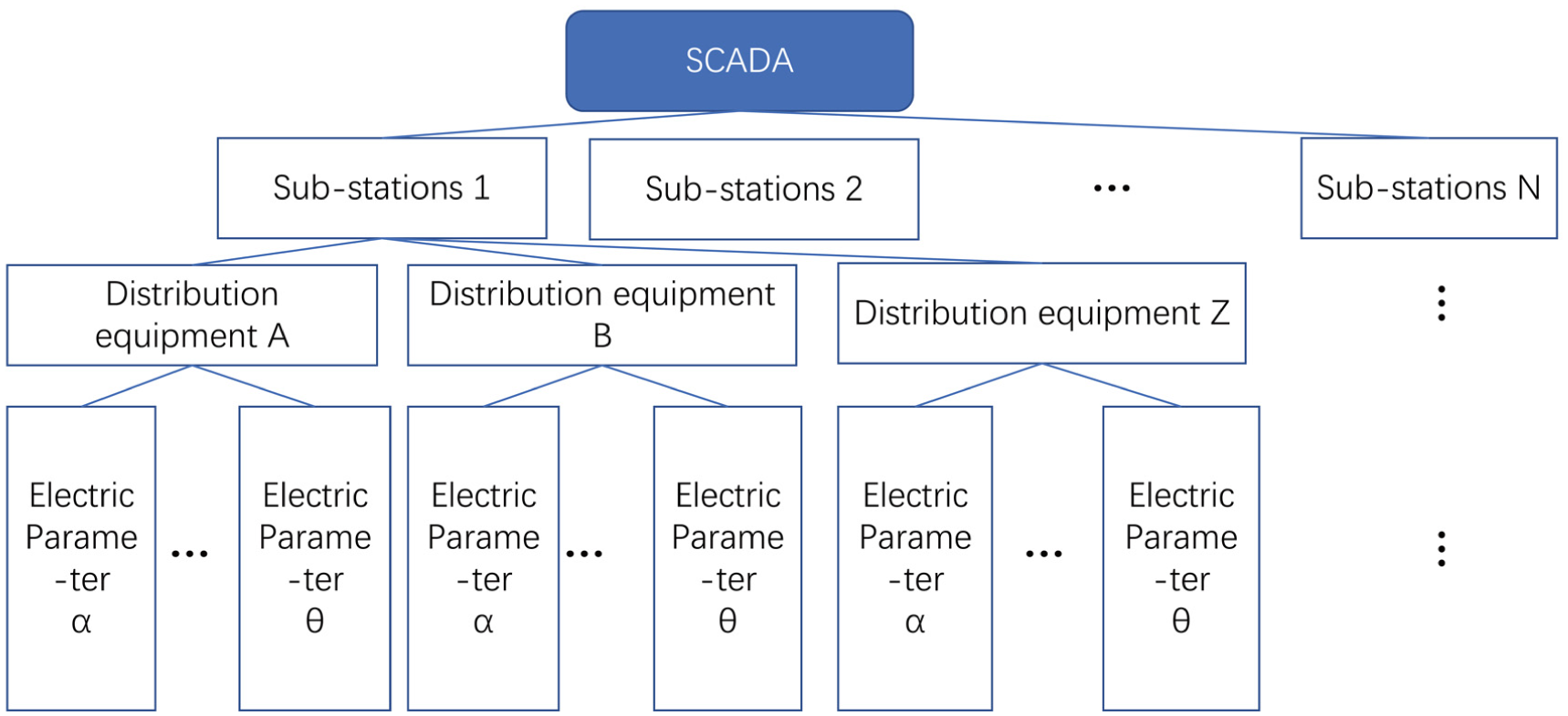
Electromechanical system structure of expressway bridges.

To transform the large volume of cluttered electrical data from expressway bridges into an informative matrix for further analysis, this paper applies standard data processing techniques to cluster and organize the data. The data from the same sub-station are clustered by distribution equipment or loop, and the parameters are arranged in the order of current, voltage, active power, reactive power, power factor, and frequency. Based on the interval arrangement characteristics of parameters and state data, the state matrix and parameter matrix are separated from the information matrix by circulation. The parameter matrix sorted by time step t is shown in Table 1.

Table 1.

Examples of Electrical Parameter Matrix of Expressway Bridge Electromechanical System

Data logging	t=0	t=1	t=2	t=3	t=4	t=5	t=6	t=7	t=8	t=9
NORTH_BRIDGE_MAINLINE.10kV_OL1_IA	0.333	0.000	0.000	0.000	0.667	0.333	0.000	0.000	0.667	0.333
NORTH_BRIDGE_MAINLINE.10kV_OL1_IB	0.667	0.000	0.000	0.333	0.667	0.333	0.000	0.333	1.000	1.000
NORTH_BRIDGE_MAINLINE.10kV_OL1_IC	0.000	0.000	0.667	0.333	0.333	0.000	0.000	0.000	0.333	0.333
NORTH_BRIDGE_MAINLINE.10kV_OL1_IAM	0.974	1.000	0.615	0.795	0.641	0.590	0.590	0.897	0.590	0.590
NORTH_BRIDGE_MAINLINE.10kV_OL1_IBM	1.000	0.917	0.750	0.896	0.813	0.750	0.729	0.854	0.542	0.479
NORTH_BRIDGE_MAINLINE.10kV_OL1_3U0	0.042	0.083	0.042	0.000	0.000	0.208	0.083	0.083	0.042	0.167
NORTH_BRIDGE_MAINLINE.LP8-1_SB_Ua	0.117	0.000	0.133	0.283	0.300	0.167	0.283	0.217	0.217	0.483
NORTH_BRIDGE_MAINLINE.LP8-1_SB_Ub	0.016	0.000	0.033	0.197	0.131	0.033	0.148	0.197	0.295	0.623
NORTH_BRIDGE_MAINLINE.LP8-1_SB_Uc	0.068	0.000	0.085	0.136	0.136	0.068	0.170	0.203	0.271	0.627
NORTH_BRIDGE_MAINLINE.LP8-1_SB_Uab	0.072	0.000	0.093	0.268	0.237	0.113	0.237	0.227	0.278	0.608

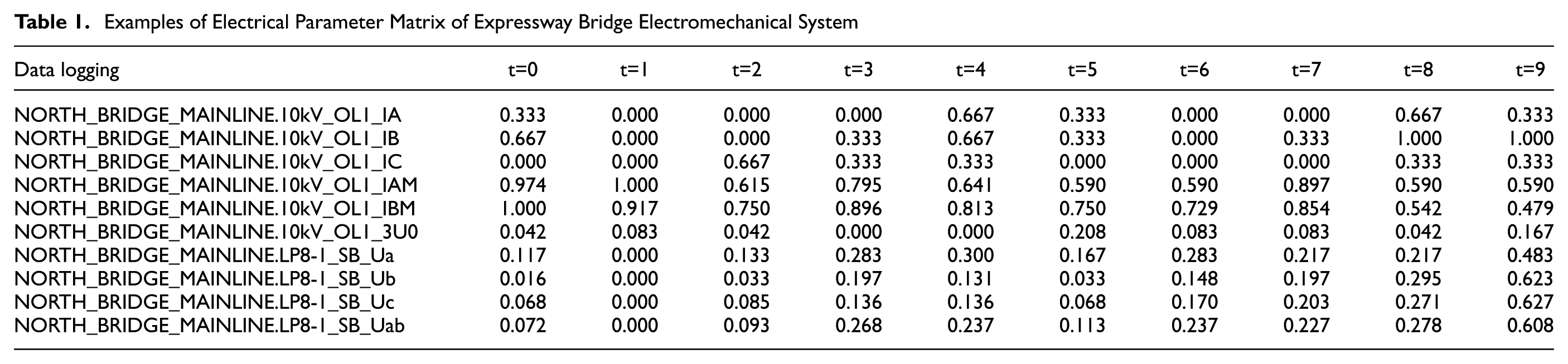
The state matrix consists of binary values (0 and 1), indicating whether each device is operating normally. The parameter matrix contains specific electrical quantities. Because of the wide fluctuation in value ranges, minimum-maximum normalization is used to map the values to a range of 0–1, and Z-score normalization is applied to standardize the data to a dimensionless set conforming to a normal distribution. Table 1 provides an example of the electrical parameter information matrix of the electromechanical system of an expressway bridge. Based on the characteristics of actual mechanical and electrical system fault maintenance records and electrical data, the reflected fault types are categorized into three main types:

Overcurrent (F = 0): Excessive use of electrical facilities leads to a sharp increase in the load on some lines in a short time, resulting in trip faults.

Equipment strain (F = 1): Trip faults caused by equipment defects or aging, line aging, and insulation performance degradation.

Other external failures (F = 2): Trip failures caused by thunderstorms, human-caused damage, and so forth, manifesting as short-term loss of electrical data and extremely high overvoltage caused by many bound charges.

Recurrent Neural Network for Fault Classification Model (RNN-FCM)

RNNs have demonstrated excellent performance in feature extraction from time series data. This section examines fault classification models for electromechanical systems based on three typical types of RNN. The proposed structure of a simple RNN for fault classification is illustrated in Figure 2 ( 23 ). Compared with the classical RNN structure, this study modifies the input and hidden layers in the simple RNN-FCM. A dense layer is added after the output layer, and a Softmax layer is used as the classifier for the feature vector, producing the confidence levels for each category. 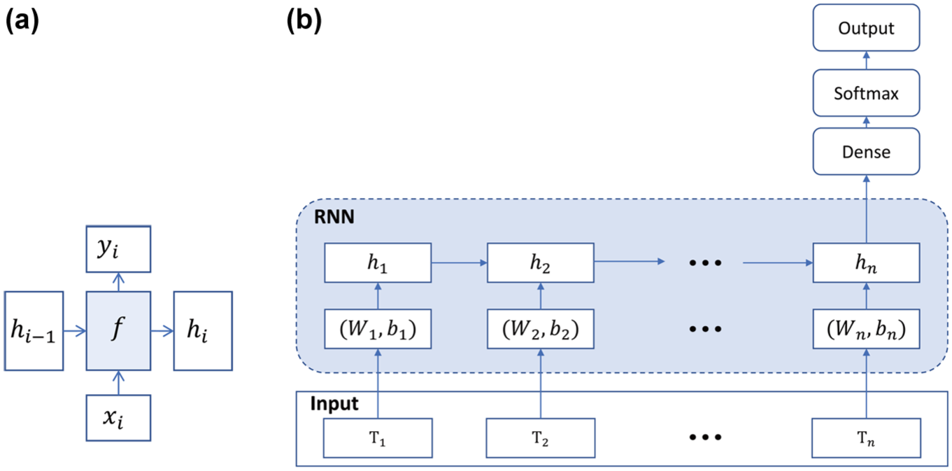As shown in Figure 2, the input $T_{i}$ with size $(X, t)$ is an electrical information matrix of the electromechanical system of the expressway bridge at each moment, where X is the total parameters of each sub-station and $t$ is time step. The hidden layer has a weight of $(W_{i}, b_{i})$ and a size of 64. The hidden state $h_{i}$ and the input $T_{i + 1}$ determine the output at $i + 1$ . $f$ is the activation function. $y_{n}$ is the output at the last point in time with size $(64, t)$ and is compressed into $(3, t)$ by the dense layer. Each dimension of the output vector represents the classification confidence to the information matrix at the input time t. The type of fault is classified by Softmax classifier.

Figure 2.

Recurrent neural network (RNN) for fault classification: (a) block construction and (b) RNN.Note:h_i = hidden state; f = activation function; x_i = station parameter; y_i = output feature; W_i = weight matrix; b_i = bias; T_i= input matrix.

Gated Recurrent Unit for Fault Classification Model (GRU-FCM)

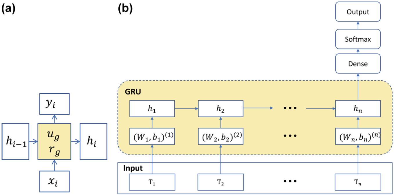
GRU, proposed in 2014, is a structure of RNN ( 24 ). The GRU-FCM of expressway bridges electromechanical systems is shown in Figure 3. Reset gate $r_{g}$ and update gate $u_{g}$ are used to control the update and transmission of hidden state $h_{i}$ in the block construction of GRU-FCM, as shown in Figure 3a. In Figure 3b, the input $T_{i}$ with size $(X, t)$ is the electrical information matrix at each moment, where $X$ is the total parameters of each sub-station. The weight of hidden layer is $(W_{i}, b_{i})$ whose size is 64. $y_{n}$ is the output at the last time point with size $(64, t)$ and is compressed into $(3, t)$ by the dense layer. Each dimension of the output vector represents the classification confidence to the information matrix at the input time $t$ . The type of fault is classified by Softmax classifier.

Figure 3.

Gated recurrent unit (GRU) for fault classification: (a) block construction and (b) GRU.Note: h_i = hidden state; u_g = update gate; r_g = reset gate; x_i = station parameter; y_i = output feature; W_i = weight matrix; b_i = bias; T_i = input matrix.

Long Short-Term Memory for Fault Classification Model (LSTM-FCM)

LSTM is a temporal RNN ( 25 ). The LSTM-FCM of expressway bridges’ electromechanical systems is shown in Figure 4. Input gate i_g, forgetting gate f_g, and output gate O_g to control the update and transmission of hidden state h_i and kernel state c_i in the block construction of LSTM-FCM, as shown in Figure 4a. In Figure 4b, the input layer and hidden layer of LSTM-FCM are adjusted. The input T_i with size (X,t) is the electrical information matrix at each moment, where X is the total parameters of each sub-station. The weight of hidden layer (W_i,b_i) is whose size is 64. y_n is the output at the last time point with size (64,t) and is compressed into (3,t) by the dense layer. Each dimension of the output vector represents the classification confidence to the information matrix at the input time t. The type of fault is classified by Softmax classifier.

Figure 4.

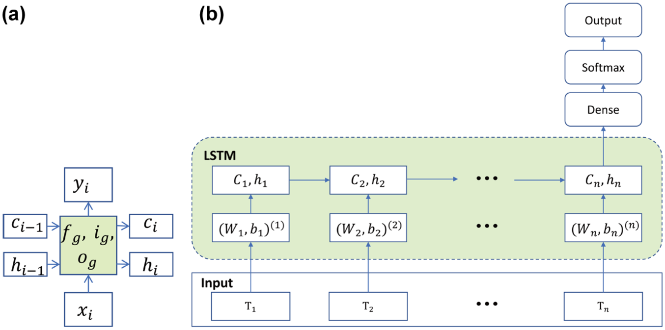
Long short-term memory (LSTM) for fault classification: (a) block construction and (b) LSTM.Note:h_i = hidden state; c_i = cell state; i_g = input gate; o_g = output gate; f_g = forgetting gate; x_i = station parameter; y_i = output feature; W_i = weight matrix; b_i = bias; T_i = input matrix.

The process of real-time classification of electromechanical systems fault states of expressway bridges by RNN-FCM, GRU-FCM and LSTM-FCM is as follows:

$x$ is the time series of the electrical parameter information matrix of the expressway electromechanical system, as the input of the model, while $y$ is the output. $m$ is the number of samples. Thus, the training set is:

{(x_{1}, y_{1}), (x_{2}, y_{2}), \dots, (x_{m}, y_{m})}, y \in {0, 1, 2}

(1)

2) Data features are extracted, added, and diminished layer-by-layer until the last moment through the recurrent unit of RNN-FCM, GRU-FCM, and LSTM-FCM. $z_{i}$ are output after the dense layer, and are classified in Softmax classifier. Softmax classifier is an extension of the logistic regression model on multiple classification problems. Let $k$ be the number of fault classes, and the output probability of the fault classes is:

{\hat{y}}_{i} = softmax (z_{i}) = \frac{z_{i}}{\sum_{j = 1}^{k} z_{j}}

(2)

3) According to maximum likelihood estimation, the loss function is shown in Equation 3. The network is trained iteratively using gradient descent to update the parameters and minimize the loss function.

L = - \sum_{i = 1}^{k} y_{i} \log ({\hat{y}}_{i})

(3)

Fused Stack Sparse Long Short-Term Memory (FSS-LSTM) Network for Fault Classification of Expressway Bridge Electromechanical System

To improve the classification efficiency and learning ability of discrete data, this paper proposes a sparse connection and stack structure for LSTM, inspired by the stacked sparse auto-encoder ( 26 ). Sparse connection involves adding sparsity constraints between two layers, so that some nodes participate in parameter transmission and calculation, while others are suppressed, as shown in Figure 5b. Compared with the full connection in Figure 5a, sparse connection can learn super-complete vectors to represent the input features. The method of implementing the sparsity constraint is as follows. The sigmoid function is set as the activation function for the hidden layer, with a value range of [0, 1]. In this context, a value of 1 indicates that the node is active, while a value of 0 indicates that the node is inactive. To measure the relationship between the average activation output of hidden layer nodes and the desired sparsity ρ, Kullback-Leibler (KL) divergence is introduced:

KL (ρ | | \hat{ρ}) = ρ \log \frac{ρ}{{\hat{p}}_{j}} + (1 - ρ) \log \frac{1 - ρ}{1 - {\hat{p}}_{j}}

(4)

where

${\hat{p}}_{j} = \frac{1}{m} \sum_{i = 1}^{m} [a_{j}^{(2)} x^{(i)}]$ = the average activation value of the hidden node $j$ in the training set,

$m$ = the number of training samples, and

$a_{j}^{(2)} x^{(i)}$ = the activation value output of the node $j$ to sample $i$ .

Generally, $ρ$ is set as 0.05 or 0.1.

Sparse constraint is achieved by adding KL into the loss function as a regular term:

J_{sparse} (W, b) = J (W, b) + β \sum_{j = 1}^{s} KL (ρ | | \hat{ρ})

(5)

where

J = the loss function,

W = the weight of the network,

b = the bias term,

$β$ = the weight of the sparse constraint term, and

s = the number of nodes in the hidden layer.

Figure 5.

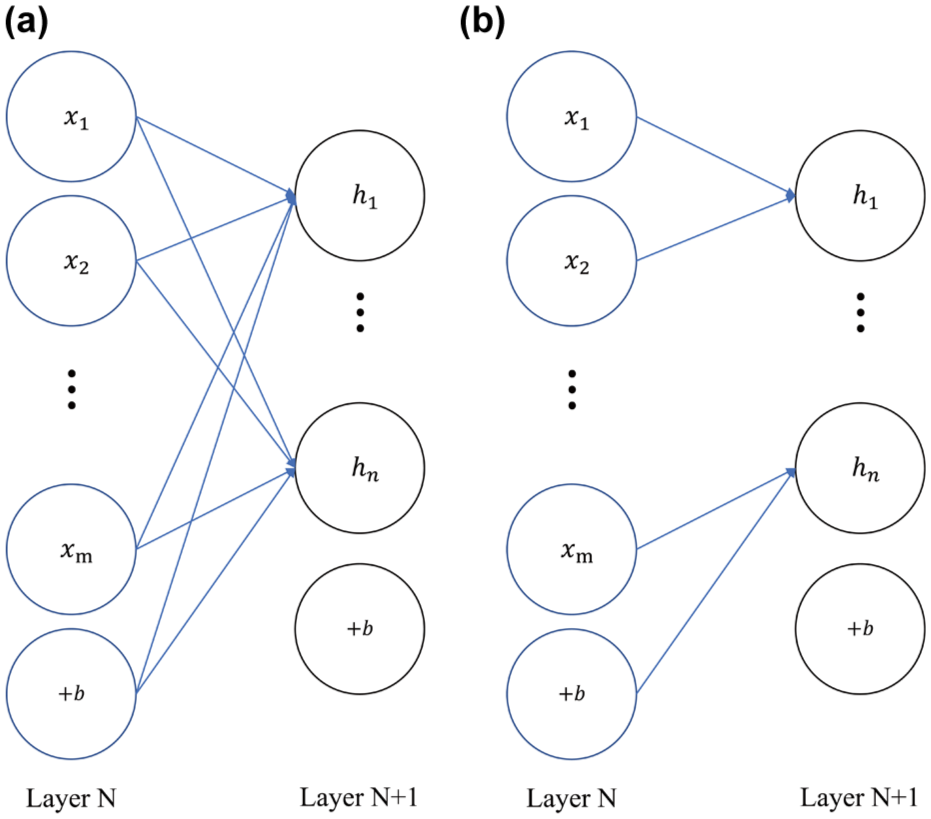
Structures of: (a) full connection and (b) sparse connection.Note:xi = Layer N neuron; hi = Layer N+1 neuron; bi = bias.

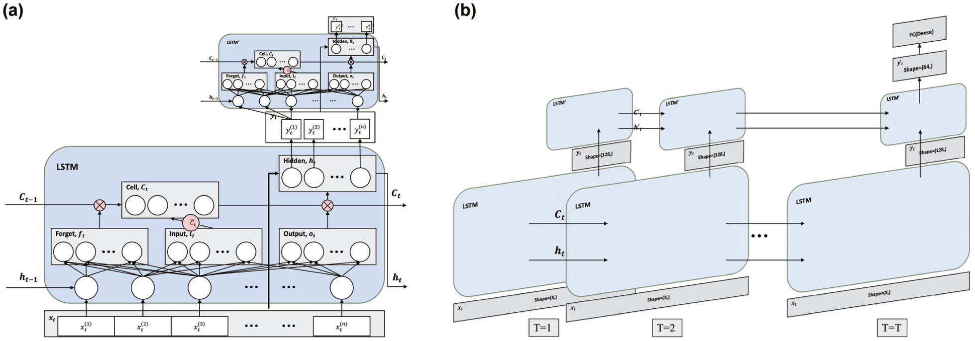
Figure 6a details the single computing unit of the FSS-LSTM network at time t. The entire structure of the FSS-LSTM network is shown in Figure 6b. Compared with conventional LSTM, the FSS-LSTM network increases computing layers and incorporates sparsity. The output feature vectors of the single computing unit $y_{t}^{(n)}$ are used as the input of deep hidden layers, where all output features at time t are fused with sparse connection. The first hidden layer returns the output of all nodes, while the second hidden layer returns the output of the last node. Specifically, the sparse weight KL, with an initial value of 0.5, is used to enforce sparse connections. By adding an activity regularizer to the first hidden layer, the second hidden layer obtains sparse features.

Figure 6.

Structure of fused stack sparse long short-term memory (FSS-LSTM) networks for fault classification of expressway electromechanical systems: (a) single computing cell unit and (b) network structure in time dimension.Note:h_t = hidden state; c_t = cell state; i_g = input gate; o_g = output gate; f_g = forgetting gate; x_t = station parameter; y_t = output feature; W_i = weight matrix; b_i = bias; t = time dimension.

The specific working process of the FSS-LSTM network is as follows:

In a single operation unit of the FSS-LSTM network, the input has a size of (x,t), where x is the parameter size of the electrical information matrix, and t is the time dimension. Feature calculation and extraction are carried out by the forget gate, input gate, and output gate, respectively. The first hidden layer of the FSS-LSTM has a size of 128, so the output has a size of (128,t). This hidden layer extracts features from the input parameter matrix, which are compressed into a low-dimensional vector with size 128 by the recurrent units. The output features are passed upward at each time step t.

The first hidden layer and the second hidden layer of the FSS-LSTM network are connected by a sparse weight with an initial value of 0.5. The input size of the second hidden layer is (128,t), and the computational dimension is 64. Each time node passes the kernel state and hidden state to the next node but does not output features upward.

The output at time t with a size of (64,t) enters the fully connected layer of the FSS-LSTM network, which compresses the 64-dimensional features into 3-dimensional features. The output size of the entire model is (3,t), representing the corresponding classification confidence at each time step t.

The proposed FSS-LSTM network can classify electromechanical system faults of expressway bridges in real time. For example, when t = 1, the input vector has a size of (x,1) and the output dimension of the first layer is (128,1), which can be considered a one-dimensional vector. The output dimension of the second layer is (64,1), representing the output feature of a single moment. After processing through a fully connected layer and a Softmax classifier, a 3-dimensional vector is output as the classification result.

Experiments

In this section, we conducted experiments to evaluate the performance of the aforementioned neural networks for fault classification using the SEU Electromechanical System Dataset. This dataset was collected from the SCADA system of the Taizhou Yangtze River Bridge electromechanical system, a large-span bridge across the Yangtze River in China, with a two-way six-lane expressway. The bridge comprises 13 sub-stations: North_Bridge_Mainline, Gao_Gang, North_Anchor, North_Tower, Central_Tower, South_Tower, South_Anchor, Yang_Zhong, South_Bridge_Mainline, Yao_Bridge, New_Bridge, Xiao_Huang_Shan_Service_Area, and Meng_He. The fault types were determined by collecting and analyzing the electrical time sequence data. The data was collected from January 1, 2017, to December 30, 2020, totaling 36,150 h. The electromechanical system generates electrical data logs every hour, resulting in 36,150 sampling points in the time series. The feature dimension for the experiments in this paper is 800, although other electromechanical systems may have different feature dimensions based on specific conditions. The number of fault samples (hours) for each sub-station are as follows: 1,039, 210, 156, 1,178, 141, 147, 302, 326, 304, 283, 452, 374, and 493, respectively. Based on the maintenance records of the Taizhou Yangtze River Bridge expressway’s electromechanical system, the failure types are categorized into overload (F = 0), equipment strain (F = 1), and other external failures (F = 2). The total number of fault samples is 6,081, with 3,117 samples for overcurrent, 907 samples for equipment strain, and 1,715 samples for other external failures. The data from m time steps before the fault occurrence is used to form an electrical parameter matrix as the fault sample. For instance, if m = 150, the dimension of a fault sample is (150,800).

The following experiments were conducted using Jupyter Notebook (Ipython) with Python 3.6 and Keras 2.1 deep-learning packages (TensorFlow as the backend), and relied on modules such as Pandas 1.1.5, Numpy 1.19, and Matplotlib 3.3. The computer used for the experiments was configured with an Intel(R) Core™ i7-10710 CPU @ 1.10 GHz (1.61 GHz) and 32 GB of RAM.

Comparative Experiments of RNN-FCM, GRU-FCM and LSTM-FCM Networks

To analyze the adaptability and convergence of the RNN-FCM, LSTM-FCM, and GRU-FCM networks with different optimizers, this study selected stochastic gradient descent (SGD), Adam, and Nadam for the experiments. Figure 7 shows the convergence curves of the RNN-FCM network with different optimizers, where Figure 7a illustrates the changes in training loss over time, and Figure 7b shows the validation loss. As depicted in Figure 7, the convergence curves of SGD declined more slowly than those of the other two optimizers, exhibiting significant fluctuations within the first 12 training epochs, and finally converging at the 20th epoch. The validation loss of SGD was notably higher than that of Adam and Nadam. The training loss and validation loss for the Adam and Nadam optimizers are approximately the same on the final convergence curve, but Nadam requires more time to converge.

Figure 7.

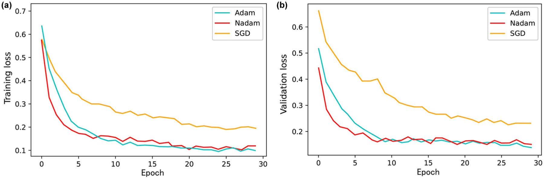
Convergence curves of recurrent neural network for fault classification model (RNN-FCM) using optimizer of stochastic gradient descent (SGD), Adam, and Nadam: (a) train_loss and (b) validation_loss.

The training accuracy of the SGD, Adam, and Nadam optimizers for the RNN-FCM, LSTM-FCM, and GRU-FCM networks is shown in Table 2. GRU-FCM performs well on the training set but worse than LSTM-FCM on the validation set, indicating that GRU-FCM is overfitting. LSTM-FCM achieves higher validation accuracy when using the Adam optimizer, reaching 95.8% on the training set and 88.8% on the validation set. To test the stability and robustness of the RNN-FCM, GRU-FCM, and LSTM-FCM networks, 100 time series sampling experiments were performed using the SEU Electromechanical System Dataset. In each experiment, 20% of the data samples were randomly selected, with the first 60% as the training set, the middle 20% as the validation set, and the remaining 20% as the test set. The average test accuracy of the RNN-FCM, GRU-FCM, and LSTM-FCM networks was calculated. The results of the cross-validation experiments are shown in Figure 8. In Figure 8a, the accuracy of LSTM-FCM reaches 89.73%, outperforming the RNN-FCM and GRU-FCM networks. As shown in Figure 8b, the box plot of the LSTM-FCM network has a smaller distribution span and a higher average accuracy than the other two models.

Table 2.

Accuracy Comparison of Recurrent Neural Network Fault Classification Model (RNN-FCM), Gated Recurrent Unit Fault Classification Model (GRU-FCM), and Long Short-Term Memory Fault Classification Model (LSTM-FCM)

Model	Optimizer = SGD		Optimizer = Adam		Optimizer = Nadam
Model	train-acc	val-acc	train-acc	val-acc	train-acc	val-acc
RNN-FCM	0.803	0.840	0.830	0.824	0.830	0.822
GRU-FCM	0.982	0.768	0.967	0.852	0.957	0.842
LSTM-FCM	0.943	0.783	0.948	0.888	0.958	0.888

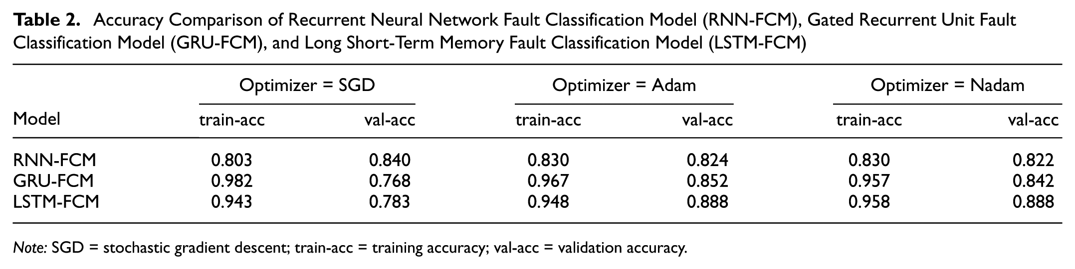
Note: SGD = stochastic gradient descent; train-acc = training accuracy; val-acc = validation accuracy.

Figure 8.

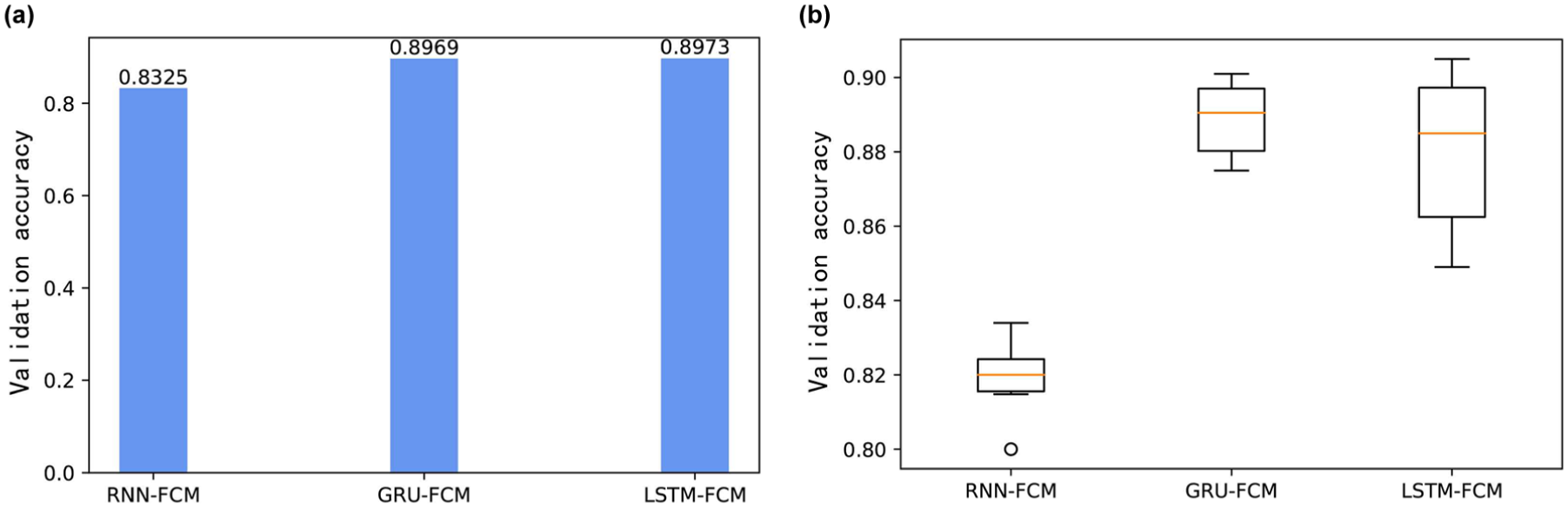
Cross validation accuracy comparison of recurrent neural network fault classification model (RNN-FCM), gated recurrent unit fault classification model (GRU-FCM), and long short-term memory fault classification model (LSTM-FCM): (a) bar plots of classification rates and (b) box plots of classification rates.

Comparative Experiments of FSS-LSTM and Other Networks

All experiments were implemented on a PyTorch framework with an NVIDIA GPU. The sequence length was set to 64 (matching the sampling interval and temporal resolution of SCADA monitoring data); batch size was fixed at 32. The optimizers were adopted with an initial learning rate of 1 × 10⁻³, momentum parameters β₁ = 0.9, β₂ = 0.999, and no learning rate decay during training. The model was trained for 100 epochs with an early-stop patience of 10 epochs to avoid overfitting. For the FSS-LSTM structure: the hidden dimension of each LSTM layer was 128, a dropout rate of 0.2 was applied between hidden layers, and the sparse constraint coefficient was set to 0.5 to balance feature sparsity and classification performance.

To analyze the adaptability and convergence of the FSS-LSTM network with different optimizers, this experiment applied both the Adam optimizer and the Nadam optimizer to train the FSS-LSTM for 15 epochs with a batch size of 64. The training process of the FSS-LSTM model using the Adam and Nadam optimizers is shown in Figure 9. The training curves for both optimizers are similar, but the validation loss for the Nadam optimizer fluctuates significantly. After 15 epochs, the validation loss for the Adam optimizer increases slightly, indicating potential overfitting. Regardless of whether the Adam or Nadam optimizer is used, the training accuracy and validation accuracy of the FSS-LSTM network can reach 96% and 93%, respectively. However, the convergence curve for the Adam optimizer is more stable.

Figure 9.

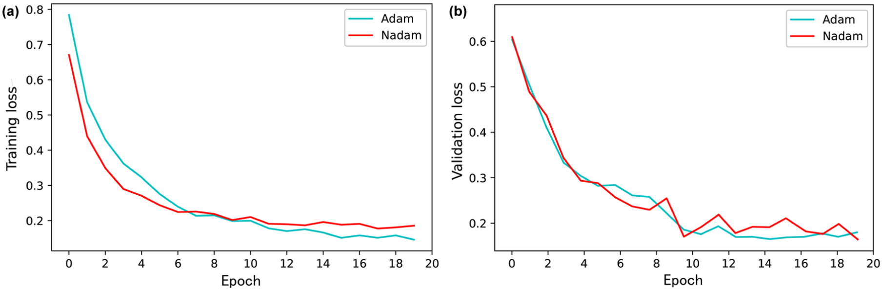
Convergence curves of fused stack sparse long short-term memory (FSS-LSTM) using Adam and Nadam optimizers: (a) train_loss and (b) validation_loss.

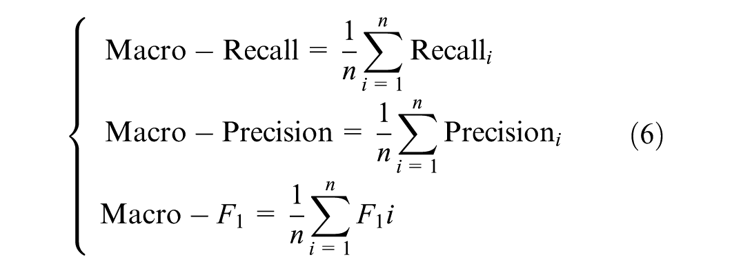
The performance advantages of the FSS-LSTM network were verified through contrast experiments. The failures included overload (F = 0), equipment strain (F = 1), and other external faults (F = 2). Twenty percent of the dataset was used for testing. The total number of failed nodes (hours) per substation test sample was 212, 34, 28, 250, 25, 28, 66, 61, 60, 55, 98, 61, and 109, respectively. Generally, the experimental dataset is not shuffled. However, because the fault samples of some substations are unevenly distributed over time, we divided the dataset into two or three blocks to ensure that the test set includes all three fault types while maintaining the order of samples within each block. Blocks were not allowed to overlap to avoid data leakage. Given the data imbalance, a macro-average was used to evaluate model performance, as shown in Equation 6.

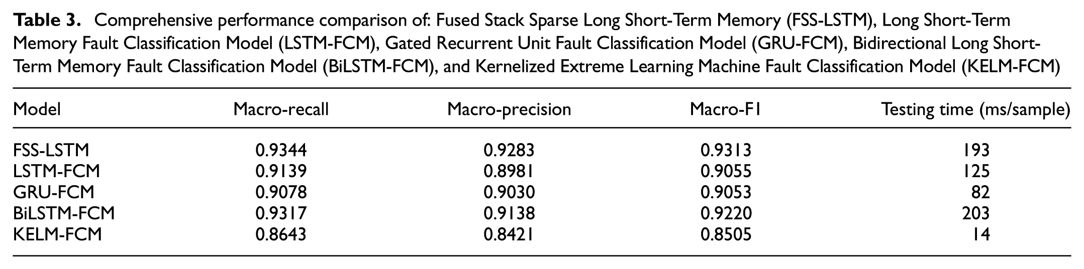
{\begin{matrix} Macro - Recall = \frac{1}{n} \sum_{i = 1}^{n} Recal l_{i} \\ Macro - Precision = \frac{1}{n} \sum_{i = 1}^{n} Precisio n_{i} \\ Macro - F_{1} = \frac{1}{n} \sum_{i = 1}^{n} F_{i} \end{matrix}

(6)

As shown in Table 3 and Figure 10, the comprehensive performance of the FSS-LSTM network is superior to the other four models, with macro-recall, macro-precision, and macro-F1 reaching 0.9400, 0.9348, and 0.9371, respectively. In time consumption, FSS-LSTM takes longer because of the increased computational complexity and test time resulting from the depth and sparsity of the network, but it is still faster than BiLSTM-FCM.Compared with the other four models, the box plot of FSS-LSTM shows a smaller distribution span and a higher average value, indicating greater stability.

Table 3.

Comprehensive performance comparison of: Fused Stack Sparse Long Short-Term Memory (FSS-LSTM), Long Short-Term Memory Fault Classification Model (LSTM-FCM), Gated Recurrent Unit Fault Classification Model (GRU-FCM), Bidirectional Long Short-Term Memory Fault Classification Model (BiLSTM-FCM), and Kernelized Extreme Learning Machine Fault Classification Model (KELM-FCM)

Model	Macro-recall	Macro-precision	Macro-F1	Testing time (ms/sample)
FSS-LSTM	0.9344	0.9283	0.9313	193
LSTM-FCM	0.9139	0.8981	0.9055	125
GRU-FCM	0.9078	0.9030	0.9053	82
BiLSTM-FCM	0.9317	0.9138	0.9220	203
KELM-FCM	0.8643	0.8421	0.8505	14

Figure 10.

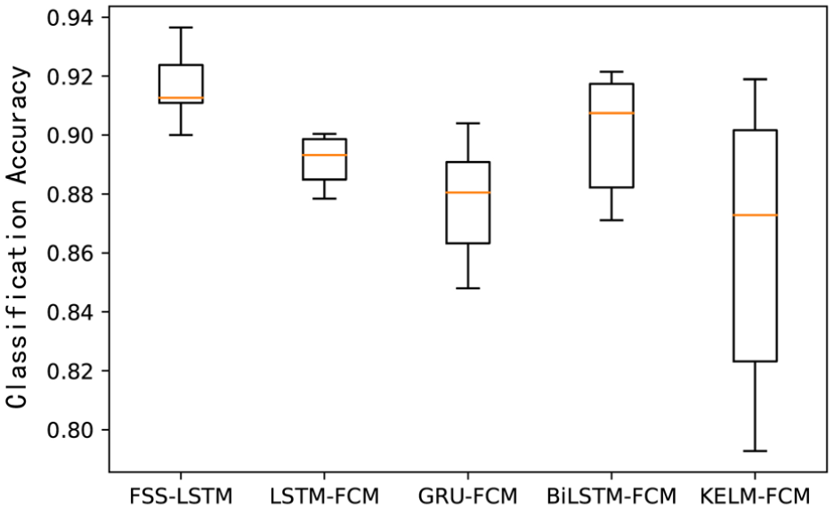
Box plots of classification accuracy of fused stack sparse long short-term memory (FSS-LSTM), gated recurrent unit fault classification model (GRU-FCM), long short-term memory fault classification model (LSTM-FCM), bidirectional long short-term memory fault classification model (BiLSTM-FCM), and kernelized extreme learning machine (KELM).

The comparison of F1 scores for the five networks is shown in Figure 11. When F = 0, FSS-LSTM has the highest F1 score, mainly because faults classified as F = 0 are caused by an increased load on the line, which is characterized by a sharp increase in electrical parameters. When F = 1, the F1 score of FSS-LSTM is relatively low, mainly because the transient fluctuation characteristics of electrical data caused by equipment strain are not significant. The F1 scores of FSS-LSTM, LSTM-FCM, GRU-FCM, and BiLSTM-FCM show little difference in this case. For F = 2, which represents other external faults often manifested as damage to individual devices, FSS-LSTM and BiLSTM-FCM significantly outperform LSTM-FCM and GRU-FCM in F1 score. This indicates that the increased complexity of the model improves its ability to capture local feature changes effectively.

Figure 11.

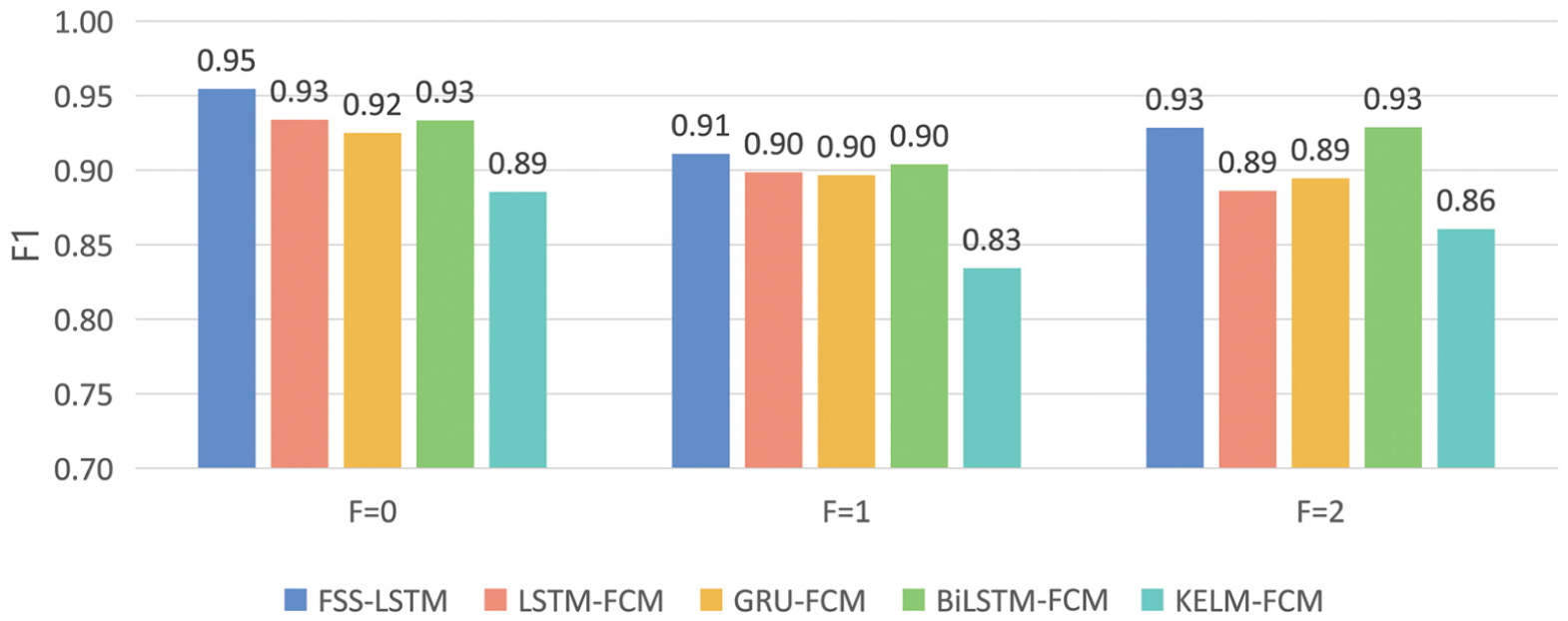
Comparison of F1 score of fused stack sparse long short-term memory (FSS-LSTM), gated recurrent unit fault classification model (GRU-FCM), long short-term memory fault classification model (LSTM-FCM), bidirectional long short-term memory Fault Classification Model (BiLSTM-FCM), and Kernelized Extreme Learning Machine Fault Classification Model (KELM-FCM): F = 0 (overcurrent), F = 1 (strain), and F = 2 (other external failures).

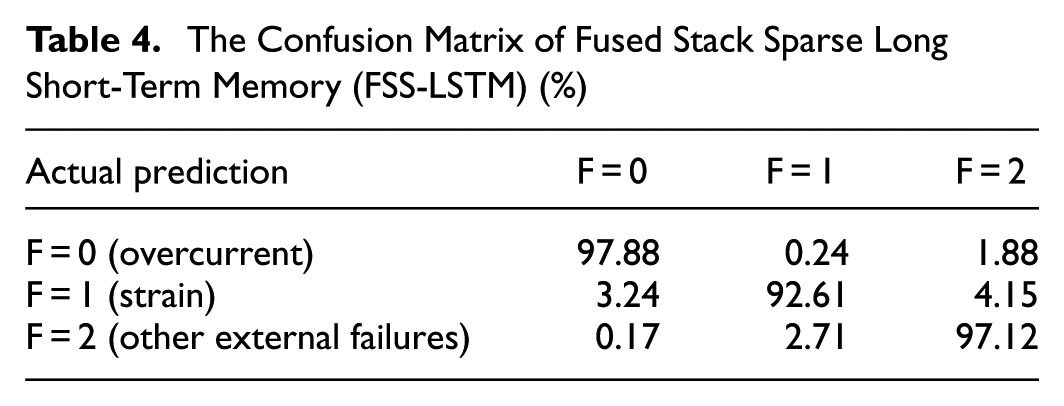
Table 4 shows the confusion matrix of the FSS-LSTM. Each row represents the actual category, and each column represents the predicted category. Individual classification accuracy values are calculated for all fault types. The classificaiton accuracy of fault label F = 0 is 97.88%. F = 1 has an accuracy of 92.61%, and F = 2 reaches 97.12%. The highest accuracy is observed for F = 0, mainly because faults classified as F = 0 are caused by an increased load on the line, which is characterized by a sharp increase in electrical parameters. The classification accuracy for F = 1 is relatively lower, primarily because the transient fluctuations in electrical data caused by equipment strain do not exhibit significant characteristic changes.

Table 4.

The Confusion Matrix of Fused Stack Sparse Long Short-Term Memory (FSS-LSTM) (%)

Actual prediction	F = 0	F = 1	F = 2
F = 0 (overcurrent)	97.88	0.24	1.88
F = 1 (strain)	3.24	92.61	4.15
F = 2 (other external failures)	0.17	2.71	97.12

Conclusion

This paper develops an FSS-LSTM network for accurate and robust fault classification of electromechanical systems. First, SCADA data are utilized to construct an electrical information matrix, enabling the identification of complex and diversified operating states of the target electromechanical system. Second, the novel FSS-LSTM architecture is proposed by integrating sparsity constraints and temporal output fusion into a multi-layer LSTM framework, with performance comparisons conducted against GRU-FCM, LSTM-FCM, BiLSTM-FCM, and KELM-FCM models. Finally, comparative experiments are performed using SCADA data derived from the electromechanical centralized control system of the Taizhou Yangtze River Bridge.

Experiment results validate that the proposed FSS-LSTM network achieves superior fault classification performance for highway electromechanical systems over the four benchmark models. The electrical data employed are collected from the full substation, covering faults of distribution lines and equipment while excluding specific electromechanical equipment faults. The deployment of intelligent electromechanical fault classification can improve operational efficiency and reduce safety risks to highway operations caused by system failures.

This method enables proactive maintenance and early anomaly identification, which effectively reduces unexpected downtime and extends the service life of key electromechanical equipment. It also provides a reliable data-driven decision-making basis for the daily operation and maintenance of large-scale transportation infrastructure.

Notably, the imbalanced distribution of fault samples restricts the model’s recognition accuracy for minority fault categories. Despite satisfactory macro-average metrics, enhancing the classification accuracy of minority classes is critical for electromechanical maintenance. Additionally, targeted strategies, including optimized time-series sampling techniques and cost-sensitive learning, will be explored to alleviate the data imbalance issue in the future.

Footnotes

Acknowledgements

The authors would like to thank the Transportation Technology Project of Shaanxi Province. Their assistance is gratefully acknowledged.

Author Contributions

The authors confirm contribution to the paper as follows: Methodology, Formal analysis, Resources, Writing – original draft: Yang Liu; Conceptualization, Funding acquisition, Supervision, Writing – review & editing: Chihang Zhao; Data curation, Investigation, Validation: Zichen Qian. All authors reviewed the results and approved the final version of the manuscript.

Declaration of Conflicting Interests

The authors declared no potential conflicts of interest with respect to the research, authorship, and/or publication of this article.

Funding

The authors disclosed receipt of the following financial support for the research, authorship, and/or publication of this article: this article was supported by the Transportation Technology Project of Shaanxi Province (Grant No. 23-09X).

ORCID iDs

Yang Liu

Chihang Zhao

Zichen Qian

References

Zhao

Effect of Temperature and Humidity on Electrical Automation Equipment. Architectural Engineering Technology Design, Vol. 278, No. 1, 2015, pp. 1412–1419.

Malik

Mishra

Application of Gene Expression Programming (GEP) In Power Transformers Fault Diagnosis Using DGA. IEEE Transactions on Industry Applications, Vol. 52, No. 6, 2016, pp. 4556–4565.

Chellamuthu

Sekaran

E. C.

Fault Detection in Electrical Equipment’s Images by Using Optimal Features with Deep Learning Classifier. Multimedia Tools and Applications, Vol. 78, No. 19, 2019, pp. 27333–27350.

Qin

Liu

Ren

A Panel Data Model-Based Multi-Factor Predictive Model Of Highway Electromechanical Equipment Faults. IEEE Transactions on Intelligent Transportation Systems, Vol. 19, No. 9, 2018, pp. 3039–3045.

Chen

Gao

Using the Motor Power and XGBOOST to Diagnose Working States of a Sucker Rod Pump. Journal of Petroleum Science and Engineering, Vol. 199, 2021, pp. 108329.

Iman

Mourad

Ilias

Dahi

Multi-Source Information Fusion Fault Diagnosis for Rotating Machinery using Signal and Data Processing. Surveillance, Vibrations, Shock and Noise, Vol. 6, 2023, pp. 1–12.

Venkata

Pandya

, K. Vala,and A. V. Sant. Support Vector Machine for Fast Fault Detection and Classification in Modern Power Systems Using Quarter Cycle Data. Energy Reports, Vol. 8, 2022, pp. 92–98.

Xianwen

Xiangyu

Using the Motor Power and XGBOOST to Diagnose Working States of a Sucker Rod Pump. Journal of Petroleum Science & Engineering, Vol. 199, 2021, pp. 108329.

Zhang

Bahrampour

Ramakrishnan

Schott

Shah

Deep Learning on Symbolic Representations for Large-Scale Heterogeneous Time-Series Event Prediction. In 2017 IEEE International Conference on Acoustics, New Orleans, USA, 2017, pp. 5970–5974.

10.

Grüner

Böllhoff

Meisetschläger

Vydrenko

Bator

Dicks

Theissler

Evaluation of Machine Learning for Sensorless Detection and Classification of Faults in Electromechanical Drive Systems. Procedia Computer Science, Vol. 176, 2020, pp. 1586–1595.

11.

Tefera

Y. Y.

Kibatu

Shawel

B. S.

Woldegebreal. Recurrent Neural Network-Based Base Transceiver Station Power Supply System Failure Prediction. In 2020 International Joint Conference on Neural Networks, Glasgow, UK, 2020, pp. 1–7.

12.

Cenek

Haro

Sayers

Peng

Climate Change and Power Security: Power Load Prediction for Rural Electrical Microgrids Using Long Short Term Memory and Artificial Neural Networks. Applied Sciences, Vol. 8, No. 5, 2018, pp. 749–765.

13.

Kong

Dong

Z. Y.

Jia

Hill

D. J.

Zhang

Short-Term Residential Load Forecasting Based on LSTM Recurrent Neural Network. IEEE Transactions on Smart Grid, Vol. 10, No. 1, 2017, pp. 841–851.

14.

Georgoulopoulos

Hatzopoulos

Karamitsios

Tabakis

I. M.

Kotrotsios

Metsai. A Survey on Hardware Failure Prediction of Servers Using Machine Learning and Deep Learning. In 2021 International Conference on Modern Circuits and Systems Technologies, Thessaloniki, Greece, 2021, pp. 1–5.

15.

Zhang

Cao

Yang

Sun

Wang

Motor Current Signal Analysis Using Hypergraph Neural Networks for Fault Diagnosis of Electromechanical System. SSRN Electronic Journal, Vol. 8, 2022, pp. 1–8.

16.

Luo

Cheng

Deng

Sun

Liu

Incipient Fault Detection In Power Distribution System: A Time–Frequency Embedded Deep-Learning-Based Approach. IEEE Transactions on Instrumentation and Measurement, Vol. 72, 2023, pp. 1–14.

17.

Tian

Wei

Zhu

Intelligent Fault Diagnosis in Power Distribution Networks Using LSTM-Densenet Network. Electric Power Systems Research, Vol. 2, 2025, pp. 239.

18.

Wei

Jiao

Fault Status Information Monitoring Technology for Large Complex Electromechanical System. Jordan Journal of Mechanical & Industrial Engineering, Vol. 15No. 1, 2021, pp. 105–112.

19.

Zhao

Huo

Cui

Design of Fault Diagnosis Algorithm for Electromechanical System Based on Artificial Intelligence. Journal of Physics: Conference Series. Vol. 2025, No. 1, 2021,p. 012011.

20.

Ayodeji

Mujeeb

A. A.

Defining Accuracy Benchmarks for Freeway Traffic Simulations in Support of Highway Operations and Planning. World Journal of Advanced Research and Reviews, Vol. 27, No. 02, 2025, pp. 790–797

21.

Mujeeb

A. A.

Wei

A Priority Based Multi-Level Heterogeneity Modelling Framework for Vulnerable Road Users. Transportmetrica A: Transport Science, Vol. 21, 2025, pp. 1–34.

22.

Zhu

Lei

Chai

Mazur

Huang

A Review of The Application of Deep Learning in Intelligent Fault Diagnosis of Rotating Machinery. Measurement, Vol. 206, 2023, p. 24.

23.

Fekri

M. N.

Patel

Grolinger

Sharma

Deep Learning for Load Forecasting with Smart Meter Data: Online Adaptive Recurrent Neural Network. Applied Energy, Vol. 282, 2021, p. 116177.

24.

Wei

Zhang

Yang

H. Q.

Zhang

Yao. Machine Learning for Pore-Water Pressure Time-Series Prediction. Geoscience Frontiers, Vol. 12, No. 1, 2021, pp. 453–467.

25.

Sherstinsky

Fundamentals of Recurrent Neural Network (RNN) and Long Short-Term Memory (LSTM) Network. Physica D: Nonlinear Phenomena, Vol. 404, 2020, p. 132306.

26.

Wang

Quan

Song

Lei

and Structural Sparsity Auto-Encoder with L21-Norm Minimization. Neurocomputing, Vol. 425, No. 2, 2021, pp. 71–81.