Estimating Percentile Speeds with Probe Vehicle Data on Non-Freeways

Abstract

Accurate estimation of percentile operating speeds on arterial roads is crucial for calibrating crash-prediction models, evaluating eligibility conditions for traffic safety countermeasures, and informing speed-management decisions. Existing percentile-speed estimation models were developed for specific regions, so their transferability to other geographical jurisdictions needs to be evaluated. To fill this gap, this study develops and validates an 85th-percentile speed (V₈₅) model for non-freeway arterials using probe vehicles, field surveys, and roadway data. A dataset comprising sixty spot-speed surveys (forty-two urban and eighteen rural) collected in Maryland from 2019 to 2025 was matched to corresponding INRIX segment speeds, roadway geometric attributes, and traffic volumes. Ordinary-least-squares regression analyses were conducted for urban and rural settings, incorporating key variables including INRIX segment speed, posted speed limit, directional annual average daily traffic, segment length, lane width, access density, signal density, and functional-class indicators. The proposed model demonstrated high predictive accuracy for both urban and rural segments, achieving substantial error reductions compared with the baseline Texas A&M Transportation Institute model and a locally calibrated model. The findings also show that the posted speed limit is essential in rural V₈₅ estimation and remains useful in urban contexts. The model also supports network screening for segments that may warrant speed management or safety review.

Keywords

85th percentile speed operating speed estimation probe vehicle data speed screening

Introduction

Traffic speed is one of the most readily observed reflections of how drivers perceive and respond to their roadway environment. Among the available operating-speed metrics, the 85th percentile speed (V₈₅) plays an important role. It is fundamental to many applications, including the setting of appropriate speed limits ( 1 ), conducting crash and safety analyses, and designing effective traffic-calming strategies. Accurate estimation of V₈₅ enables transportation agencies to make informed decisions aimed at enhancing roadway safety, efficiency, and overall traffic management.

Traditional methods for estimating V₈₅ typically rely on direct field measurements. Although effective, these methods are often costly, time-consuming, and logistically challenging, especially when covering large roadway segments. Thus, there is a need for alternative, efficient modeling approaches that can reliably estimate V₈₅ using readily available data sources. Existing models, such as the Texas A&M Transportation Institute (TTI) percentile speed estimation model (11), have been developed and calibrated primarily within specific geographic contexts. Despite these developments, their effectiveness and accuracy when applied to different regions remain unclear, indicating a gap in understanding the transferability of such models—particularly in contexts with varied road characteristics and regional driving behaviors.

The objective of this study is to evaluate the applicability of an existing percentile-speed estimation model in Maryland and to develop a Maryland-calibrated V₈₅ model for non-freeway arterials using probe vehicles, field surveys, and roadway data. The study contributes in two ways. First, it provides a practical screening approach that can estimate V₈₅ with a limited number of local speed surveys, supporting agencies in identifying segments that may warrant speed management or safety review. Second, it examines two issues that remain important in the literature: the transferability of out-of-region percentile-speed models and the role of posted speed limit (PSL) in V₈₅ estimation across urban and rural arterial settings. Although the model offers practical estimation capabilities, it is not intended to substitute for formal speed studies. The model cannot capture detailed speed distributions, free-flow speeds, or segment-level speed changes resulting from specific treatments or evolving roadway conditions (e.g., roadside development or parking practices).

The remainder of this paper is structured as follows: the next section reviews relevant literature on V₈₅ estimation methods and model transferability. This is followed by a description of the research area and data collection. The methodology section details the data processing and model development approach. Results and key implications are then presented, along with an analysis of the model’s performance. The paper concludes with key findings, practical recommendations, and directions for future research.

Literature Review

Role of the 85th Percentile Speed

85th percentile speed refers to the speed at or below which 85% of vehicles travel under free-flow conditions. It is widely used by transportation engineers to represent a reasonable and safe operating speed on a given road ( 2 ). Common applications include speed limit setting, crash and safety analysis, and traffic-calming or speed-management strategies. In the United States, the Manual on Uniform Traffic Control Devices (MUTCD) recommends that PSL be set within 5 mph of the measured V₈₅ ( 3 ). Minor downward adjustments are allowed to account for contextual factors such as a high crash history, roadway geometry (e.g., curves), development density, and the presence of pedestrians. In safety analysis, V₈₅ is frequently used to characterize the speed environment. For example, the Highway Safety Manual (HSM) includes procedures that adjust crash predictions based on deviations from expected V₈₅ ( 4 ). In traffic calming and speed management, measures such as vertical deflections (e.g., speed humps, speed tables, and raised crosswalks) often require the V₈₅ as an input to determine appropriate design and effectiveness ( 5 ).

Models for Estimating 85th Percentile Speed

Models for estimating V₈₅ are categorized into statistical models and artificial intelligence (AI)/machine learning models. These models aim to represent how drivers respond to their surrounding environment. The objective is to capture key contextual factors—such as intersection frequency, roadside development, and land use—that influence driver speed choice.

Statistical models often use variables related to road geometry, roadside environment, traffic characteristics, and occasionally surface and weather conditions. Common predictors include curve radius, curvature, grade, lane width, roadside object density, driveway density, adjacent land use, annual average daily traffic (AADT), and PSL. Early models focused on rural highways and used linear or polynomial regression. For example, Morrall and Talarico ( 6 ) and Islam and Seneviratne ( 7 ) modeled V₈₅ as a function of horizontal curve geometry. Urban and suburban models use multiple linear regression and include variables such as the number of lanes, presence of a median, lane and shoulder width, roadside characteristics, intersection density, and land use. Several studies have examined the relationship between roadway characteristics and operating speeds, with differing views on the inclusion of the PSL in prediction models. Wang et al. used a mixed-effects regression model and found that lane count increased operating speed, whereas roadside object density, driveway density, intersection density, the presence of sidewalks, and on-street parking reduced it ( 8 ). Speeds were also higher in commercial and residential zones compared with park or office areas. Although PSL is often correlated with the V₈₅, they excluded it from their model because of its strong correlation with geometric design variables, which could introduce endogeneity and reduce the interpretability of other covariates. In contrast, Himes et al. evaluated whether PSL should be included in speed models using ordinary least squares (OLS) regression and simultaneous equations ( 9 ). They demonstrated that excluding PSL leads to omitted variable bias and overestimation of other variables’ effects, particularly geometric factors. Their results showed that PSL significantly influences both mean speed and speed variance. Additional testing indicated that PSL can be treated as an exogenous variable, supporting its inclusion in operating speed models without introducing endogeneity concerns. Similarly, the NCHRP 15-18 study found PSL to be the only statistically significant predictor of operating speed among several roadway variables ( 10 ).

More recently, Fitzpatrick et al. developed regression models using INRIX probe data to estimate 85th percentile speed and average speed ( 11 ). The models account for roadway type (freeway versus non-freeway) and setting (urban versus rural), incorporating variables such as INRIX average speed, segment length, number of lanes, lane width, AADT, truck percentage, directional factor, access and signal density, and functional classification. The models demonstrated strong explanatory power, with adjusted R² values ranging from 0.72 to 0.88. Lan and Zhao studied methods for selecting an appropriate reference speed to calculate highway performance measures using vehicle probe data ( 12 ). The study focused on both freeways and arterials. For freeways, V₈₅ during low-volume periods was identified as the most consistent and reliable reference. For arterials, however, reference speed estimation remained challenging because of inconsistent speed patterns caused by signal control, access points, and variable traffic conditions. Probe data availability was also lower and less reliable, especially during nighttime. The research team recommended using the V₈₅ for freeway performance evaluation and emphasized the need for further research on arterial methodologies.

AI and machine learning models, particularly artificial neural networks (ANNs), have been applied to capture non-linear relationships among input variables. Singh et al. developed an ANN model for two-lane rural highways in Oklahoma using inputs such as lane and shoulder width, traffic volume, PSL, skid resistance, roughness, and crash statistics ( 13 ). Models that included PSL and geometric features achieved higher accuracy. Their results showed that wider lanes and higher PSL increased V₈₅, whereas higher traffic volume, crash rates, and poor pavement conditions reduced it. Semeida found that ANN models reduced V₈₅ prediction errors for both passenger cars and trucks compared with regression models ( 14 ).

Several contextual factors should be considered when applying or developing V₈₅ models. A key distinction exists between urban and rural environments. Urban roadways typically include more frequent intersections, higher access density, pedestrian activity, and traffic controls, which tend to lower vehicle speeds. In contrast, rural roads often feature uninterrupted flow, wider lanes, and fewer roadside conflicts, leading to higher speeds. Even within the same environment type, functional road classification plays a critical role in shaping speed distributions. For example, a collector street—which generally has lower design standards, frequent stop control, and residential access—tends to exhibit lower V₈₅ than a major arterial with coordinated traffic signals and limited access. Similarly, models developed for multilane highways or freeways consider different variables such as interchange spacing, terrain, and vehicle mix, compared with models for two-lane rural roads, where combined horizontal and vertical alignment may be more influential. Vehicle composition also varies across functional classes, with rural highways and freeways typically carrying a higher proportion of heavy vehicles, affecting the speed profile. In addition, factors such as driver behavior, population type (e.g., areas near retirement communities or university campuses), level of enforcement (e.g., presence of police or automated cameras), availability of off-street parking, and environmental conditions (e.g., lighting and weather) are difficult to quantify but can significantly affect speed behavior. Although these factors may affect how drivers choose their speeds, they are often excluded because of data limitations. Given these complexities, model recalibration or appropriate adjustments are needed to keep predictions reliable under different road and operational conditions.

In summary, statistical models have evolved from simple regressions to advanced methods such as mixed-effects models, while AI-based models such as ANNs offer improved accuracy by capturing non-linear interactions. As V₈₅ predictions can vary by environment and road type, key contextual factors—such as urban versus rural settings, functional classification, and enforcement or driver characteristics—should be considered, and models should be adjusted accordingly.

Model Transferability and Local Calibration

Cross-regional transfer of traffic prediction models is an alternative for regions with limited data resources. By transferring models trained in data-rich areas, agencies can save on both data collection and development costs. However, simple transfers without adaptation often result in large prediction errors because of differences in road capacity, traffic demand, and other contextual factors ( 15 ). To address this, transferred models must be adjusted to reflect the target region’s characteristics.

A common approach to evaluating model transferability involves a combination of statistical tests and comparative performance assessments. For example, researchers may test whether key model parameters estimated in the source region remain statistically valid in the target context using chi-square or t-tests. Another standard criterion is predictive accuracy—specifically, how closely the transferred model’s output aligns with observed traffic data in the new region. This is often benchmarked against a model trained directly with local data. Beyond goodness-of-fit, some frameworks also assess policy sensitivity—whether the transferred model responds realistically to policy or operational changes such as speed limit modifications or shifts in travel demand. This helps determine whether the transferred model can approximate the behavioral dynamics of a locally developed model under changing conditions ( 16 ). Through such evaluations, analysts can decide whether a model is ready for direct deployment or requires redevelopment.

Local calibration, even when applied minimally, has been shown to enhance the performance of pre-trained speed prediction models. By integrating region-specific data—such as driver behavior patterns, road geometries, or fleet compositions—models can more accurately reflect real-world conditions on both highways and arterial networks. An example is the crash prediction model in the HSM, whose performance significantly improves when calibrated with local crash records. However, local calibration also carries certain risks. Excessive tuning to local data may lead to overfitting, reducing the model’s generalizability and causing accuracy to degrade under different conditions. Moreover, when local data are scarce or of poor quality, the calibration process becomes challenging. It may require additional optimization procedures, trial-and-error, or the use of advanced algorithms. Consequently, a practical strategy is to start with a validated external model and apply limited, targeted local calibration. In many real-world scenarios, partial calibration can yield substantial improvements in predictive performance without the resource burden of full model redevelopment.

Research Area

The study focuses on the State of Maryland, concentrating on its state and U.S. numbered highways, which together form the region’s highway network. Within this network, the study focuses on arterial roads because of the following key considerations:

Larger discrepancy between posted and actual speeds: Arterial roads tend to show more variation between PSL and observed V₈₅, making them more suitable targets for predictive modeling.

Higher complexity in roadway environments: Arterials involve intersections, traffic signals, variable lane configurations, and typically lack full access control or median separation. These factors create more complex speed dynamics compared with freeways.

Stronger relevance to policy interventions: Speed-management strategies, such as speed limit modifications and enforcement, are more frequently applied to arterials, given their direct interaction with local traffic and pedestrian environments.

More careful interpretation with probe data required on arterials: Unlike freeways, arterials involve various factors, such as signals and unsignalized access points, that complicate the direct use of probe data for estimating free-flow or V₈₅ speeds.

Figure 1 illustrates the roadway network in Maryland and the locations of spot speed surveys. The map displays sixty survey sites, including forty-two urban and eighteen rural locations. It also includes twelve model testing sites, with eight urban and four rural, used to develop and test the predictive model. This spatial distribution represents the various arterial segments used to develop and test the speed percentile forecasting model.

Figure 1.

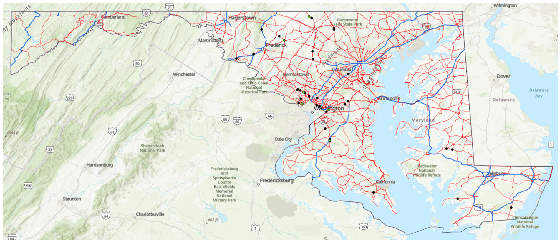
Maryland network and all speed survey spots on the Maryland map.

Methodology

The methodology framework is shown in Figure 2. Data are collected from multiple sources, including speed study reports, probe vehicle data, road geometry, and traffic volumes. Key variables include V₈₅ speeds, segment length, lane width, curb presence, signal and driveway density, PSL, and traffic factors such as AADT, D-factor, and K-factor.

Figure 2.

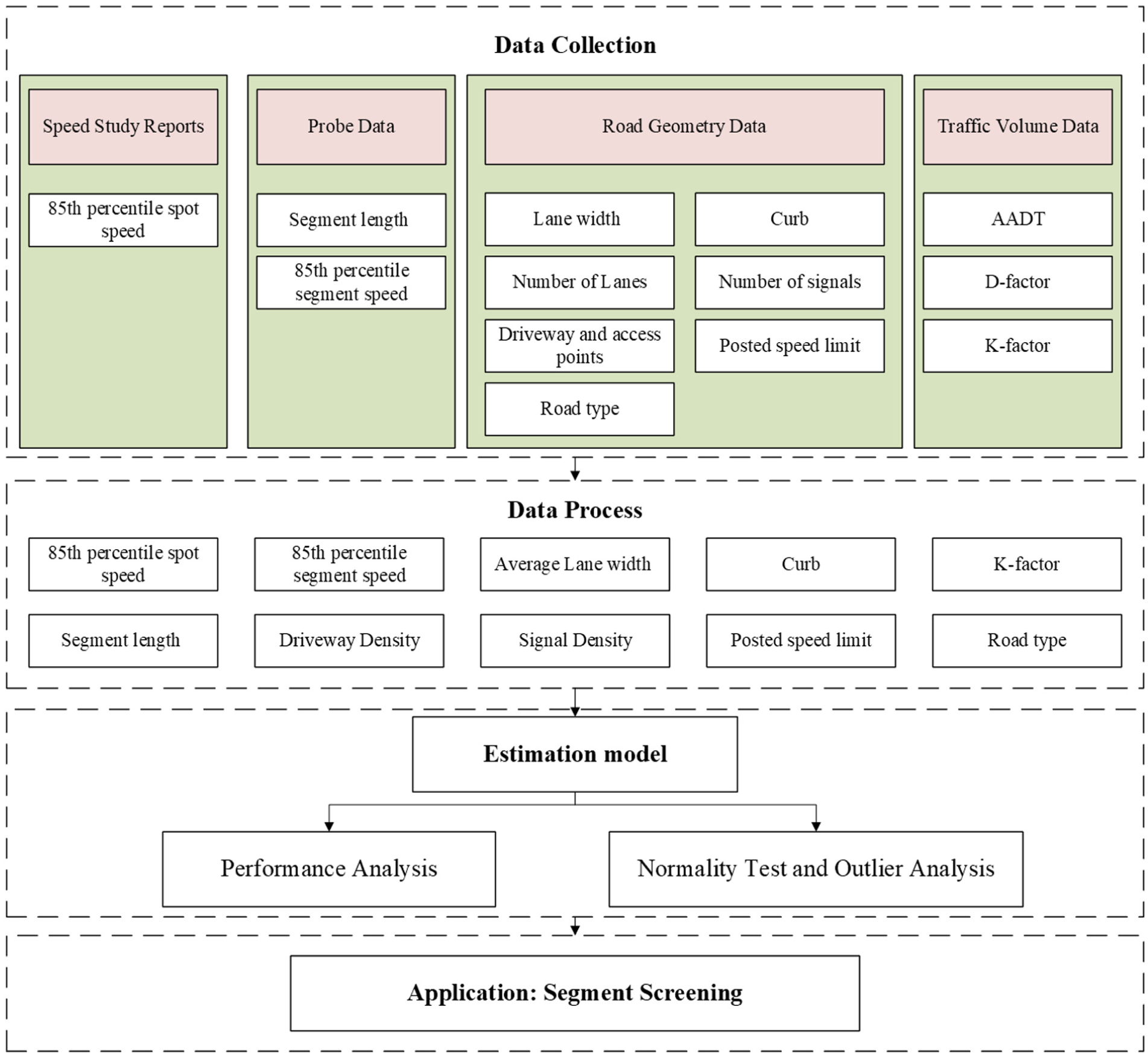
Overview of the research methodology.

After data processing, the selected variables are used to build a regression-based estimation model that predicts V₈₅ spot speeds. The model is evaluated through performance analysis and statistical tests, including normality tests and outlier analysis, to ensure reliability and identify segments where the model performs poorly.

The final model is applied for segment screening by comparing estimated speeds with PSLs. This helps identify road segments that may require attention for speed management or safety review, supporting data-driven decision-making in transportation planning and operations.

The proposed framework clarifies the model structure by specifying the variable combinations, functional forms, and separate regression equations for urban and rural arterials. It provides selected parameter estimates from the literature, but also highlights the need to adjust these coefficients through local calibration when possible, so that local driving behavior and roadway conditions are reflected. These components together make the framework transferable but flexible, supporting practitioners who rely on probe data and limited spot-speed surveys for estimating operating speeds across diverse arterial conditions.

Data Collection and Process

This study aims to develop a forecasting model for percentile speeds. To this end, four datasets were utilized: (1) Maryland speed study reports, (2) probe data, (3) road geometry data, and (4) traffic volume.

Maryland Speed Study Reports

Ground-truth spot V₈₅ values were obtained from Maryland Department of Transportation speed-study reports. Sixty survey sites distributed across both freeways and non-freeway corridors were sampled during campaigns carried out between 2019 and 2025, providing location-specific observations of V₈₅ values, and speed limit against which model estimates can be compared.

Probe Data

Probe-based explanatory variables, sourced from the INRIX Probe Data Analytics, include average speed, reference speed, segment length, functional class, and timestamps for each road segment across the state. Although continuous observations are available from January 1, 2019, to April 1, 2025, only data corresponding to the year of each speed study were extracted for analysis. One-minute records were aggregated into hourly intervals to align with the spot speed-survey data.

Road Geometry Data

Road geometry can also influence percentile speeds. If a road segment has numerous traffic signals or other interruptions, it will affect the space speed, resulting in significantly lower values compared with the percentile spot speed. In this study, road geometry data, including lane width, the number of curbs, signal density, and driveway density, were collected from Google Maps for the corresponding time periods.

Traffic Volume Data

Traffic volume data were obtained from publicly available state-level AADT databases, organized by functional classification. The dataset includes the K-factor, the proportion of daily traffic occurring during the peak hour, and the D-factor, which indicates the directional distribution of peak-hour traffic. Additionally, the number of lanes was recorded for each segment.

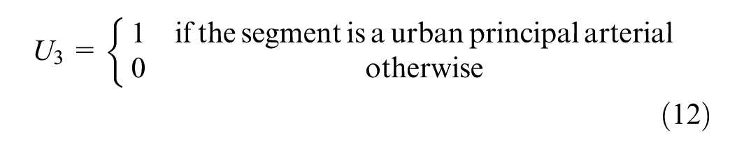
In this section, influential factors associated with the percentile speed estimation are extracted from existing datasets.

1. 85th INRIX segment speed, V_85,seg: The variable V_85,seg denotes the V₈₅ of non-zero speeds for the segment in the INRIX dataset corresponding to the location of the speed survey observation. This value is computed based on hourly average speeds aggregated from records spanning the entire survey year.

2. Segment length, L_seg: The variable L_seg denotes the segment length in the INRIX dataset, measured in miles.

3. Directional AADT per lane, AADT_Lane,Dir: The variable AADT_Lane,Dir denotes the average traffic volume per lane in each direction, thereby capturing directional imbalances in traffic volume for the segment. D-factor, commonly referred to as the directional distribution factor, denotes the proportion of traffic volume traveling in the predominant direction during a specific analysis period, usually the design hour. A higher D-factor implies a significant disparity in traffic volumes between the two directions, suggesting that one direction accommodates the majority of the demand, whereas a 50% D-factor indicates relatively balanced traffic flows. N_Lane,Dir represents the number of lanes in one direction.

\begin{matrix} {AADT}_{Lane, Dir} = \frac{D - factor \times AADT}{N_{Lane, Dir}} \end{matrix}

(1)

4. Average lane width, W_Lane: The W_Lane factor is the average width of each lane in the speed-survey observation spot. W_Dir is the total lane width of the observation direction, measured in feet.

\begin{matrix} W_{Lane} = \frac{W_{Dir}}{N_{Lane, Dir}} \end{matrix}

(2)

5. Curb, C: The curb factor C is a dummy variable to consider the influence of the roadside curb on the percentile speed.

\begin{matrix} C = {\begin{matrix} 1 if the segment has curb \\ 0 otherwise \end{matrix} \end{matrix}

(3)

6. K-factor, K: The variable K is the dimensionless measure that represents the proportion of AADT occurring during the design hour. A higher K indicates that a larger percentage of daily traffic is concentrated within a peak hour, reflecting more pronounced temporal variations in traffic demand. Conversely, a lower K suggests traffic demand is relatively evenly distributed throughout the day.

7. Signal density, $D_{Sig}$ : The variable $D_{Sig}$ represents the number of traffic signals per mile on the segment. $N_{Sig}$ is the total number of signals on the segment.

\begin{matrix} D_{Sig} = \frac{N_{Sig}}{L_{Seg}} \end{matrix}

(4)

8. Driveway density, D_drive: The variable D_drive represents the number of driveways and unsignalized intersections per mile in both directions along the corridor. This variable captures the impact of traffic interruptions caused by driveway access points and unsignalized intersections on corridor speeds. Driveways should be those functioning as traffic generators, such as entrances to schools, retail strips, hospitals, or churches, as they influence the V₈₅. In contrast, driveways serving individual single-family residences, which typically generate minimal traffic, may be assigned a lower weighting per access point, based on engineering judgment.

\begin{matrix} D_{Drive} = \frac{\sum_{dir} w_{1} n_{1} + w_{2} n_{2}}{L_{Seg}} \end{matrix}

(5)

where $w_{1}$ is the weight for the high-impact access points (set as 1); $w_{2}$ is the weight for the low-impact access points (set as 0.5). $n_{1}$ and $n_{2}$ represent the number of high-impact and low-impact access points, respectively.

9. Speed limit, V_p: The variable V_p denotes the PSL at the location of the speed survey at the time the survey was conducted.

10. Speed difference, ΔV: The variable ΔV denotes the difference between V _85,seg and V _p .

\begin{matrix} Δ V = V_{85, Seg} - V_{p} \end{matrix}

(6)

11. Road type: For the rural roads, dummy variables are used to categorize the road type, including rural principal arterial, rural minor arterial, rural major collector, rural minor collector, and rural local roads.

\begin{matrix} R_{3} = {\begin{matrix} 1 if the segment is a rual principal arterial \\ 0 otherwise \end{matrix} \end{matrix}

(7)

\begin{matrix} R_{4} = {\begin{matrix} 1 if the segment is a rual minor arterial \\ 0 otherwise \end{matrix} \end{matrix}

(8)

\begin{matrix} R_{5} = {\begin{matrix} 1 if the segment is a rual major collector \\ 0 otherwise \end{matrix} \end{matrix}

(9)

\begin{matrix} R_{6} = {\begin{matrix} 1 if the segment is a rual minor collector \\ 0 otherwise \end{matrix} \end{matrix}

(10)

\begin{matrix} R_{7} = {\begin{matrix} 1 if the segment is a rual local road \\ 0 otherwise \end{matrix} \end{matrix}

(11)

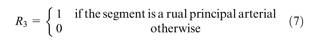
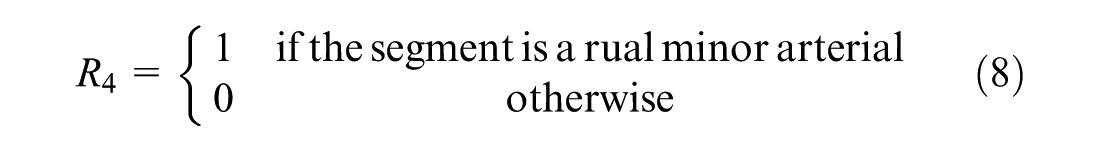
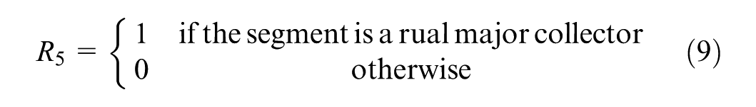
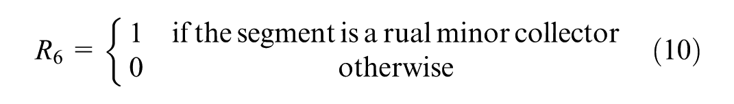
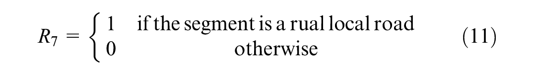
For urban roads, the road types are categorized in urban principal arterial, urban minor arterial, urban major collector, urban minor collector, and urban local roads.

\begin{matrix} U_{3} = {\begin{matrix} 1 if the segment is a urban principal arterial \\ 0 otherwise \end{matrix} \end{matrix}

(12)

\begin{matrix} U_{4} = {\begin{matrix} 1 if the segment is a urban minor arterial \\ 0 otherwise \end{matrix} \end{matrix}

(13)

\begin{matrix} U_{5} = {\begin{matrix} 1 if the segment is a urban major collector \\ 0 otherwise \end{matrix} \end{matrix}

(14)

\begin{matrix} U_{6} = {\begin{matrix} 1 if the segment is a urban minor collector \\ 0 otherwise \end{matrix} \end{matrix}

(15)

\begin{matrix} U_{7} = {\begin{matrix} 1 if the segment is a urban local road \\ 0 otherwise \end{matrix} \end{matrix}

(16)

Regression Model

To estimate the V₈₅ on roadway segments, we employed an OLS regression model. The dependent variable is the observed spot V₈₅ from field surveys, and the independent variables include traffic volume, roadway geometry, and functional classification attributes derived from INRIX segment data and other sources.

The general model is written as:

\begin{matrix} Y = β_{0} + \sum β_{i} X_{i} \end{matrix}

(17)

With the Maryland data listed in the previous section, the V₈₅ model for rural and urban non-freeway segments is proposed using two Maryland spot-speed datasets. The rural dataset comprises surveys from eighteen two-lane and multilane rural highway segments, including minor arterials and major collectors. The urban dataset comprises surveys from forty-two urban highway segments, including two-lane and multilane principal arterials, minor arterials, and major and minor collectors. Each survey site corresponds to a homogeneous roadway segment where geometry, traffic control, and roadside conditions remain approximately constant within the influence area of the speed-measurement station. At each site, field observations were used to obtain the spot 85th-percentile speed, which served as the dependent variable for model development.

Rural Maryland Model

The initial model specification included all available variables that were theoretically relevant and consistently observed across the rural sites in the previous section. To assess multicollinearity, we first examined the Pearson correlation matrix (Figure 3) among continuous variables (excluding dummy indicators) and then computed variance inflation factors (VIFs) for all predictors, retaining K−1 dummies for each categorical variable to avoid the dummy-variable trap ( 17 ). Following common practice, VIF values above ten were treated as evidence of severe multicollinearity

Figure 3.

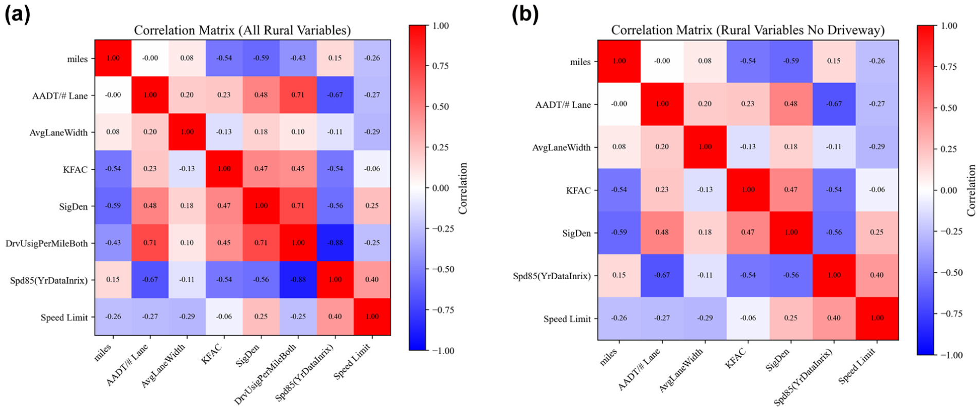
Correlation matrix for rural Maryland model. (a) Correlation matrix with all rural variables and (b) Correlation matrix without driveway.

In the rural dataset, driveway density D _drive exhibited very high correlations with both signal density D _Sig and directional AADT per lane AADT_Lane,Dir, and its VIF exceeded ten. This collinearity arises because, in rural arterial contexts, higher traffic volumes often attract roadside development, leading to a simultaneous increase in both signalized intersections and access points. Therefore, D _drive was removed from the final specification, whereas D _Sig and AADT_Lane,Dir were retained as more interpretable proxies that effectively captured the friction caused by roadside activities. After removing driveway density, all remaining predictors had VIFs below ten (most below five), indicating acceptable levels of multicollinearity for an empirical prediction model (Table 1).

Table 1.

Variance Inflation Factors Rural Maryland Model

Variables	All	Without D_drive
D _drive	18.17026	NA
V _85,seg	16.41424	4.960691
D _Sig	6.351141	6.339601
L _seg	6.198712	2.576058
K	5.566821	4.921849
R ₅	5.339178	4.973758
V _p	3.695438	3.695421
AADT_Lane,Dir	3.684622	3.292228
W _Lane	1.606061	1.568514

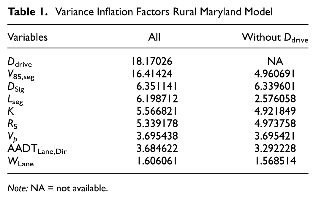
Note: NA = not available.

In summary, based on Pearson correlation and VIF analysis for the rural Maryland model, the final rural model retained segment length L _seg , 85th INRIX segment speed V _85,seg , signal density D _Sig , K-factor K , speed limit V _p , directional AADT per lane AADT_Lane,Dir, and average lane width W _Lane .

Urban Maryland Model

The initial urban model specification included all variables that were theoretically relevant and consistently observed across the urban sites. As in the rural case, we first examined the Pearson correlation matrix (Figure 4) among continuous variables excluding dummy indicators and then computed VIFs for all predictors, retaining K−1 dummies for each categorical variable to avoid the dummy variable trap. VIF values above ten were treated as indicative of severe multicollinearity.

Figure 4.

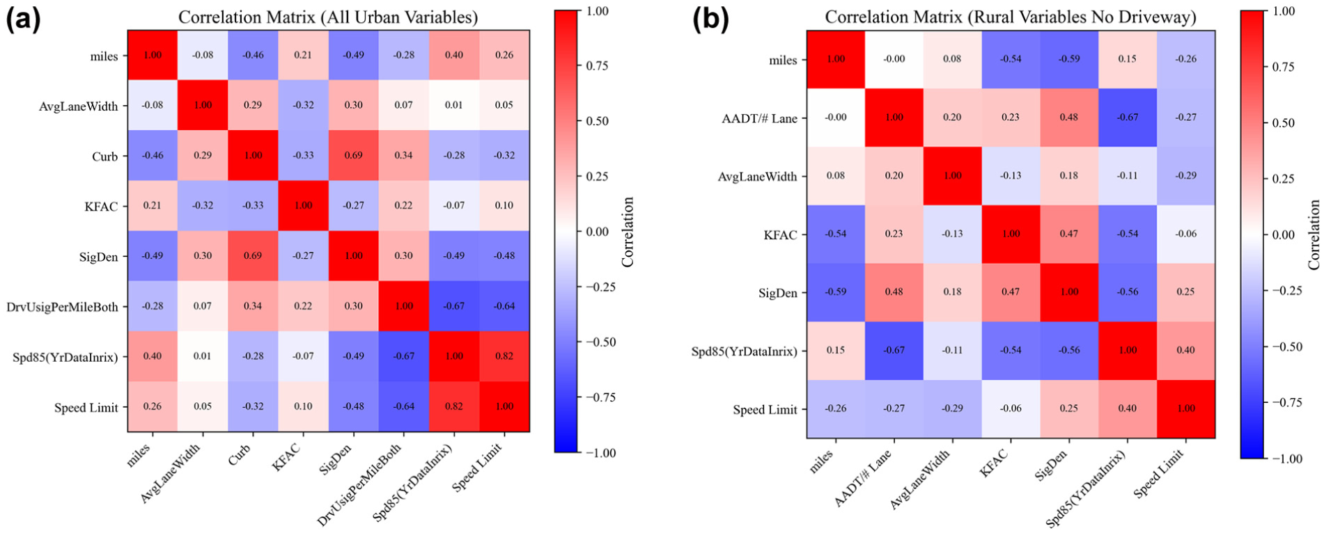
Correlation matrix for urban Maryland model. (a) Correlation matrix with all urban variables and (b) Correlation matrix w/speed difference.

In the initial urban specification, directional AADT per lane AADT_Lane,Dir exhibited a negligible and statistically insignificant effect on spot 85th-percentile speed once geometric design, functional class, and speed variables were controlled for, and its exclusion did not degrade model fit, so it was dropped for parsimony. In addition, 85th INRIX segment speed V _85,seg and speed limit V _p showed a strong pairwise correlation (r ≈ 0.82) and VIFs around 5–6 in the original parameterization. To mitigate this high correlation and improve interpretability, we modified the model by replacing V _p with the difference ΔV (Equation 6), which measures how much the prevailing operating speed exceeds the posted limit. The final urban model therefore includes V _85,seg and ΔV instead of V _p . This reparameterization leaves overall model fit essentially unchanged but reduces the extreme pairwise correlation between the two speed-related predictors to 0.43 and yields moderate VIF values (all below ten, most below five) for the remaining variables, indicating acceptable multicollinearity for an empirical prediction model (Table 2).

Table 2.

Variance Inflation Factors Urban Maryland Model

Variables	All	With ΔV
V _p	5.529485	NA
V _85,seg	4.787778	6.11776418
C	4.145768	4.145767958
D _Sig	3.689745	3.689745488
U ₄	3.602702	3.60270191
D _drive	3.305643	3.305643159
W _Lane	2.278576	2.278575524
U ₅	1.938597	1.938597471
L _seg	1.935156	1.935155618
K	1.92498	1.924980174
ΔV	—	2.251769362

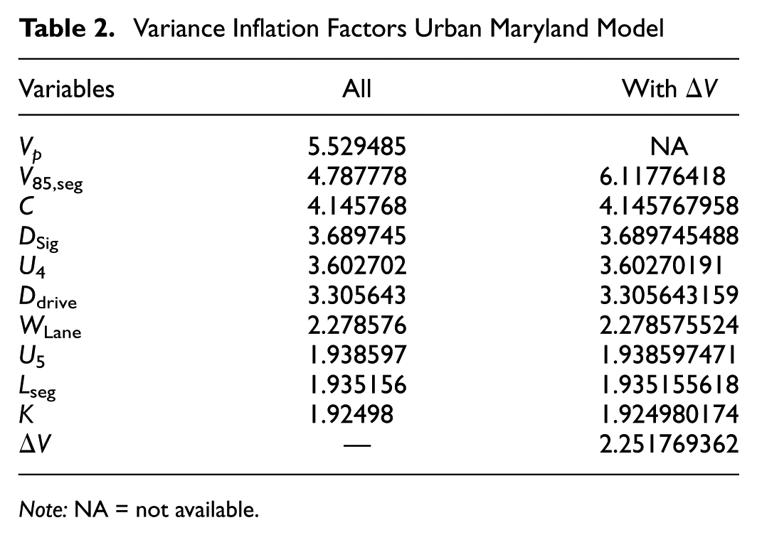
Note: NA = not available.

In summary, based on the Pearson correlation and VIF analysis for the urban Maryland model, the final urban specification retains segment length L _seg , 85th INRIX segment speed V _85,seg , signal density D _Sig , K-factor K , speed difference ΔV, average lane width W _Lane , and driveway density D _drive .

Results

In this section, the model’s performance is first evaluated by comparing it with the estimation model proposed by TTI and a TTI model calibrated using Maryland data. Next, a normality test and outlier analysis are conducted to identify scenarios in which the model performs less effectively. Finally, a case study demonstrates how the model can be applied in practice, using an example to screen other segments.

Performance Analysis

To evaluate the performance of the speed estimation model proposed in this study, we compare it against the percentile speed estimation model developed by TTI, including both the original TTI model and a recalibrated version fitted with Maryland-specific data. The original TTI model (TTI) serves as the baseline, applying parameter estimates derived from the original study. The calibrated Maryland model (Cali_TTI) is a modified version of the TTI model, refitted using Maryland-specific data while excluding speed limit as an explanatory variable.

Table 3 summarizes the estimated coefficients for three model specifications. Each specification is estimated separately for urban (N = 42) and rural (N = 18) arterial segments.

Table 3.

Estimated Coefficients and Confidence Levels by Area Type for V₈₅ Models

	Urban			Rural
Variable	Maryland	TTI	Cali_TTI	Maryland	TTI	Cali_TTI
Constant	1.9594**	27.7463***	0.5407**	40.4202	9.6910***	68.3548
L _seg	0.4397	−0.575	−2.6977	−5.5875	−0.4915**	15.6614
AADT_Lane,Dir	NA	0.00027***	−0.00005	−0.0002	0.0001***	0.0001
W _Lane	2.8377***	−0.2743***	3.3657***	−0.8166	−0.3492***	−6.2941
C	0.6842	NA	−0.0330	NA	−0.6686***	NA
K	−1.8057***	−0.3821***	−1.1568	−0.1580	−0.0762***	−3.3219
U ₃ or R₃	−6.7922**	−0.1088	0.0240	NA	1.4641***	NA
U ₄ or R₄	−5.3732*	2.1511***	−0.5686	22.4771*	1.1702***	32.6777
U ₅ or R₅	−6.5502**	1.2176***	−2.0380	17.9431	−0.5285*	35.6771
U ₆ or R₆	NA	NA	NA	NA	−0.8189	NA
U ₇ or R₇	NA	−3.2599	2.1230	NA	−1.2869	NA
D _Sig	0.0338	−0.4612***	−0.4830	−5.5232**	−2.4241***	2.2031
D _Drive	−0.4033	−0.0095***	−0.7342**	NA	−0.1920***	0.6706
V _85,seg	0.8483***	0.7738***	0.6150***	−0.6855*	1.0213***	0.8134
V _p	NA	NA	NA	0.9628***	NA	NA
ΔV	−0.3991**	NA	NA	NA	NA	NA

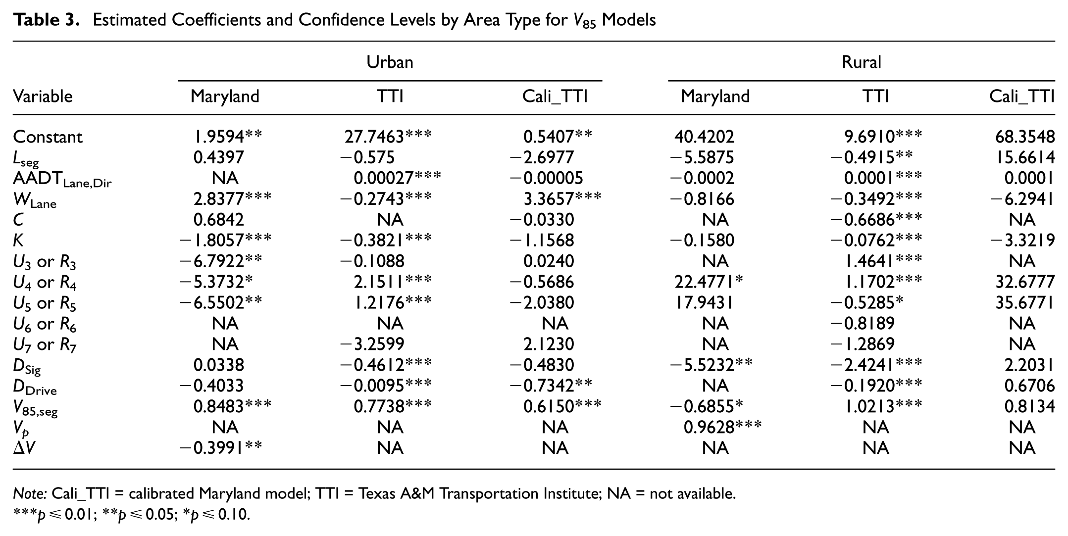
Note: Cali_TTI = calibrated Maryland model; TTI = Texas A&M Transportation Institute; NA = not available.

***p ≤ 0.01; **p ≤ 0.05; *p ≤ 0.10.

From Table 4, in urban areas, all models achieve relatively high R² values, indicating good explanatory power. Although the TTI model achieves a higher R² than the Maryland model, its mean absolute percentage error (MAPE) is much larger; therefore, despite tracking the overall speed pattern well, the TTI model systematically over- or underestimates, leading to greater prediction error. In rural areas, the Cali_TTI model performed poorly, as excluding the speed limit did not capture actual operating speeds. The strong correlation (0.71) between PSL and actual V₈₅ indicates that the speed limit is the most important predictor. This is confirmed by the model results: excluding PSL reduced the R² to 0.014, whereas including it improved the R² to 0.751. Note that unlike the TTI context where geometric variables or stronger INRIX data effectively captured operating speeds, the lower INRIX correlation (0.42) in Maryland necessitates PSL as a calibration tool. This indicates that probe data remain valuable but require PSL as a correction factor for reliable rural estimation.

Table 4.

R ² and Mean Absolute Percentage Error (MAPE) of Urban and Rural V₈₅ Estimation Models

Model	R ²	MAPE (%)
Urban
TTI	0.881	18.7
Maryland model	0.841	4.7
Cali_TTI	0.808	5.0
Rural
TTI	0.727	7.9
Maryland model	0.751	2.5
Cali_TTI	0.014	4.4

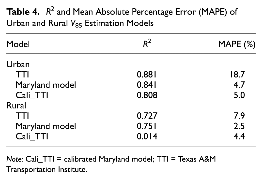
Note: Cali_TTI = calibrated Maryland model; TTI = Texas A&M Transportation Institute.

With regard to prediction error, the Maryland model clearly outperforms the alternatives in both settings. In urban segments, the Maryland model yields the smallest MAPE (4.7%), with the Cali_TTI model slightly higher (5.0%) and the original TTI model much less accurate (18.7%). In rural segments, the Maryland model again produces the lowest MAPE (2.5%), compared with 7.9% for the TTI model and 4.4% for the Cali_TTI model. It is worth noting that although the rural Cali_TTI model shows a low MAPE (4.4%), this should be interpreted with caution. Its negligible R² suggests the model fails to explain the variance in operating speeds, implying that the low error rate is merely an artifact of the data distribution rather than a sign of predictive reliability. Thus, when PSL is omitted, prediction errors increase in both rural and urban applications, and the rural Maryland case in particular shows that a model calibrated with PSL provides substantially more reliable estimates of spot 85th-percentile speed.

Taken together, these results suggest that the posted speed limit is an important predictor in both urban and rural contexts, especially when only a small number of local calibration sites are available. In urban segments, congestion, signal density, and geometric design undoubtedly shape operating speeds, yet the Maryland model that includes PSL still achieves the lowest MAPE. This indicates that even where traffic control and geometry play a dominant role, PSL provides additional explanatory power and helps stabilize the model under limited-sample conditions. In rural segments, the effect of PSL is even more pronounced: omitting it leads to substantially larger prediction errors, whereas the Maryland model with PSL captures observed V₈₅ much more accurately. This pattern is consistent with the idea that rural PSLs tend to align closely with prevailing driver behavior under relatively simple and unconstrained operating conditions.

In addition, the statistical relationship we observe between PSL and V₈₅ reflects the type of connection addressed in the MUTCD guidance, which states: “On a freeway, expressway, or rural highway (outside urbanized locations or conditions), the speed limit that is posted within a speed zone should be within 5 mph of the 85th-percentile speed of free-flowing motor-vehicle traffic under the following conditions.” This reflects a widely adopted practice in which PSLs are often adjusted based on measured operating speeds. Although our model does not determine a causal direction between PSL and V₈₅, it reveals a strong statistical relationship. As V₈₅ increases, there may be upward pressure to raise PSL; similarly, higher PSL segments tend to show higher V₈₅. This bidirectional relationship suggests that speed limits not only influence driver behavior but may also reflect it.

In brief, rather than being excluded in the previous model, PSL serves as a useful variable in both urban and rural Maryland. Incorporating PSL improves predictive reliability and helps bridge the gap between probe-based speed indicators and field-measured spot speeds. This finding aligns with the literature ( 8 ): in urban areas, PSL is strongly shaped by geometric and operational constraints but still carries residual information about drivers’ speed choices, whereas in rural areas, where alignment and control are simpler, PSL can reasonably be treated as an independent term that directly captures the intended operating regime.

Normality Test and Outlier Analysis

To evaluate the suitability of the regression model and verify that key assumptions hold, a normality assessment was conducted on the prediction errors. Figure 5 shows that the residuals are approximately normally distributed, with a symmetric, bell-shaped pattern centered around zero and no evident skewness or extreme outliers. This visual observation is supported by the results of three established normality tests. The Shapiro–Wilk test yields a test statistic of 0.981 and a p-value of 0.360, indicating that the null hypothesis of normality cannot be rejected. The D’Agostino–Pearson omnibus test produced a p-value of 0.204, further supporting the assumption of normality. The Anderson–Darling test returned a test statistic of 0.486, which is below all critical values (minimum = 0.548), confirming the absence of significant deviation from a normal distribution.

Figure 5.

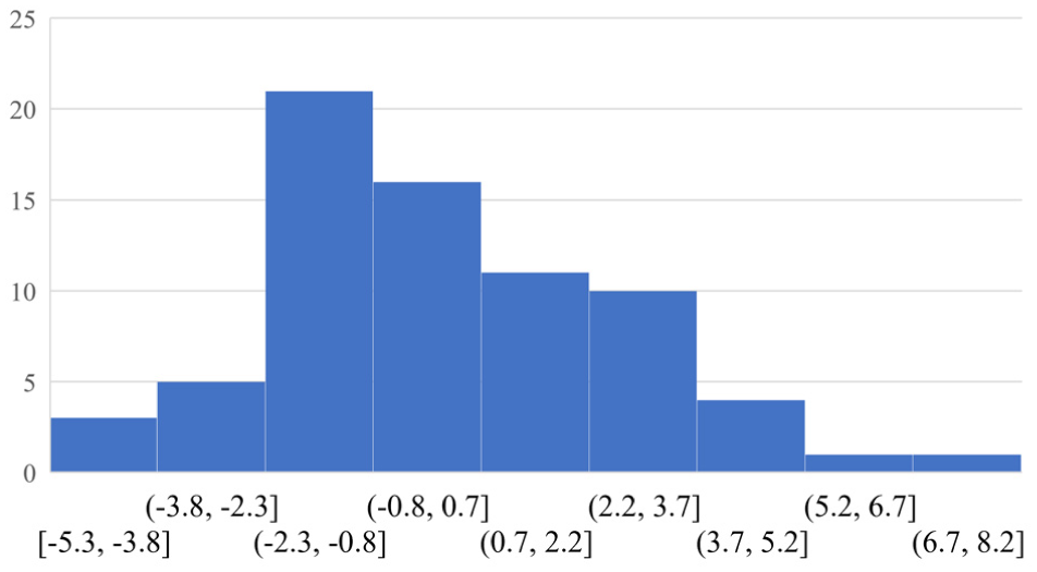
Prediction error distribution.

In addition to the normality check, an outlier analysis was conducted to identify conditions where the model may underperform and to understand sources of large prediction errors. Using the standard deviation of prediction errors σ of 2.51 mph and a mean residual of 0.20 mph, a 95% confidence interval was defined as [−4.72, 5.11] mph. Prediction errors lying outside this range were flagged as outliers for further investigation.

Six segments illustrating a range of deviations between predicted and actual V₈₅ values were selected to examine contexts associated with both high and minimal prediction errors (Table 5):

Table 5.

Comparison of Prediction Accuracy Across Selected Segments

Segment	V _p	Actual V₈₅	Predicted V₈₅	Road type	D _Sig	Access points	Performance assessment
MD 14 at Cloverdale	50	56	55.6	R5	0	6	Good fit
US 1 North of Dr Patel Drive	45	48	47.6	U3	1	10	Good fit
MD 12 at Coolspring United Methodist Church	50	60	57.4	R5	0	6	Underestimated
MD 586 at Bushey Drive	40	48	43.5	U3	4	8	Underestimated
MD 363 in Dames Quarter	40	44	46.4	R5	0	5	Overestimated
MD 450 at Cornerstone Church Drive	45	40	47.9	U5	2	7	Overestimated

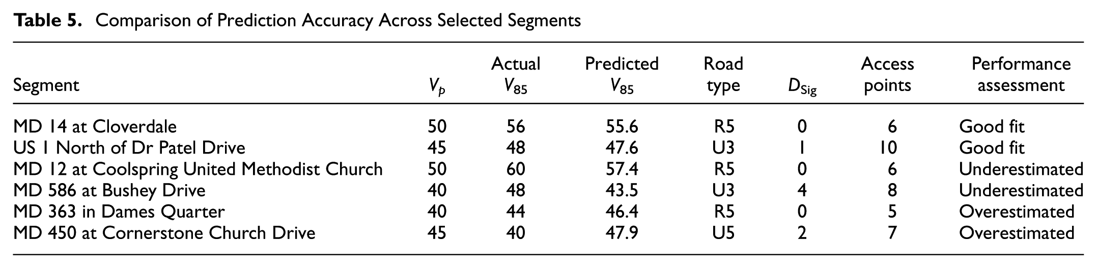
Segments with minimal prediction errors, such as MD 14 at Cloverdale and US 1 (north of Dr. Patel Drive), represent typical arterial environments where the model effectively captures V₈₅. The rural segment (MD 14) features linear geometry with negligible roadside interference, resulting in a predictable driving environment where behavior is heavily dependent on V_p and roadway class. Similarly, the urban segment (US 1) exhibits the characteristics of a straight suburban arterial. Despite the presence of commercial access points and townhouse entrances, the segment maintains near free-flow conditions, as the disturbances from access points are insufficient to significantly disrupt traffic momentum. In both instances, the absence of unexpected geometric constraints ensures that V_p serves as the primary determinant, allowing the model to accurately estimate V₈₅.

The model underestimates V₈₅ at MD 12 at Coolspring United Methodist Church and MD 586 at Bushey Drive, with prediction gaps of 2.6 mph and 4.5 mph, respectively. For the rural segment (MD 12), the underestimation is likely driven by a directional disparity in V_p. With opposing traffic streams subject to different regulatory limits (30 mph versus 40 mph), the environment lacks uniformity, potentially prompting drivers to disregard the lower limit in favor of a higher V₈₅ consistent with the faster direction. Meanwhile, the urban segment (MD 586) represents a high-density residential corridor with frequent signalized intersections (D_Sig = 4). This suggests that the model tends to underestimate speeds in sections with aggressive driving behavior. Although geometric variables such as D_Sig imply lower speeds, actual driving patterns in this corridor consistently exceed the speed reductions expected from the signal density, resulting in observed speeds that are higher than model predictions.

Conversely, the model overestimated speeds for MD 363 in Dames Quarter. This rural major collector segment represents a transition zone, with the PSL decreasing from 50 mph to 40 mph. It appears the model does not fully account for the influence of transitional speed limits, which often cause drivers to slow down in anticipation of the upcoming lower limit. Similarly, an overestimation occurred along MD 450 at the Cornerstone Church Drive segment. Although the segment is designated as an urban major principal arterial, the actual V₈₅ was lower than the estimated speed. For this segment, the PSL increases from 30 mph to 45 mph along the eastbound direction, so drivers may have accelerated in anticipation of the higher limit ahead, resulting in an observed V₈₅ that is higher than the model would expect for the current zone.

Overall, this analysis illustrates that the accuracy of V₈₅ prediction is not solely dependent on physical roadway attributes but is also influenced by nuanced driver behavior and context-specific factors. These findings suggest that careful calibration and clearer subclassification of variables (e.g., differentiating high- and low-impact driveways) are needed when generalized models are applied to specific sites.

Case Study: Application of the Model for Segment Screening

This case study demonstrates the utility of the proposed model as a planning and screening tool for identifying road segments with substantial discrepancies between PSLs and predicted V₈₅ (Figure 6). The model can be useful in contexts where spot speed studies are not available, supporting data-driven decisions such as setting or modifying speed limits, calibrating crash-prediction models, and determining eligibility conditions for traffic safety countermeasures.

Figure 6.

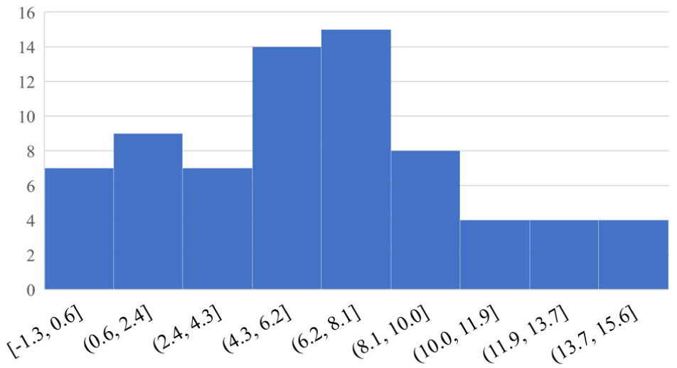
Difference between speed limits and estimated V₈₅.

For demonstration purposes, the study defines extreme cases as those where the predicted V₈₅ exceeds the PSL by more than 12 mph, or where the predicted V₈₅ falls below the speed limit. A total of two cases are identified below:

MD 97 @ Old Hanover Rd (V₈₅ is 15.6 mph Higher than the Speed Limit)

This segment lies within a rural speed transition zone where the posted speed limit drops from 45 mph to 35 mph. Drivers approaching from the upstream 45 mph section tend to maintain their higher speed as they enter the lower-speed zone, so most vehicles substantially exceed the 35 mph limit. The site is located on a two-lane, two-way rural highway with noticeable rolling grades, and the combination of downhill approaches and limited vertical sight distance likely contributes to the observed high operating speeds. A high V₈₅ in this context may pose a safety concern for both through traffic and turning vehicles. Potential countermeasures include extending the speed reduction over a longer distance, enhancing advance warning and speed limit signage, and considering automated speed enforcement.

MD 30BU @ Trenton Mill Rd (V₈₅ is 1.3 mph Lower than the Speed Limit)

This segment is located on an urban arterial where the upstream section is posted at 30 mph and includes a signalized railroad crossing. Drivers approaching from the upstream side tend to be cautious because of the rail crossing and associated traffic control, often decelerating in advance and proceeding carefully through the intersection. As a result, when vehicles enter the downstream segment, which is posted at 50 mph, their speeds may still be recovering from the upstream control and have not yet increased to match the higher posted speed limit. In this case, the observed V₈₅ being slightly below the 50 mph PSL does not immediately indicate a safety concern; rather, it reflects prudent driver behavior in response to upstream constraints. Nonetheless, it may suggest an opportunity to review the coordination of signals, signing, and speed zoning along the corridor to ensure that speed expectations are clear and that operating speeds transition smoothly between adjacent segments.

Conclusions

This study developed a Maryland-calibrated regression model for estimating 85th-percentile speed (V₈₅) on non-freeway arterials and benchmarked it against both the original and locally calibrated TTI models. By incorporating PSL and a directional AADT term, the proposed model lowered the mean absolute error to roughly 5 mph, about 60% below the uncalibrated TTI model and 25% below the Maryland-tuned model, while relying on only 60 spot-speed surveys. Outlier diagnostics further revealed that the largest residuals arise in speed-transition zones, segments with sparse driveway counts but active roadside development, and sites affected by probe-data dropouts.

This study validates that direct model transfer is not always feasible and helps clarify the ambiguity about the role of the PSL in operating-speed models. Although geometric features effectively substituted for PSL in the original Texas context, they failed to replicate such predictive power in rural Maryland. These results indicate that true transferability requires context-aware local calibration: treating PSL as an essential predictor in rural environments.

The findings have practical implications for transportation agencies. First, transportation agencies can deploy the model as a cost-effective surveillance tool, using readily available probe data and roadway attributes to prioritize locations for detailed study. Second, the quantified influence of PSL provides a transparent criterion for deciding when its inclusion is essential, for example, on homogeneous rural corridors, and when a leaner specification may suffice in dense urban non-freeways. Third, the model’s diagnostic capability directs practitioners toward specific countermeasures such as improved transition-zone signing, driveway-access management, or enforcement in lanes with marked directional imbalance.

Some limitations exist in this study. The analysis is confined to non-freeway arterials because concurrent probe-speed and spot-survey data were unavailable for limited-access facilities; extending the approach to freeways remains a priority. Although rigorous filtering was applied, residual noise and gaps in the probe dataset could bias coefficient estimates. Another limitation of the model is that it treats all access points equally, potentially biasing estimates by not distinguishing between high- and low-impact driveways, though future work could explore weighted or land-use-based classifications to improve accuracy.

Future work should therefore pursue the following directions. First, additional spot-speed data on freeways would permit testing the model’s applicability across the full roadway hierarchy. Second, systematic experiments are needed to formalize when PSL improves prediction accuracy and when it can be safely omitted, balancing parsimony and performance. Third, integrating land-use may refine driveway and access metrics, potentially eliminating the rural outliers identified here. Fourth, as larger datasets become available, exploring hybrid approaches that pair interpretable regression with non-linear methods (e.g., machine-learning residual correctors) could further improve prediction accuracy while maintaining transparency. Finally, as comparable spot-speed and probe datasets from other states become available, the proposed framework could be evaluated through cross-jurisdictional validation (e.g., training on Maryland and testing on another state, and vice versa) to assess which components are transferable and which require region-specific recalibration.

Footnotes

Authors’ Note

The authors acknowledge that a large language model, ChatGPT, was used and only used in improving the language when preparing the manuscript. The authors acknowledge the limitations of language models, and the accuracy, validity, and appropriateness of written language have been rigorously verified by the authors. The manuscript was prepared with assistance from the ChatGPT o3 model for code development and manuscript language improvement.

Author Contributions

The authors confirm contributions to the paper as follows: study conception and design: Y. Zhang and Y. Choi; data collection: Y. Zhang and Y. Choi; analysis and interpretation of results: Y. Zhang and Y. Choi; draft manuscript preparation: Y. Zhang, Y. Choi, and X. Yang. All authors reviewed the results and approved the final version of the manuscript.

Declaration of Conflicting Interests

The authors declared the following potential conflicts of interest with respect to the research, authorship, and/or publication of this article: Xianfeng (Terry) Yang is a member of Transportation Research Record’s Editorial Board. All other authors declared no potential conflicts of interest with respect to the research, authorship, and/or publication of this article.

Funding

The authors received no financial support for the research, authorship, and/or publication of this article.

ORCID iDs

Yi Zhang

Xianfeng (Terry) Yang

Data Accessibility Statement

The data that support the findings of this study are available from the corresponding author on reasonable request, subject to applicable restrictions.

References

Forbes

Gardner

McGee

R. Srinivasan . Methods and Practices for Setting Speed Limits: An Informational Report. Publication FHWA-SA-12-004. Federal Highway Administration, Washington, D.C., 2012.

Fitzpatrick

Blaschke

J. D.

B. Shamburger

Krammes

R. A.

Fambro

D. B.

Compatibility of Design Speed, Operating Speed, And Posted Speed. Federal Highway Administration, Washington, D.C., 1995.

Federal Highway Administration. Manual on Uniform Traffic Control Devices for Streets and Highways 11th Edition. Washington, D.C., 2023.

American Association of State Highway and Transportation Officials. Highway Safety Manual, 2014 Supplement. Washington, D.C., 2014.

Federal Highway Administration. Traffic Calming EPrimer. Washington, D.C. https://highways.dot.gov/safety/speed-management/traffic-calming-eprimer. Accessed June 9, 2026.

Morrall

J. F.

Talarico

R. J.

Side Friction Demanded and Margins of Safety on Horizontal Curves. Transportation Research Record: Journal of the Transportation Research Board, 1994. 1435: 145–152.

Islam

Seneviratne

Evaluation of Design Consistency of Two-Lane Rural Highways. ITE Journal, Vol. 64, No. 2, 1994, pp. 28–31.

Wang

Dixon

K. K.

Hunter Wang

M. J.

Hunter

Operating-Speed Model for Low-Speed Urban Tangent Streets Based on In-Vehicle Global Positioning System Data. Transportation Research Record: Journal of the Transportation Research Board, 2006. 1961: 24–33.

Himes

S. C.

Donnell

E. T.

Porter

R. J.

Posted Speed Limit: To Include or Not to Include in Operating Speed Models. Transportation Research Part A: Policy and Practice, Vol. 52, 2013, pp. 23–33. https://doi.org/10.1016/j.tra.2013.04.003.

10.

Fitzpatrick

Carlson

Brewer

Wooldridge

Miaou

Design Speed, Operating Speed, and Posted Speed Practices. NCHRP Report 504. Transportation Research Board of the National Academies, Washington, D.C., 2003.

11.

Fitzpatrick

Kutela

Park

E. S.

Pratt

M. P.

Venglar

Using Vehicle Probe Data To Evaluate Speed Limits. Publication FHWA/TX-24/0-7156-R1. Federal Highway Administration, Washington, D.C., 2024.

12.

Lan

Zhao

Selection of an Appropriate Reference Speed for the Calculation of Highway Performance Measures. Publication FHWA/VTRC 25-R21. Federal Highway Administration, Washington, D.C., 2025.

13.

Singh

Zaman

White

Neural Network Modeling of 85th Percentile Speed for Two-Lane Rural Highways. Transportation Research Record: Journal of the Transportation Research Board, 2012. 2301: 17–27. https://doi.org/10.3141/2301-03.

14.

Semeida

A. M.

Application of Artificial Neural Networks for Operating Speed Prediction at Horizontal Curves: A Case Study in Egypt. Journal of Modern Transportation, Vol. 22, No. 1, 2014, pp. 20–29. https://doi.org/10.1007/s40534-014-0033-3.

15.

Guo

Sivakumar

Dong

Krishnan

Transferability Improvement in Short-Term Traffic Prediction Using Stacked LSTM Network. Transportation Research Part C: Emerging Technologies, Vol. 124, 2021, p. 102977. https://doi.org/10.1016/j.trc.2021.102977.

16.

Sikder

Pinjari

A. R.

Srinivasan

Nowrouzian

Spatial Transferability of Travel Forecasting Models: A Review and Synthesis. International Journal of Advances in Engineering Sciences and Applied Mathematics, Vol. 5, 2013, pp. 104–128.

17.

Wooldridge

J. M.

Introductory Econometrics: A Modern Approach. CENGAGE Learning, U.S., 2016.

Estimating Percentile Speeds with Probe Vehicle Data on Non-Freeways

Abstract

Keywords

Introduction

Literature Review

Role of the 85th Percentile Speed

Models for Estimating 85th Percentile Speed

Model Transferability and Local Calibration

Research Area

Methodology

Data Collection and Process

Maryland Speed Study Reports

Probe Data

Road Geometry Data

Traffic Volume Data

Regression Model

Rural Maryland Model

Urban Maryland Model

Results

Performance Analysis

Normality Test and Outlier Analysis

Case Study: Application of the Model for Segment Screening

MD 97 @ Old Hanover Rd (V85 is 15.6 mph Higher than the Speed Limit)

MD 30BU @ Trenton Mill Rd (V85 is 1.3 mph Lower than the Speed Limit)

Conclusions

Footnotes

Authors’ Note

Author Contributions

Declaration of Conflicting Interests

Funding

ORCID iDs

Data Accessibility Statement

References

MD 97 @ Old Hanover Rd (V₈₅ is 15.6 mph Higher than the Speed Limit)

MD 30BU @ Trenton Mill Rd (V₈₅ is 1.3 mph Lower than the Speed Limit)