






Abstract
This paper investigates strategies to enhance the performance of deep learning models in pavement distress detection by utilizing two distinct datasets collected and annotated from different sources (vendors). The datasets consist of two- and three-dimensional images scanned from asphalt/concrete pavements and manually labeled for multiple surface distresses. Despite using the same base model to train individually, the performance of new models varies between the two datasets for the same pavement type. It remains a question whether transfer learning, knowledge distillation, or data merging will improve weaker models by leveraging stronger ones and increase the models’ robustness across different data sources. Experiments are conducted using these strategies to assess their applicability for single-source data (e.g., from a single vendor) and their generalization for multiple sources (e.g., from two or more vendors). This paper bridges a knowledge gap by qualitatively and quantitatively evaluating the effects of these strategies on current pavement distress detection practices using image data. Optimal approaches, such as fine-tuning or data merging, are recommended for various use cases aimed at real applications.
Keywords
Introduction
Road networks are a crucial infrastructure that deteriorates over time because of aging, weathering, and extreme events. Timely monitoring is essential for effective maintenance and repair, which can preserve performance and extend service life. Many US states have already adopted advanced technologies, such as high-resolution cameras and laser sensors, to collect road surface data and assess conditions for maintenance decisions ( 1 ). Among these, line laser imaging systems capture two-dimensional (2D) intensity images (distress looks) and three-dimensional (3D) range images (depth information obtained from the laser triangulation) ( 2 ). High-resolution cameras in these systems can detect distress with a precision of 0.3–1.0 mm ( 3 – 5 ). However, manual inspection by human experts is infeasible on a scale of the vast volume of collected images. Recently, artificial intelligence (AI) and deep learning, particularly convolutional neural networks (CNNs), have demonstrated superior performance in automatic detection of various pavement surface distresses with 2D/3D imagery.
Previous research found that fused 2D/3D images improve detection accuracy, even when paired with generative AI methods, on a prepared dataset ( 6 – 8 ). In this paper, a new challenge is addressed: two vendor datasets with identical distress definitions but different formats. Both data sets include bounding-box-labeled distresses for asphalt concrete pavement (ACP) and continuously reinforced concrete pavement (CRCP). Dataset 7150 has a resolution of 1,536 × 900 pixels covering a pavement surface with a width of 4.3 m and a length from 1.0 to 8.1 m, depending on the driving speed. Dataset NSF, at a resolution of 4,096 × 2,048 pixels, and covers a 4.3 × 14.3-m pavement region. This is achieved because a distance measurement unit triggers the line laser camera at fixed intervals (e.g., 7 mm) for scanning ( 7 ). These two datasets exhibit visual disparities because of optical devices, lighting, and road types (see Figure 1). Models trained on one dataset often perform poorly on the other, even without accuracy on their native data after a new training is applied. This raises the question of how to properly utilize datasets and trained models for robust pavement surface defect detection.
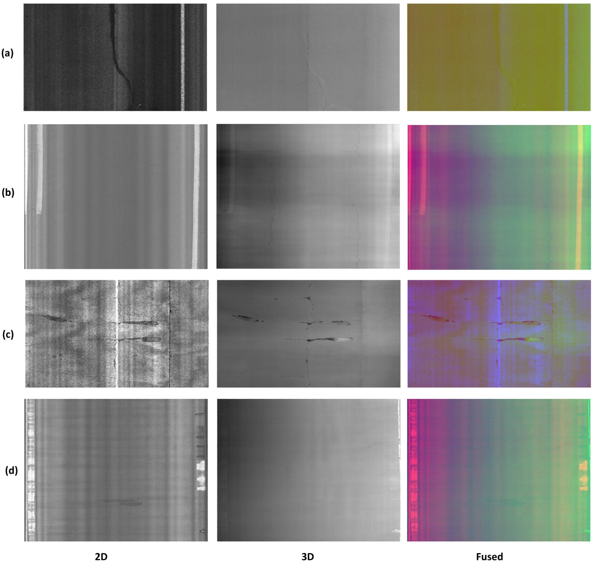
Two datasets collected in this paper (from left to right, these are two-dimensional (2D), three-dimensional (3D), and fused images): (a) and © are examples of ACP and CRCP for Datasets 7150 and NSF; (b) and (d) are examples of ACP and CRCP for Datasets 7150 and NSF.
This paper aims to enhance the accuracy, generalization, and versatility of deep learning models for automated pavement distress detection, particularly when handling new datasets from different vendors or with varying distress definitions using 2D/3D image data. To address the “black-box” nature of deep learning, four strategies are rigorously evaluated: (1) merging datasets; (2) fine-tuning pretrained models; (3) freezing initial layers for knowledge transfer; and (4) knowledge distillation (KD) between fine-tuned models. Utilizing the You Only Look Once version 11 (YOLO) model, this paper addresses a critical knowledge gap in automated pavement distress detection: Given available datasets, what represents the best strategy for effectively leveraging two distinct datasets, independent of deep learning model selection?
Related Work
Pavement distress detection, classification, and segmentation have long been active research areas with vision-based technologies. Early approaches primarily relied on digital image processing techniques, as illustrated in Fukuhara et al. ( 9 ), Mahler et al. ( 10 ), Georgopoulos et al. ( 11 ), and Abbas and Ismael ( 12 ). Recent advances have shifted toward deep learning methods using 2D/3D image data for automated pavement distress identification. This paper focuses on effective utilization of 2D/3D image data and different deep learning architectures, and efficient techniques to extract transferable knowledge that can improve the model’s performance and generalization under diverse pavement conditions.
Pavement Distress Detection Using Deep Learning and 2D or 3D Images
The use of 2D images for automated pavement distress detection has been extensively researched using various vision-based deep learning approaches. Several studies have shown the effectiveness of different methodologies. Du et al. ( 13 ) achieved a 73.64% detection accuracy using YOLOv3 on 45,788 high-resolution images annotated for various distress types, including longitudinal/transverse cracks, alligator cracks, potholes, and manholes. Alternative approaches include the wavelet transform method, which separates distress features from noise using amplitude analysis by Zhou et al. ( 14 ). The Faster R-CNN framework, applied to 3,700 × 10,000 images but cropped to 1,865 × 2,000 for crack detection by Ibragimov et al. ( 15 ), is another example. Recent advances have focused more on improving model architectures and efficiency, such as YOLOv5 with Shuffle Attention and Swin-Transformer trained on 2,460 images with a size of 2,048 × 2,000 in Liu et al. ( 16 ), a lightweight Generative Adversarial Network for small 160 × 160 images ( 17 ), and the lightweight feature-enhanced YOLO for real time detection ( 18 ). Data creation and preprocessing methods vary significantly among studies, from a collection of 50,000 road images using vehicle-mounted cameras ( 19 ) to a 20,000-image dataset (cropped from larger 3,704 × 10,000 scans) labeled with crack severity ( 20 ). Other notable contributions include Mamba-based detection with 13,129 images at 1,024 × 1,024 in Sun et al. ( 21 ), YOLOv7 implementation on 5,898 scans at 2,048 × 2,048 covering various distress types in Dan et al. ( 22 ), and extensive testing on 60,059 high-resolution images in Tang et al. ( 23 ). Recent innovations have introduced novel architectures such as the Transformer Patch Labeling Network by Huang et al. ( 24 ) and hybrid approaches such as an end-to-end pipeline combining YOLOv5 with new metrics in Cano-Ortiz et al. ( 25 ). Inspired by these applications with the YOLO, YOLOv11 is selected as the base model to train two different datasets in this paper.
2D/3D imagery has become an important data source for automated pavement distress detection and segmentation because it enables more comprehensive analysis. Several advanced approaches have been developed to fully use these imaging modalities: Wang ( 4 ) established foundational methods to survey pavement distresses using 2D/3D laser images, while Zhang et al. ( 26 ) later proposed an enhanced ShuttleNet architecture specifically designed for multiclass distress segmentation. In total, 5,763 high-resolution images, processed from an original size of 4,096 × 2,048 covering 4 × 2-m pavement surfaces to a size of 512 × 256, were used to identify cracks, potholes, seal cracks, patches, markings, and expansion joints. Lang et al. ( 3 ) developed the Pavement Distress Segmentation Network (PDSNet), a combination of PSPNet and U-Net architectures. The PDSNet was trained on 12,648 2D/3D images by downsampling from 2,048 × 2,048 to 512 × 512 and maintaining 0.35-mm elevation accuracy to segment diverse distress types, including sealed cracks, patching, potholes, raveling, bridge joints, and pavement markings. Sun and Qian ( 27 ) contributed a multiscale wavelet transform method specifically optimized for crack delineation. These studies collectively indicated the evolution of pavement assessment techniques, from early aerial 2D imaging applications to sophisticated laser-scan 3D imaging and hybrid networks capable of processing 2D and 3D data for distress detection and analysis. This paper is a continuous study of how to mine deep using 2D/3D image datasets with deep learning.
Transfer Learning and KD in Pavement Distress-related Research
Transfer learning (TL) has proven highly effective for pavement distress detection by adapting pretrained models to diverse data conditions. Most previously reviewed papers used TL in the research, but the following research discussed it more specifically. Gopalakrishnan et al. ( 28 ) fine-tuned an ImageNet-trained Visual Geometry Group model for crack detection on various pavement types. Subsequent advances have been made, including a cross-scene pipeline that combines domain adaptation and CycleGAN-based image conversion for multiview datasets (29), and a data fusion and transfer learning with YOLO (YOLO-DFT) framework with cloud-based label fusion ( 30 ). Wen et al. ( 31 ) achieved pixel-level segmentation of 4,000 annotated images for potholes, raveling, patches, and sealed cracks on roads using TL skills. These approaches indicate the ability of TL to address data scarcity, viewpoint variations, and annotation challenges, and how model generalization can be increased in pavement condition monitoring and assessment. TL techniques are the main strategies used in this research.
KD has emerged as a powerful technique for improving the efficiency and accuracy of pavement distress and infrastructure damage detection. Zhang et al. ( 32 ) applied this approach to bridge the gap between patch- and image-based classification, distilling knowledge into an EfficientNet-B3 model and testing it on a large-scale bituminous pavement dataset. Meng et al. ( 33 ) developed a KD model with multiple teacher-assistants based on YOLOv8, achieving 95.79% accuracy and 81.07% mean average precision (mAP) while reducing inference time by 79.6%, as validated on 20,256 images. Chen et al. ( 34 ) introduced a lightweight multi-path convolution network that leverages distillation principles, achieving an F1 score of 85.70% and an Intersection over Union (IoU) of 78.22% with fewer parameters and faster detection speeds. The versatility of distillation is further studied in the following applications. Wei et al. ( 35 ) combined YOLOv5, MobileNetV3, pruning, and similarity-preserving distillation for concrete crack detection in sewage systems. Sun et al. ( 36 ) employed distillation for road surface damage detection under varying conditions. Addressing domain adaptation challenges, Xiao et al. ( 37 ) proposed a lightweight deep domain-adaptive crack detection network to mitigate domain shifts, and Wu et al. ( 38 ) integrated feature distillation with image quality enhancement to classify pavement conditions (dry, wet, or snowy). These studies show the role of KD in balancing model performance, computational efficiency, and adaptability to specific domains. Therefore, KD is a technique that is tested in this paper.
Methodology
In this section, dataset composition and data split are introduced. The background for the base model selected for different strategies is presented. Then, a workflow of how to apply various deep learning strategies on two datasets is illustrated. For a better understanding of the research in this paper, the specific KD and TL techniques employed are shown in detail. The metrics used for model evaluation are discussed in the last part of this section.
Prepared Datasets
This research group prepared two distinct datasets representing ACP and CRCP pavements, respectively, for this paper. The key characteristics of these data sets are summarized as follows.
2D/3D ACP datasets: As shown in Figure 2, Dataset 7150 consists of 6,943 images at a resolution of 1,536 × 900 and a non-fixed coverage of pavement surfaces because of the varying vehicle speeds and was collected in Texas (see the Introduction section). Dataset NSF includes 5,823 images at a resolution of 4,096 × 2,048 covering 4.3 × 14.3-m road surfaces, scanned from Mississippi, Louisiana, and Texas. Both datasets include nine distress types: (1) transverse; (2) sealed transverse; (3) longitudinal; (4) sealed longitudinal; (5) lane longitudinal; (6) block; (7) alligator cracks; (8) joints; and (9) failures (i.e., mainly for potholes). Although Dataset NSF has fewer images, it contains significantly more distress instances because of poorer pavement conditions, particularly with a higher prevalence of transverse cracks, than Dataset 7150.
2D/3D CRCP datasets: Both datasets have the same image resolutions as their ACP counterparts (e.g., 1,536 × 900 for Dataset 7150 and 4,096 × 2,048 for Dataset NSF), but all were collected from Texas roadways. The data sets document 13 pavement distress types (e.g., longitudinal/transverse cracks [including sealed, spalled, and failed variants], asphalt/concrete patches, joints, and punchouts). Dataset 7150 contains 5,791 images, whereas Dataset NSF has 7,699 images. As shown in Figure 3, transverse cracks dominate both datasets, particularly in Dataset NSF. Of note, while Dataset 7150 lacks joint distress cases, numerous examples of this distress type are included in the Dataset NSF.
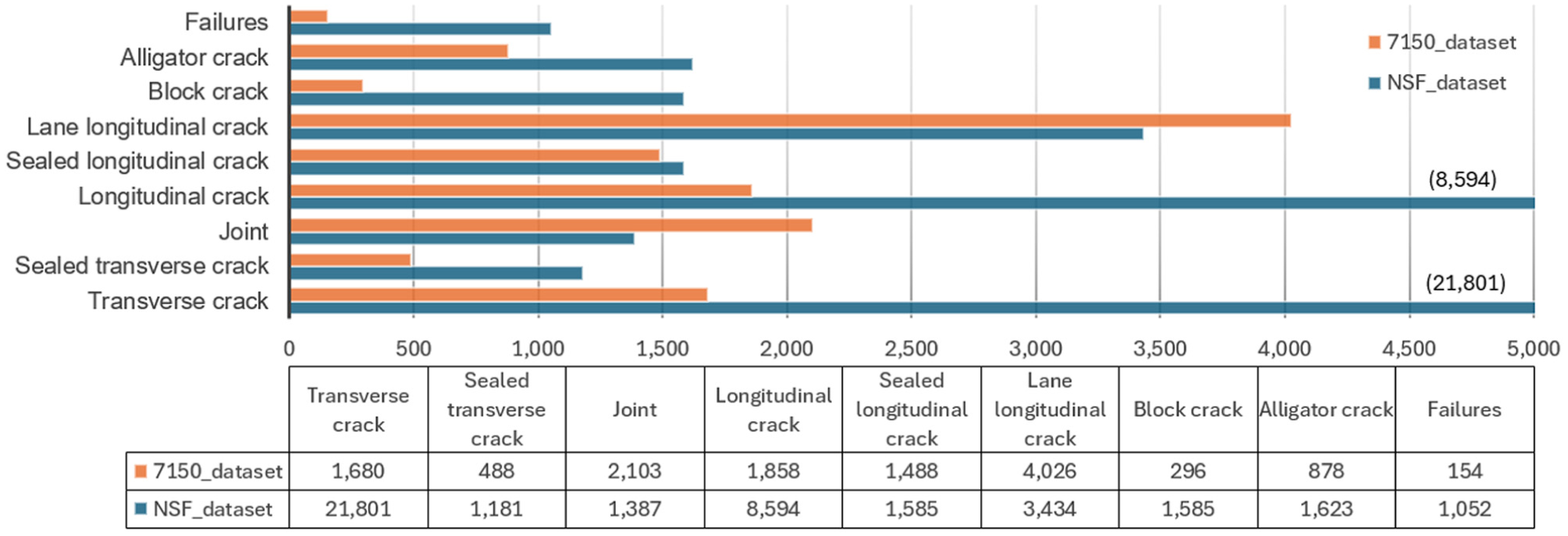
Instances of ACP pavement distress in two datasets.
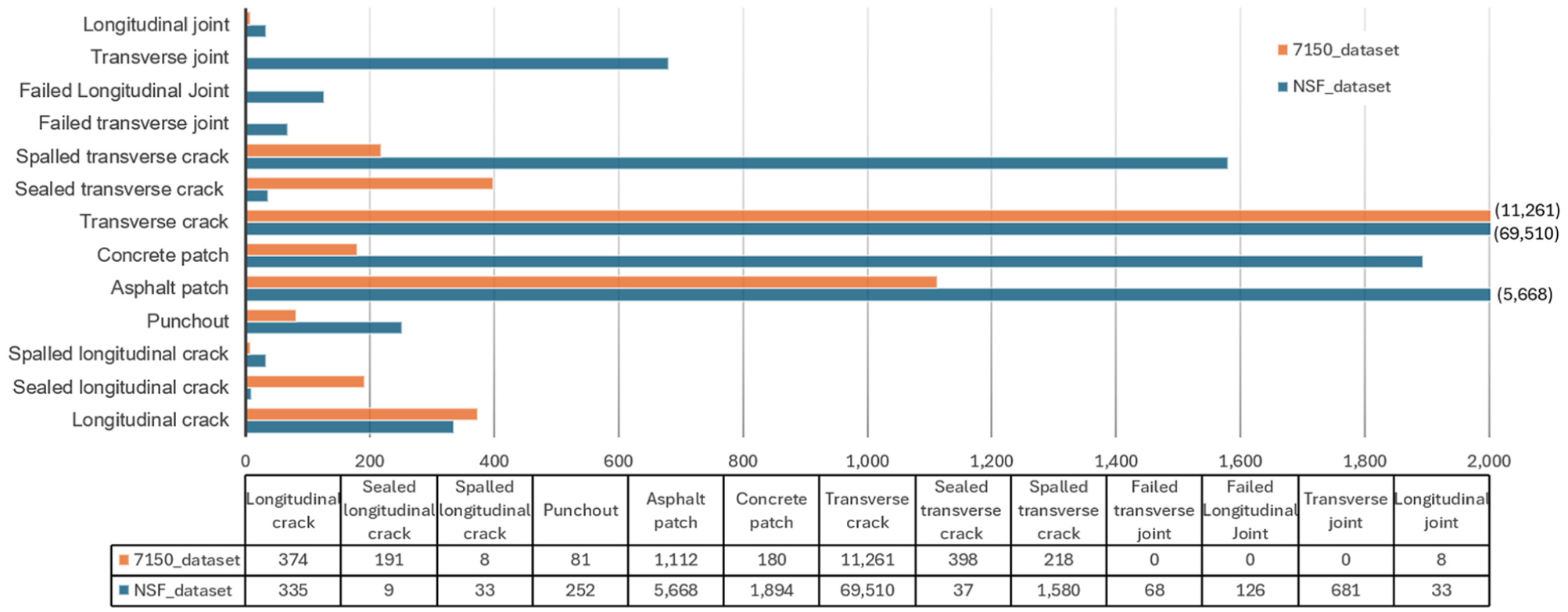
Instances of CRCP pavement distress in two datasets.
Data Split and Base Model Selection
For each dataset, 80% of images are used for training, with the remaining 20% reserved for validation and testing. This split is based on previous research ( 6 , 7 ) for 2D/3D image data of various pavements.
As shown in the Related Work section, many successful applications have been implemented for pavement distress detection using deep learning models and 2D/3D images. Because there have been previous successful applications with YOLOv11 ( 7 , 39), this paper utilizes YOLOv11, developed by Ultralytics ( 40 ), as a substantial leap forward in real time object detection, as the base model. Therefore, different strategies to refine and improve the base model’s performance with these two datasets can be evaluated.
Yolov11 employs more efficient modules (see Figure 4), including C3K2 blocks, Spatial Pyramid Pooling Fast, and advanced attention mechanisms such as Cross-Stage Partial with Self-Attention (C2PSA) ( 41 ). The versatility of YOLOv11 enables its application across various tasks, including object detection, instance segmentation, image classification, pose estimation, and object tracking ( 42 ). YOLOv11 focuses more on enhancing small object detection and overall accuracy while maintaining real time inference speeds. Its architecture and detailed explanations for each block’s abbreviation are shown in Figure 4. For feature extraction, the backbone introduces the C2PSA module using cross-stage partial networks with self-attention mechanisms. The extracted features are transformed and refined by the neck before passing them to the head to generate predictions for the input images.
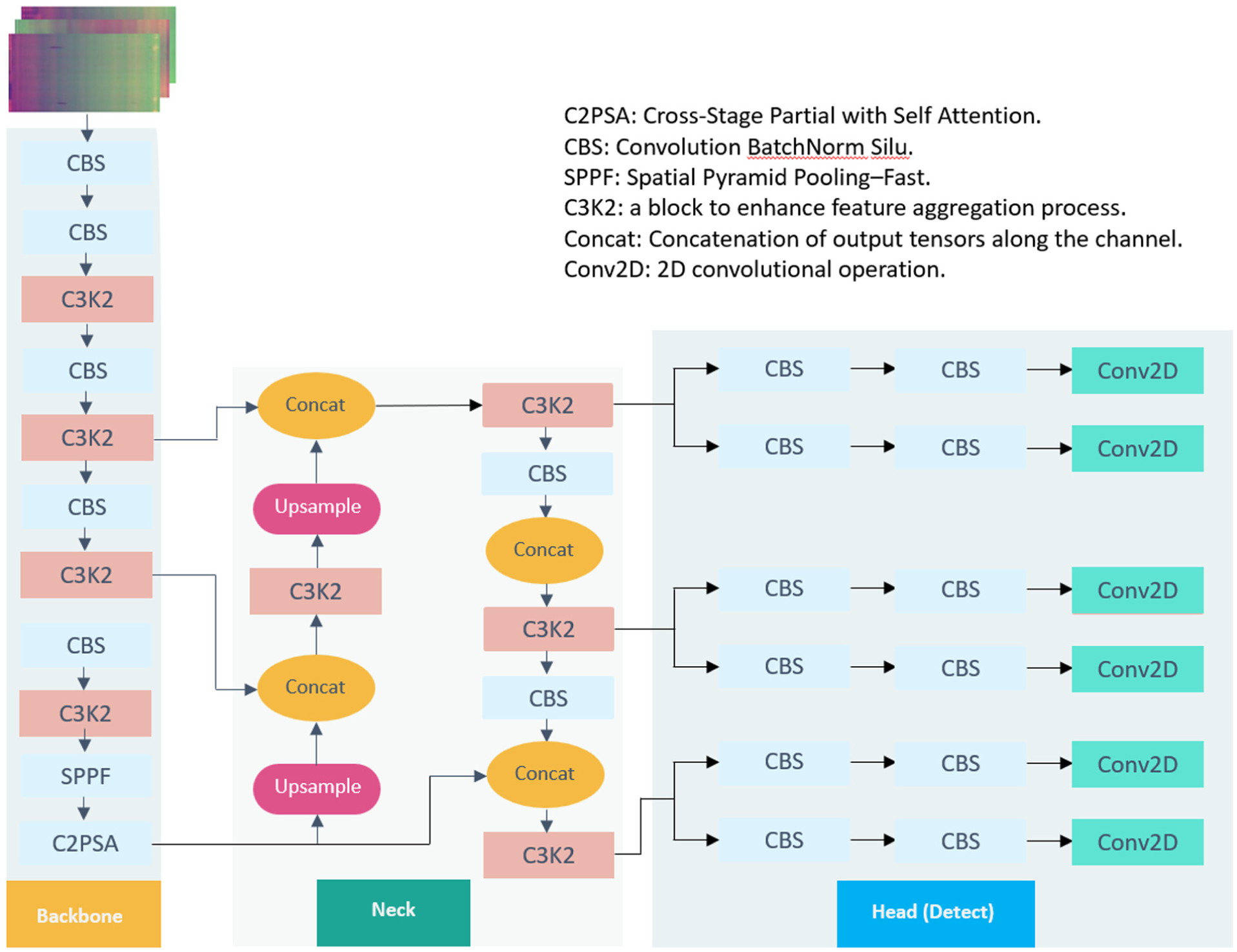
Architecture of YOLOv11.
In Yolov11, the Distribution Focal Loss function is employed to address class imbalance, building on the principles of the FL function ( 42 ). The latter magnifies the loss for underrepresented image examples and effectively forces the training to focus more on hard-to-classify examples. Therefore, the class imbalance in the datasets used in this paper can be mitigated.
Strategies that Can be Applied to Two Different Data Sources
Given two available datasets, several strategies for model adaptation, as shown in Figure 6, are tested. For the TL techniques, three primary approaches can be used for refining a new model with new datasets ( 43 ): (1) feature extraction using pretrained weights by excluding the final fully connected layer; (2) partial network freezing by retaining early-layer features; and (3) model fine-tuning with new datasets. The last two TL strategies are considered in this paper, which are the layer-frozen and fine-tuning (abbreviated as TL and FT in the names of model training scenarios in the Experiment section), respectively.
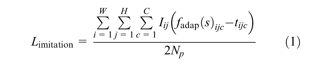
KD employs a dual-model framework consisting of a teacher model and a student model. The former, typically larger and more accurate, transfers its learned knowledge to the compact student model through a distillation process, as shown in Figure 5. This approach serves as a knowledge transfer mechanism and a model compression technique. For the YOLOv11 implementation, the fine-grained imitation method created by Wang et al. (
44
) is developed in this paper. The student model learns to replicate the teacher’s feature responses in regions near detectable objects, which are defined by a fine-grained imitation mask
where
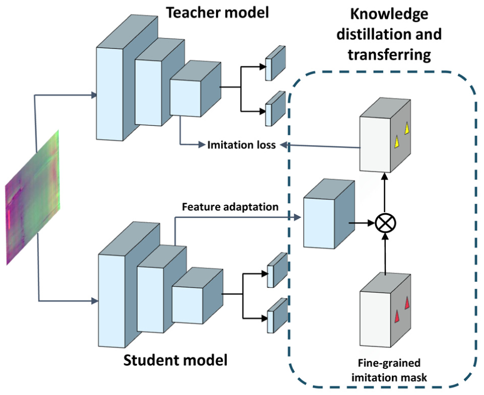
Knowledge distillation between two models.
The training loss is calculated by,

where
In this paper, these strategies are systematically implemented using YOLOv11 as the base model. First, the baseline models are created by fine-tuning separately on each dataset (Figure 6a) and on their combined version (Figure 6e). Then, the additional model variants are generated using: (1) fine-tuning of baseline models on another dataset (Figure 6b); (2) freezing a few initial layers (see Figure 6c. In this study, five layers are frozen); and (3) distilling knowledge between baseline models to determine a compact but robust student model (Figure 6d).
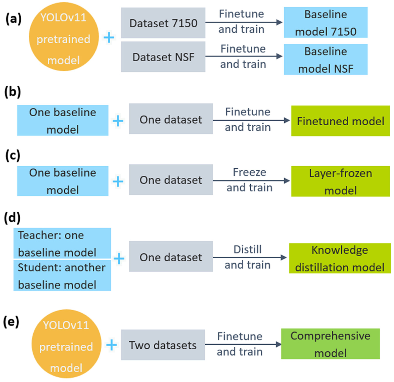
Strategies using two different pavement datasets: (a–c, and e) two TL strategies; and (d) shows how to use the KD strategy.
Metrics to Evaluate Models Trained with Different Strategies
To evaluate the performance of these trained models, several metrics are used. These selected metrics are the standard to measure the performance of object detection ( 41 ) and pavement distress detection ( 22 ).
Precision and Recall


where TP, FP, and FN represent true positive, false positive, and false negative, respectively.
Average Precision and mAP50
The precision-recall trade-off for one damage class can be defined by the average precision (AP) for how accurately predicted distress types and their bounding boxes are over the ground truth. It is calculated as the area under the precision-recall curve.

where
Mean average precision (mAP), especially mAP50 (mAP is at least 50%), is computed for the overlaid prediction and ground truth. This is how mAP50 is obtained.

where
The precision, recall, and mAP50 are in the range 0–1. For example, if the more correct predictions are made by a trained model on the validation or testing dataset, those metrics are closer to one. Otherwise, the three metrics could be very low and close to zero, which indicates the model fails to identify the defined pavement distresses.
Experiments
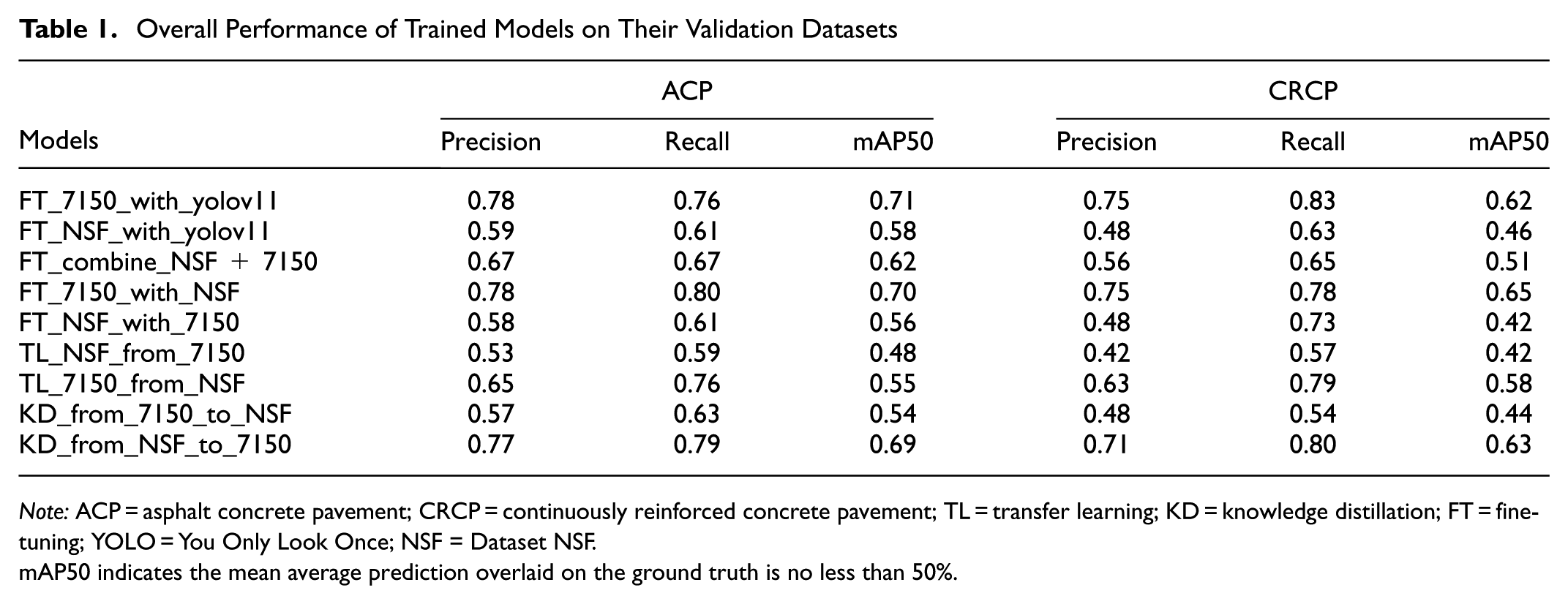
In this paper, an NVIDIA RTX A6000 is used as the Graphics Processing Unit (GPU) for training and testing. The hyperparameters of YOLOv11 are set as follows. The learning rate is in the range 0.00001–0.1, and the momentum is between 0.6 and 0.98. The optimizer is AdamW, the batch size is 16, and the drop rate is 0.15. In total, 1,000 epochs are defined to maximize GPU usage, but early stopping is activated during training. These hyperparameters remained unchanged in the following model training scenarios. The overall performance of these models is summarized in Table 1 and shown in Figures 7–12 for the ACP and CRCP datasets.
Overall Performance of Trained Models on Their Validation Datasets
Note: ACP = asphalt concrete pavement; CRCP = continuously reinforced concrete pavement; TL = transfer learning; KD = knowledge distillation; FT = fine-tuning; YOLO = You Only Look Once; NSF = Dataset NSF.
mAP50 indicates the mean average prediction overlaid on the ground truth is no less than 50%.
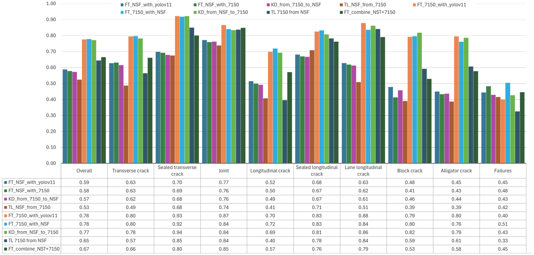
mAP50 of each trained model for ACP datasets.
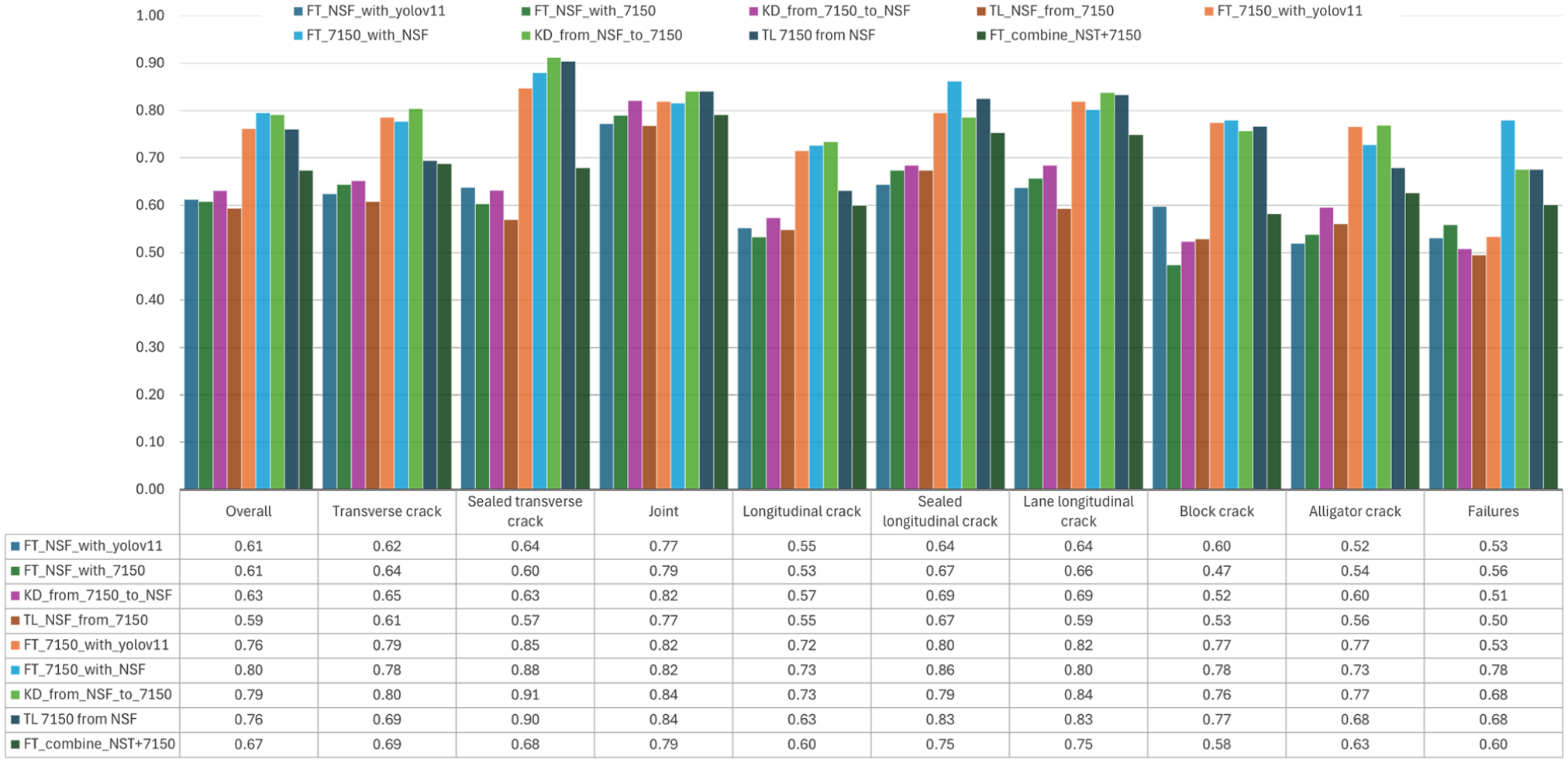
Precision of each trained model for ACP datasets.
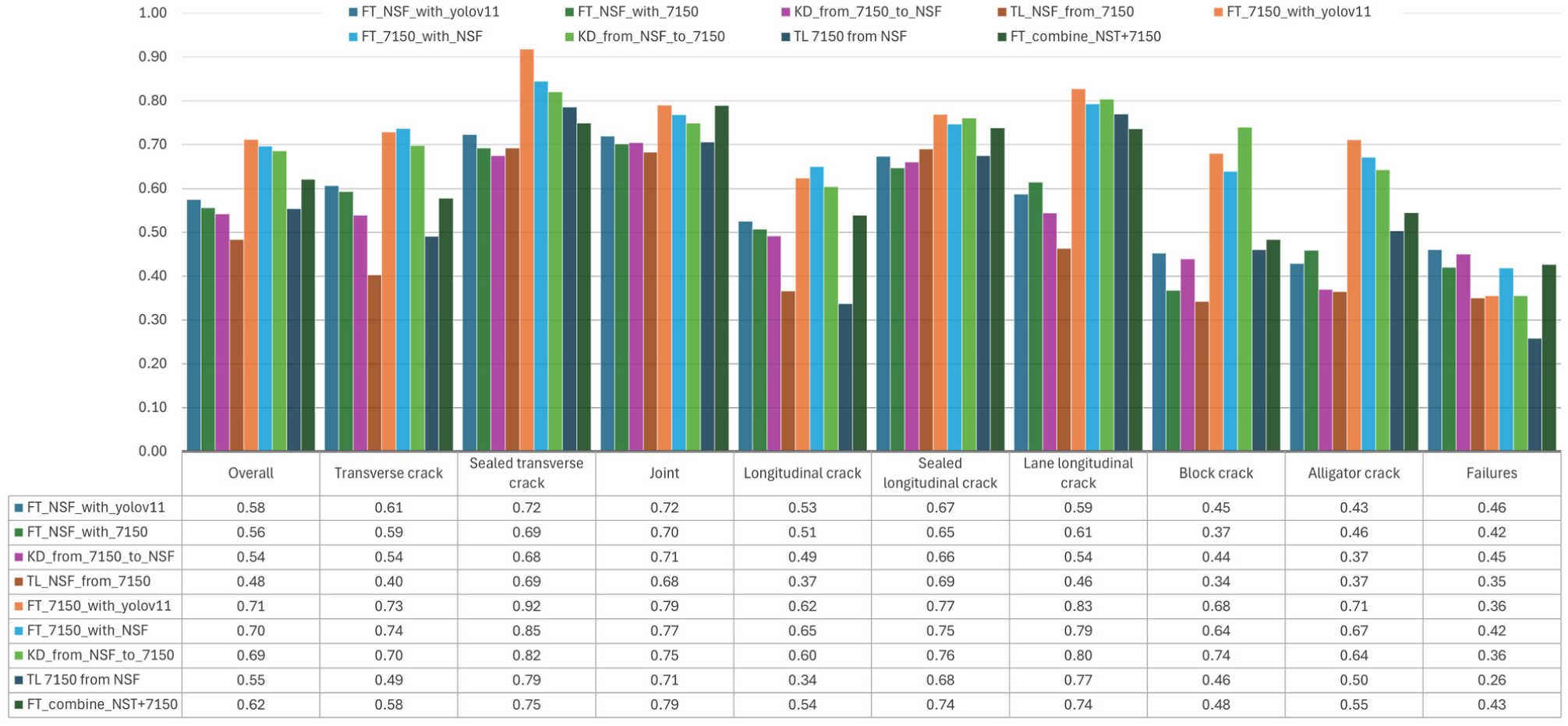
Recall of each trained model for ACP datasets.
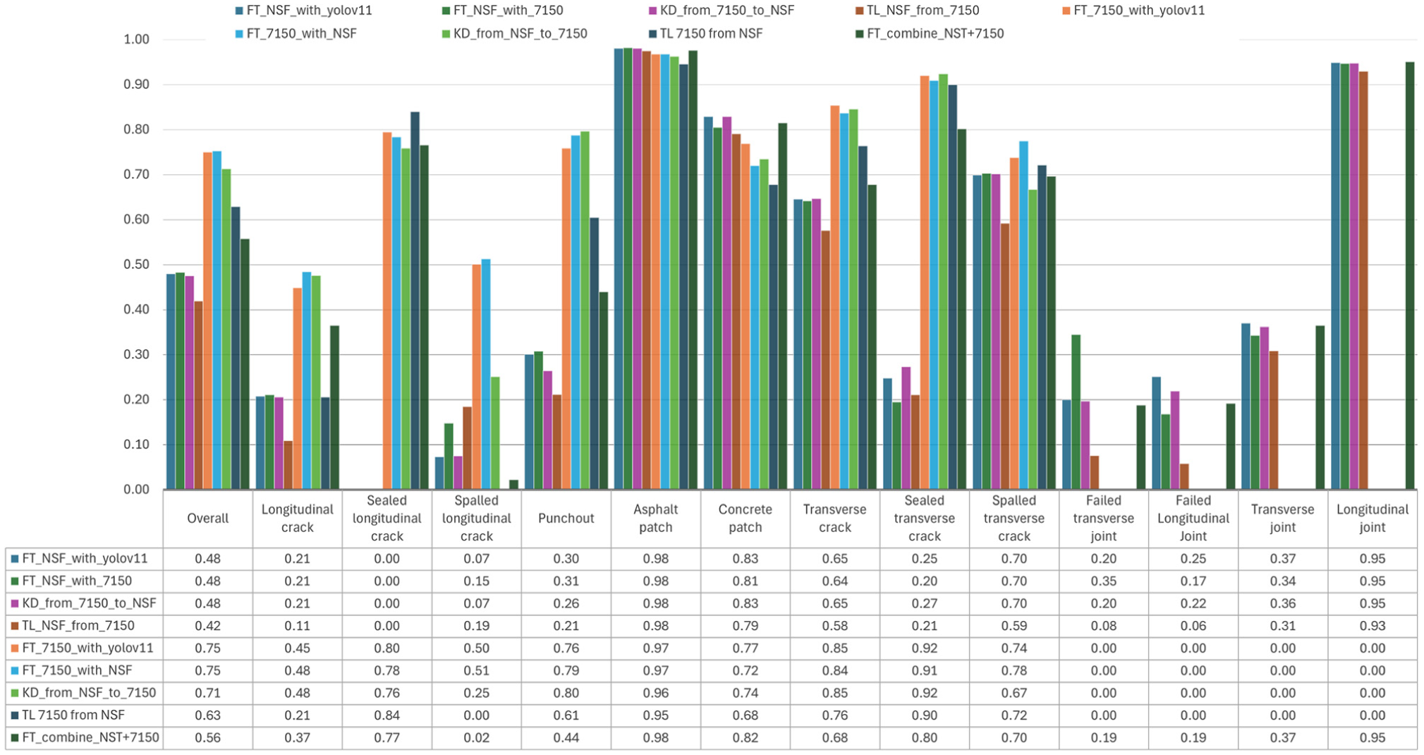
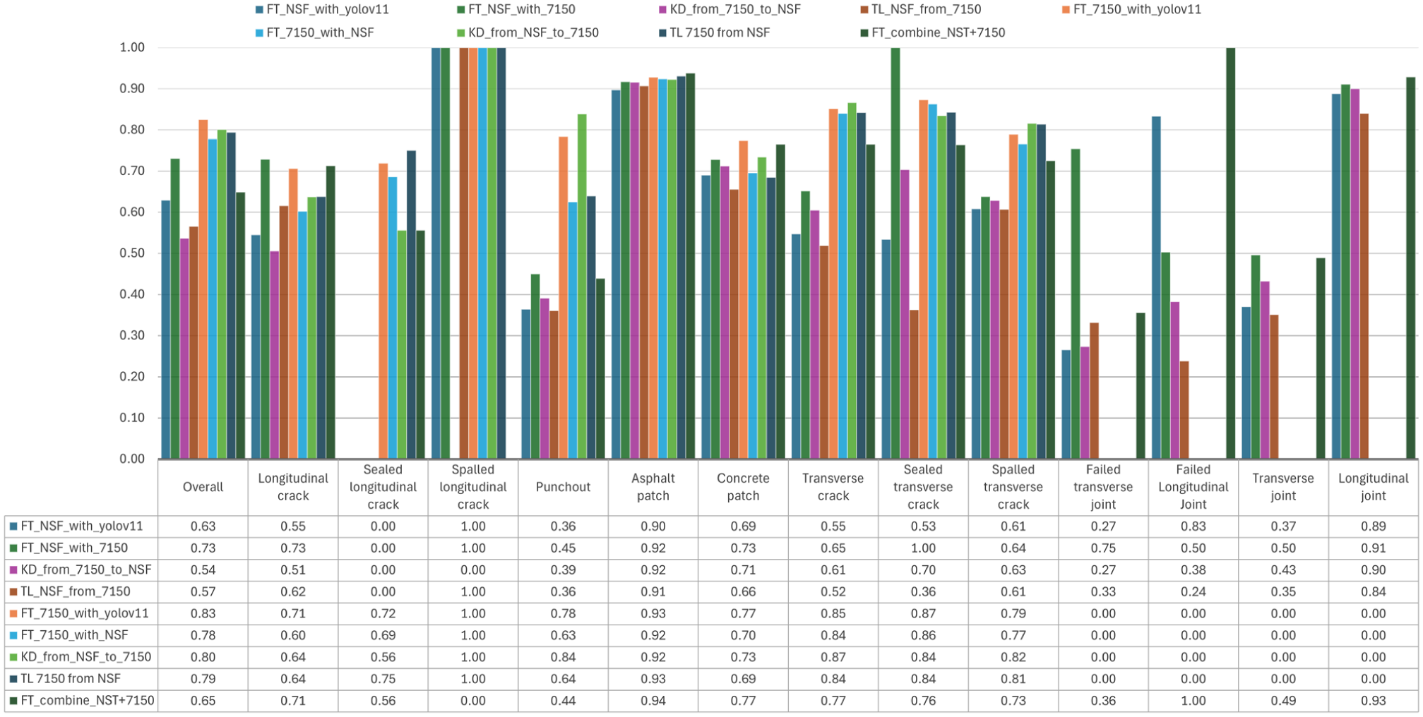
mAP50 of each trained model for CRCP datasets.
Precision of each trained model for CRCP datasets.
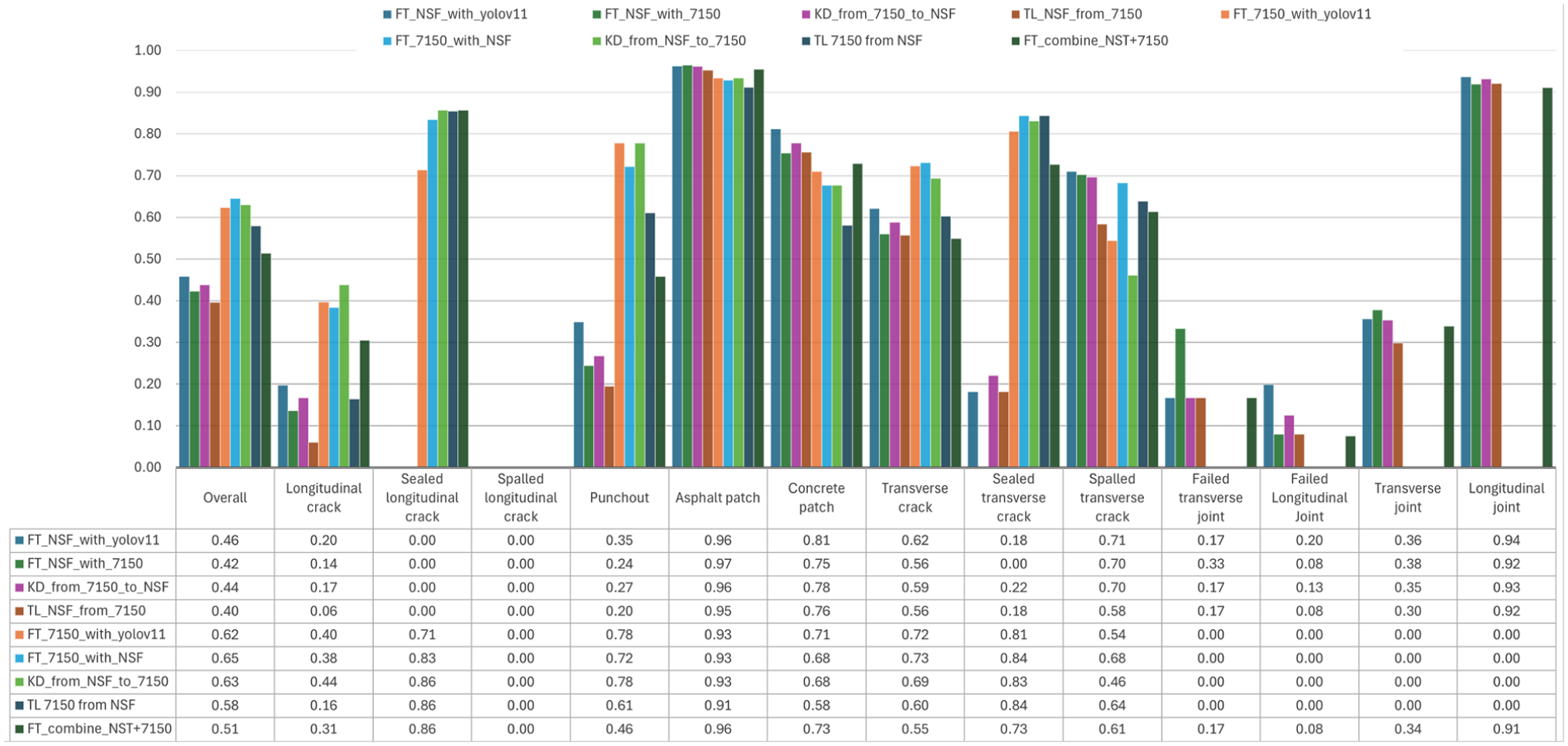
Recall of each trained model for CRCP datasets.
Model Training Scenarios
During the training process, all the fused 2D/3D images (right column in Figure 1) are resized to a uniform size of 1,024 × 1,024. The same data augmentation skills are employed for the ACP and CRCP datasets, although other image sizes tested in Gong et al. ( 6 ), Bai and Wang ( 7 ), and Sanchez ( 8 ) show limited effects on such training. The following training scenarios represent different strategies utilizing two different models and the baseline models.
FT_NSF_with_yolov11: YOLOv11 is used as the base model to train on Dataset NSF.
FT_NSF_with_7150: baseline model trained from Dataset 7150 is fine-tuned with Dataset NSF.
KD_from_7150_to_NSF: teacher and student models are baseline models trained from Datasets 7150 and NSF for the use of the KD strategy.
TL_NSF_from_7150: five initial layers of the baseline model trained from Dataset 7150 are frozen during the new training on Dataset NSF.
FT_7150_with_yolov11: YOLOv11 is used as the base model to train on Dataset 7150.
FT_7150_with_NSF: baseline model trained from Dataset NSF is fine-tuned with Dataset 7150.
KD_from_7150_to_NSF: teacher and student models are baseline models trained from Datasets NSF and 7150 for the use of KD.
TL_7150_from_NSF: five initial layers of the baseline model trained from Dataset NSF are frozen during the new training on Dataset 7150.
FT_combine_NSF + 7150: YOLOv11 model is fine-tuned with Datasets 7150 and NSF.
Performance Using Various Strategies to Train Deep Learning Models with ACP Datasets
Models are validated during training. The following are the results for the ACP datasets. Observations for CRCP are addressed in the following section.
Performance of mAP50 on ACP datasets: For the overall performance, Figure 7 and Table 1 indicate that fine-tuning the baseline model with alternated dataset training yields nearly identical mAP50 scores for the 7150 and NSF datasets. The KD between baseline models shows a small performance degradation. In contrast, the layer-frozen causes significant mAP50 reductions of 6% (Dataset NSF) and 15% (Dataset 7150) compared with the performance of baseline models. For rare distress such as failures, fine-tuning of the models trained on another dataset has an improvement. These results suggest that fine-tuning maintains model effectiveness across the two datasets; however, layer-freezing substantially compromises detection accuracy.
Performance of precision on ACP datasets: Fine-tuning and KD strategies show modest improvements in the overall precision; however, fine-tuning demonstrates consistent gains at overall and class-specific levels (see Figure 8 and Table 1). Meanwhile, the layer-frozen achieves comparable performance on training Dataset 7150, but results in a marginal decrease in precision for Dataset NSF. The FT_combine_NSF + 7150 model demonstrates the improvement over the models trained with the Dataset NSF.
Performance of recall on ACP datasets: Both fine-tuning and KD between baseline models result in small recall reductions to their overall performance. In contrast, the layer-frozen strategy leads to substantial recall declines of 10% and 6% for training on Datasets NSF and 7150, compared with the performance of their baseline models (Figure 9 and Table 1). The performance of the FT_combine_NSF + 7150 model is better than that of the models trained with the Dataset NSF.
When applied to the ACP datasets, the fine-tuning strategy consistently achieves comparable or superior performance metrics (mAP50, precision, and recall) compared with baseline models. In particular, this approach demonstrates the effectiveness for rare distress categories (e.g., failures), where performance can be improved at 11% in mAP50 (Figure 7), 25% for precision (Figure 8), and 6% for recall (Figure 9). These results suggest that the fine-tuning from the baseline model keeps general detection accuracy and is an effective countermeasure against class imbalance by increasing the number of examples for rare pavement distresses in pretrained models.
Performance Using Various Strategies to Train Deep Learning Models with CRCP Datasets
The validation datasets for CRCP show incomplete representation of certain distress classes. Dataset 7150 lacks joint distress examples, and there are no instances of sealed longitudinal cracks in Dataset NSF in the following analyses (see Figures 10 –12). The overall performance of these models on the validation datasets is given in Table 1.
Performance of mAP50 on CRCP datasets: In Figure 10 and Table 1, using the fine-tuning from the model trained by Dataset 7150 on Dataset NSF gains the highest mAP50, but the KD and layer-frozen cause a decline at different levels, for the model’s performance. However, the FT_combine_NSF + 7150 model shows its versatility for each distress, indicating that more training examples are key to improving the mAP of automated pavement distress detection.
Performance of precision on CRCP datasets: For the overall precision of these models, as shown in Figure 11 and Table 1, fine-tuning the model trained by Dataset 7150 on the NSF dataset improves the precision by up to 10%. However, the KD and layer-frozen cause declines of 9% and 6%, respectively. The combined dataset improves the performance of the fine-tuned models on individual and rare distress, such as various joints.
Performance of recall on CRCP datasets (recall): The overall recall slightly decreases when applying KD, fine-tuning, and layer-frozen strategies on the training using Dataset NSF (Figure 12 and Table 1). In contrast, the fine-tuning and KD strategies increase recall for training on Dataset 7150 marginally because the layer-frozen causes a decline of 4%. The FT_combine_NSF + 7150 model increases recall when testing on rare distress types.
There are two findings from this paper. First, fine-tuning a baseline model consistently enhances the performance of a newly trained model. Second, the comprehensive model trained on two datasets indicates an average performance for the individual baseline models. The models’ generalization capabilities are examined in the following section.
Cross-Validation to Evaluate the Generalization of Trained Models
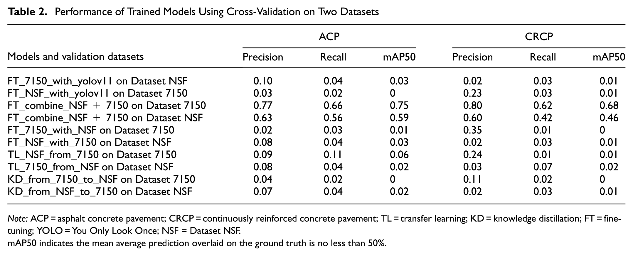
To answer the question of how the fine-tuned or distilled models perform after being trained on new datasets using the proposed strategies, a cross-validation study was conducted in this paper. Table 2 presents the comparative performance of models trained on different datasets and validated against datasets prepared to train the baseline models.
Performance of Trained Models Using Cross-Validation on Two Datasets
Note: ACP = asphalt concrete pavement; CRCP = continuously reinforced concrete pavement; TL = transfer learning; KD = knowledge distillation; FT = fine-tuning; YOLO = You Only Look Once; NSF = Dataset NSF.
mAP50 indicates the mean average prediction overlaid on the ground truth is no less than 50%.
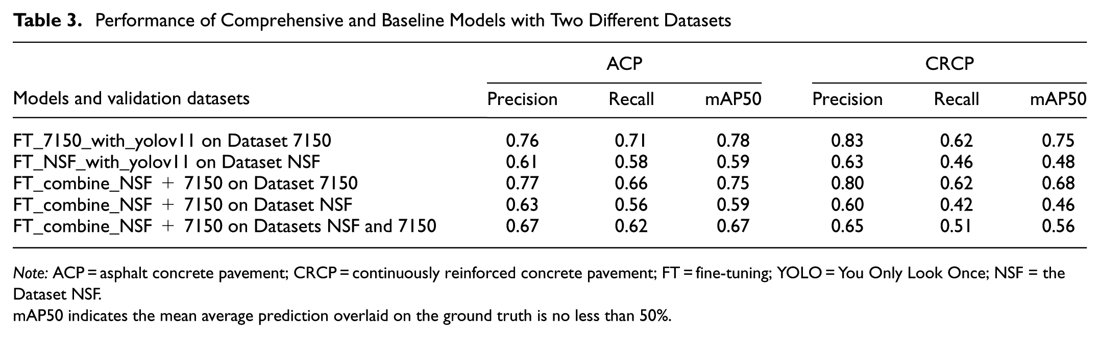
The findings reveal that models refined using the fine-tuning, KD, or layer-frozen with a new dataset cause severe performance degradation when applied to previous training datasets, achieving near-zero scores in precision, recall, and mAP50 during cross-validation. However, the comprehensive model achieves a comparable overall performance to baseline models over the same validation dataset, although its performance is at an average level on the combined validation dataset compared with the baseline models trained by individual datasets, as indicated in Table 3. Therefore, the two datasets should be merged and used for the fine-tuning of a new model.
Performance of Comprehensive and Baseline Models with Two Different Datasets
Note: ACP = asphalt concrete pavement; CRCP = continuously reinforced concrete pavement; FT = fine-tuning; YOLO = You Only Look Once; NSF = the Dataset NSF.
mAP50 indicates the mean average prediction overlaid on the ground truth is no less than 50%.
Computational Cost for Different Strategies
Computational costs vary when the different training strategies are used (Table 4). The KD requires much more training time per epoch than the fine-tuning and layer-frozen methods, although the number of parameters is the same. For the inference, the KD processes one image at 3.05 ms and 2.15 ms, respectively, for the ACP and CRCP datasets. The other two methods can achieve 1.25 ms per image on these datasets. This difference persists, although KD should yield fewer parameters after pruning the teacher models. However, this paper evaluates fine-grained KD, and the findings do not preclude the effectiveness of other KD methods.
Number of Parameters and Average Time Using Different Strategies During Training and Inference
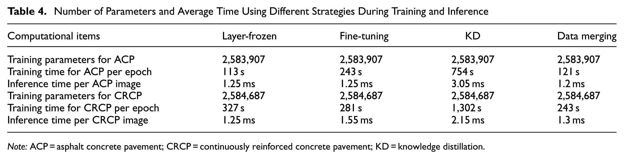
Note: ACP = asphalt concrete pavement; CRCP = continuously reinforced concrete pavement; KD = knowledge distillation.
Discussion
In this paper, two datasets collected from different vendors are selected and annotated using in-house tools. These datasets are different because of variations in data collection hardware, sensor resolutions, road conditions, data collection timelines, and annotation quality. Metrics such as mAP50, precision, and recall are used to evaluate the models’ performance on validation and cross-validation datasets (Tables 1 and 2 and Figures 7–12) for all strategies on different pavement types. Two TL strategies are thoroughly explored. The fine-tuning, in particular, proves effective in training a new model using base models like YOLOv11, and the fine-tuning proves that it is more capable of transferring knowledge from a pretrained model to a new one. The focus of this paper was to detect different pavement distresses automatically on different pavement types using deep learning methods and strategies. In the future, the best-trained models will be integrated into the automated road surface condition evaluation framework for state-wide applications.
This paper shows that the performance of current trained models is heavily constrained by dataset limitations. These limitations primarily include distress type imbalance, especially the underrepresentation of certain distresses, and poor cross-domain generalization. As described in the Experiment section, these annotated datasets differ in resolution and sources and in the distribution of distress types. For example, Dataset NSF contains more critical distress cases, such as transverse cracks, than Dataset 7150 for ACP and CRCP datasets. This imbalance shows certain effects on the training and causes inconsistent performance with the proposed strategies. Currently, imbalance-aware training techniques, including but not limited to weighted losses, FL variants, or oversampling of rare classes, are conducted in ongoing projects. Factors such as distress severity, sample size threshold, and model architecture should be studied carefully to address the distress imbalance problem. In addition, to overcome these challenges, targeted data collection could be a viable solution for enhancing the robustness and generalization of pavement distress detection.
However, KD is traditionally employed to transfer knowledge from a larger, more complex teacher model to a smaller, lighter student model, aiming to compress model size while retaining performance. However, in this paper, KD is applied from a teacher model trained on either Dataset 7150 or NSF to a student model trained on either Dataset NSF or Dataset 7150. Both teacher and student models are based on the same YOLOv11 architecture and a similar dataset size. As shown in previous sections, the results indicate that KD did not yield performance gains over the fine-tuning and layer-frozen strategies. In addition, the computational cost of the KD is much higher than that of the other two methods. Future research should be focused on exploring alternative KD techniques or integrating them with domain adaptation methods for potential performance improvement.
In addition, because the individual datasets were prepared for different projects with distinct objectives, a decision must be made between developing a unified approach for both and retaining the original single-dataset setting. Although each data set could be expanded using additional costly manual annotation, these efforts can only benefit the data scanned from the same data vendor, regardless of model performance. This limitation can be addressed via the implementation of more advanced strategies of model training to find the solution.
Conclusions
An investigation of how to leverage deep learning strategies was implemented in this paper when working with multiple, heterogeneous 2D/3D image datasets for pavement surface distress. Comprehensive experiments were conducted on labeled ACP and CRCP datasets, comparing four practical approaches, including fine-tuning a baseline model, freezing a few initial layers of a baseline model, distilling knowledge from domain-specific pretrained models, and refining a comprehensive model by integrating two distinctive datasets. This research involves rigorous performance evaluation using multi-metric assessment and cross-validation protocols to determine the most effective strategy for the effective use of two available image datasets collected from different data sources (vendors). The following are the findings in this paper.
The fine-tuning based on a pavement-specific baseline model outperforms the use of generic YOLO base models when using one dataset to train, indicating that the domain-relevant pretraining enhances the performance of a deep learning model even when datasets come from different sources (vendors). This confirms that TL improves pavement defect identification across datasets.
The comprehensive model, trained by mixing two different datasets, is the most generalized and robust model applicable to both pavement datasets based on cross-validation results. To increase the model’s generalization capabilities, more diverse data is critical to train deep learning models for pavement condition evaluation.
From this paper, data merging is recommended to handle two different datasets for automated pavement distress detection and condition evaluation.
In future research, the development of efficient deep learning frameworks (see the Discussion section), including other KD techniques, will be a focus, along with increasing the number of examples of rare distresses to further improve the accuracy and robustness of automated pavement distress detection models.
Footnotes
Acknowledgements
We really appreciate the reviewers of the 2026 TRB Annual Meeting for their constructive insights and suggestions on this paper.
Author Contributions
The authors confirm contribution to the paper as follows: study conception and design: Yongsheng Bai; data collection: Yongsheng Bai, Haitao Gong; analysis and interpretation of results: Yongsheng Bai, Haitao Gong; draft manuscript preparation: Yongsheng Bai. All authors reviewed the results and approved the final version of the manuscript.
Declaration of Conflicting Interests
The authors declared no potential conflicts of interest with respect to the research, authorship, and/or publication of this article.
Funding
The authors disclosed receipt of the following financial support for the research, authorship, and/or publication of this article: This study is funded by the US National Science Foundation (Grant number 2213694) and the Texas Department of Transportation (Project number 0-7150).

Any opinions, findings, conclusions, or recommendations expressed in this paper are those of the authors and do not necessarily reflect the views of the National Science Foundation and Texas Department of Transportation.