






Abstract
Ground-penetrating radar (GPR) has been used for nondestructive evaluation of hot-mix asphalt (HMA) pavements including density prediction. HMA density is an acceptance quality characteristic (AQC) used across the U.S. AQCs are the basis for quality control and acceptance, and are used by agencies to determine contractors’ pay. Recently, roller-mounted GPR was introduced to monitor HMA density in real-time, enabling roller operators to make more informed decisions to avoid under- and over-compaction of HMA layers. In this study, a Markov decision process (MDP) is formulated to represent the rolling pattern optimization problem. This formulation accounts for GPR prediction error, density spatial variability, and uncertainty in density progression. The introduced MDP provides contractors and roller operators with a tool to minimize operational costs while achieving target density, thereby enhancing pavement service life and reducing maintenance activities. Data collected from several field projects were used in the MDP formulation. The benefits of using the developed MDP for compaction decisions were demonstrated using project data from Illinois, U.S. The analysis was conducted for an actual project scenario under Illinois’ quality control for performance (QCP) program and was extended to a hypothetical pay for performance (PFP) scenario to evaluate the generalizability of the approach under different risk levels. Compared with an experienced roller operator, MDP decisions reduced the construction time by 40.3% and 18.1% and increased the revenue by 9.7% and 50.2% for the QCP and PFP scenarios, respectively. Additional benefits in energy savings, reduced construction-related delays, and improved worker safety are expected.
Keywords
Introduction
State highway agencies (SHAs) use various programs to accept products delivered by contractors. One product of interest to this study is hot-mix asphalt (HMA). Illinois Department of Transportation (IDOT) in the U.S. developed two HMA performance-related acceptance programs: quality control for performance (QCP) and pay for performance (PFP). QCP specifications are usually applied to smaller projects with 1,200 to 8,000 tons of HMA, whereas PFP specifications are applied to larger projects with 8,000 tons or more of HMA ( 1 , 2 ). The goal of these acceptance programs is to improve the long-term performance of pavements, which, in turn, reduces costly maintenance and rehabilitation activities.
Agencies use acceptance quality characteristics (AQCs) for determining the product’s acceptability ( 3 ). SHAs also use some AQCs to determine the contractor’s pay adjustment. AQCs are divided into two categories: materials and construction. Materials AQCs, such as air voids (AV) and voids in mineral aggregate (VMA), are measured from plant- or field-sampled mixes, either loose or laboratory-compacted. Construction AQCs, such as mat density and ride quality, are measured from the compacted mat ( 4 ). A contractor’s pay adjustment is usually a weighted combination of both material and construction AQCs results. In Illinois, a composite pay factor (CPF) including AV, VMA, and mat density, with weights 0.3, 0.3, and 0.4, respectively, is used ( 5 ). The contractor’s adjusted pay is calculated by simply multiplying the CPF by the contracted amount.
For accepted HMA products, contractor’s pay adjustment could be an incentive (bonus, CPF > 1) in the case of superior product quality, a disincentive (penalty, CPF < 1) in the case of inferior quality, or full pay (CPF = 1). However, in the case of unaccepted product quality, the contractor might face monetary deductions up to the contracted amount (no pay). In other cases, the contractor may be even asked to remove, or remove and replace, the unaccepted constructed material. Disincentives are a major concern for contractors: in the years 2015 and 2016, 55% of QCP projects and 44% of PFP projects in Illinois were penalized ( 6 ). These penalties averaged around $20,000 per project ( 6 ).
Contractors are also required to monitor the quality of their own product; this is usually referred to as quality control (QC). QC practices help the contractor assess and adjust their production and construction practices directly at the plant or on site to meet specifications. QC results serve as reference in disputes when conflicting results are reported. Conflicting results may be a result of differences in sampling, testing, material, and/or construction variability ( 7 ). For the Illinois data collected in the period 2015–2016, 196 mixes were disputed ( 6 ). This is largely because of HMA’s inhomogeneity and the agency’s random spot checks.
HMA mat density is reported to be an AQC in all states of the U.S. ( 4 ). This is because density is a key indicator for HMA short- and long-term performance ( 8 ). Under-compacted HMA is subjected to oxidation or accelerated ageing, moisture damage, fatigue cracking, and early-life rutting ( 9 – 13 ). Over-compacted HMA is subjected to other pavement distresses such as bleeding ( 12 ). Therefore, real-time monitoring of HMA density during compaction ensures meeting target density range. In Illinois, in the period 2015–2017, mat density was the main AQC driving contractor disincentives in both QCP and PFP specifications ( 14 ).
Conventionally, to determine the rolling pattern, contractors either rely on their experience or construct control strips at the beginning of relatively large projects. The strips are compacted by rollers, and density is sparsely monitored using nuclear gauges after each roller pass ( 15 ). The resulting density progression curve is used to find an optimum number of roller passes. Nuclear gauge measurements must be calibrated against ground-truth cores. Mat density is dependent on several factors including roller characteristics (e.g., weight, vibration frequency and amplitude), mix compaction temperature, ambient conditions, lift thickness, and underlying support ( 13 ). Most of these parameters are variable from one segment to another. Thus, a control strip density growth curve might not be representative of the required compaction effort for the whole project.
Coring serves as the ground truth measurement for HMA density. However, it is performed in sparse locations and post-compaction. Intelligent compaction reports intelligent compaction measurement values, which are correlated to HMA density, but have relatively low accuracy because of dependence on mix temperature and moisture content, and underlying layer stiffness and thickness, among other factors ( 16 ). Although compaction monitoring systems monitor mat temperature using infrared sensors, and number of passes using Global Positioning System (GPS), it may not be directly applicable for HMA density monitoring ( 17 ).
Ground-penetrating radar (GPR) may be used for real-time HMA compaction monitoring. It is a nondestructive device that emits low-energy electromagnetic (EM) waves. GPR signals are reflected when materials with different dielectric properties are encountered. The reflected signals are recorded and analyzed to infer material properties. One main property predicted using GPR signals is the dielectric constant or relative permittivity. The dielectric constant measures a material’s ability to store electrical energy when subjected to an external electric field ( 18 ). EM wave propagation speed and amplitude are affected by the dielectric constant of the medium material. GPR, coupled with signal processing techniques, can provide valuable information about pavement surface and subsurface, such as measuring pavement layers’ thicknesses, locating utility pipes, monitoring pavement density, and estimating moisture content ( 19 – 24 ).
EM waves are not affected by HMA temperatures ( 25 ). This allows the use of GPR technology during compaction while HMA cools down without the need for thermal sensors or temperature corrections. GPR may be mounted directly on roller compactors during HMA compaction ( 26 ). In a recent study, GPR was mounted directly on a roller compactor and was used to predict density progression curves for six different test sections ( 27 ). The final predicted HMA densities were validated using extracted cores, showcasing potential for advanced QC. Reporting HMA density should be followed by real-time decision-making to avoid under- and over-compaction based on the agency’s specified density limits. Moreover, compaction operational costs may be another limiting factor for extended rolling.
Technical Background
GPR Signal Processing
Signal processing steps may be applied to raw GPR signals for HMA density prediction. These steps include preprocessing for zero offset removal, signal instability, and height corrections ( 28 ). Other corrections, such as the removal of surface moisture and correction for thin layers, may be utilized (29–31). After signal corrections, the HMA dielectric constant can be estimated using Equation 1:
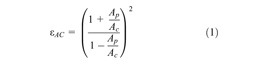
where
Afterwards, the Al-Qadi Lahouar Leng (ALL) density prediction model (Equation 2) may be used to predict pavement density ( 21 ). ALL density prediction model is derived from Bottcher dielectric mixing theory and has been recently updated by changing its shape and polarization factors ( 27 , 32 ). According to the dielectric mixing theory, the dielectric constant of a mix is a function of the dielectric constants and volumetric properties of its components ( 33 ).
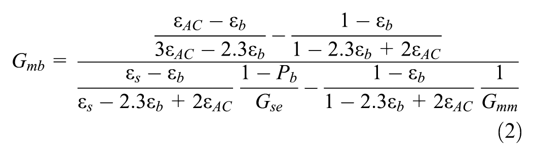
where
Markov Decision Process
Markov decision process (MDP) is a mathematical model for sequential decision-making problems when outcomes are uncertain ( 35 ). The name Markov highlights that MDPs follow the Markov property (memoryless property), where the future is conditionally independent of the past, given knowledge of the present, as modeled in Markov chains.
An MDP is usually defined for a discrete-time problem, with either finite (
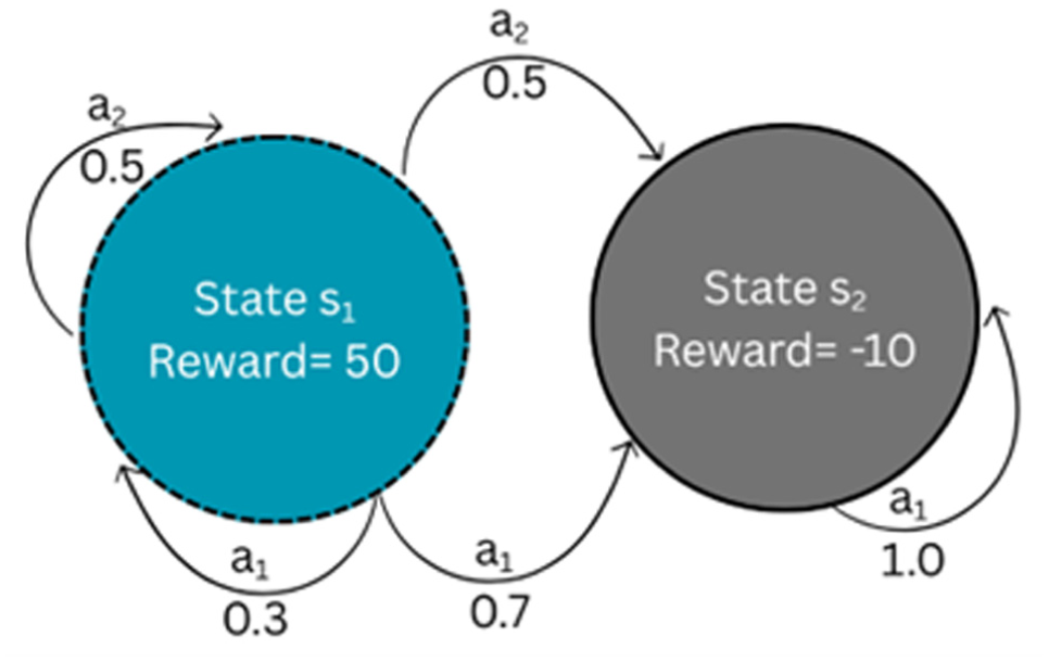
Schematic of a two-state Markov decision process.Note: a1 = action 1; a2 = action 2; s1 = state 1; s2 = state 2.
Solving an MDP means finding an optimal sequence of actions or an optimal “policy.” The optimal action is found by maximizing the total reward, which is the sum of immediate rewards and all expected future rewards. This expected total reward is often referred to as “utility” and is computed by solving Bellman’s equation (Equation 3).

where
Considering a finite decision horizon with N states, Bellman’s equation is, in fact, a system of N nonlinear equations and has no closed-form solution. Instead, iterative procedures may be used to find the optimal solution. The solution may be found using backward induction (usually for simple finite horizon problems), policy evaluation, or value iteration (
35
). Value iteration, first introduced by Shapley in 1953 for stochastic games, starts with an estimated value of 0 for all state utilities (

MDPs have been applied to several transportation optimization and planning cases (38– 41 ). In this paper, an MDP is used for optimizing the rolling pattern during compaction of HMA pavements. The goal is to help contractors achieve target density with minimal operational costs. HMA density progression curves obtained from roller-mounted GPR are used as input into MDP for real-time decision-making. The MDP formulation is discussed in detail in the next section.
MDP Formulation for Rolling Pattern
The rolling pattern is formulated as an MDP by specifying the problem-specific elements of the previously introduced framework: the state space (S), transition probabilities (P), action space (A), and reward function (R).The following observations were made about the rolling pattern by visiting several field projects in Illinois:
Each lane is divided longitudinally into segments. This is because of transporting HMA in batches using trucks, paver and crew productivity, and the need to maintain high material temperature during paving and compaction. An average segment length of 220 ft (67 m) was reported, depending on lift thickness, available crew and equipment, and project schedule. Figure 2 shows lane 3 from a field project around Bourbonnais, IL, with four longitudinal segments.
Roller operators divide the lane into sections transversely (sub-lanes), depending on their experience and the roller’s width. A typical tandem roller, used for main lane compaction, has a drum width around 60–80 in. (1.5-2 m) (lane width is 132–144 in. [3.3–3.7 m]). Therefore, some operators divide the lane into two sub-lanes and others divide it into three; the latter was observed to be more common. Figure 2 shows the sub-lane division (left, middle, and right).
There are several parameters that roller operators could control to change compaction effort. Commercial rollers have a range of vibration frequencies and amplitudes. Roller speed is in the rang 3–7 mph (4.7–11.2 km/h); an average speed of 4.4 mph (7.2 km/h) was observed. The number of roller passes depends on number of available rollers; with approximately 25 passes per segment (e.g., 9 for breakdown roller, 9 for intermediate roller, and 7 for finishing roller). Figure 2 shows about 10 passes/segment by the finishing roller moving in the east-west direction.
The density progression curve generally has an increasing trend with the number of passes until it reaches a plateau, and may decrease after a peak, reflecting a “locking” point. The trend may be represented by a parabolic or a logarithmic formula. Figure 3 shows an example progression curve from the same project.
A previous full-scale laboratory experiment estimated the GPR prediction error relative to extracted cores to be ±0.7% ( 27 ). This error was incorporated into the MDP formulation to represent density uncertainty in the expected agency rewards. The laboratory dataset was also used to evaluate and compare candidate transition models, as described later in this section.
GPR data from four field projects across Illinois—Kankakee, South Holland, Gilman, and Bourbonnais—were used during model development and testing. Data from the first three projects informed the estimation of spatial variability in density measurements for use in the rewards estimation. The Bourbonnais dataset was subsequently used to test the performance of the developed MDP.
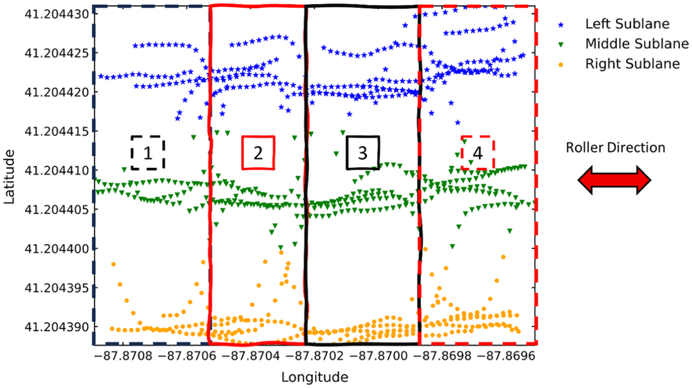
Finishing roller rolling pattern using Global Positioning System (GPS) data on a field project in Bourbonnais, IL.
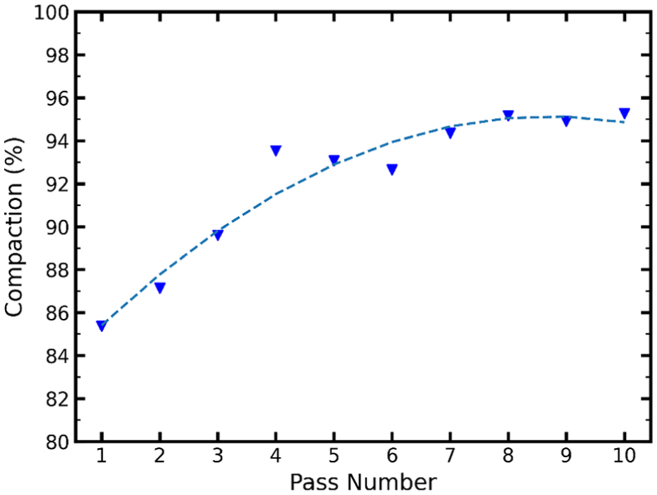
Example progression curve from lane 5, segment 2, middle sub-lane, with a parabolic fit.
States
Intuitively, for rolling patterns, the state should indicate the achieved density. However, two challenges arise: 1) the range of possible densities is large (70%–98% of
To overcome these challenges, the states are defined as tuples of the integer densities of three passes including the current pass; for example, the tuple (85, 87, 90) is the state reached after three passes with measured densities of 85%, 87%, and 90%. The decision to use three density values for state definition was a direct result of the chosen transition model as will be discussed later. States are defined for densities
Actions
The roller operator can change many parameters (e.g., vibration frequency, amplitude, and roller speed). However, the focus in this paper is the number of passes. Therefore, the possible actions at each state are to continue (perform one more pass) or to stop compaction:
Transition Probabilities
The large state space means that transition probabilities must be estimated parametrically, using a model fitting the different progression curves. The model estimates
For the 1-point & slope linear regression, the goal was to investigate the feasibility of incorporating laboratory data to predict field compaction. Dynamic time warping (DTW) and derivative dynamic time warping (DDTW) were used to evaluate the similarity between laboratory gyratory compaction curves and field roller compaction curves for the same mixes. In these approaches, the time axis is warped to identify similarities between the two series: either in values (in the case of DTW), or in slopes (in the case of DDTW). DDTW analysis showed a moderate average similarity value of 11. Therefore, the slopes from laboratory gyratory compaction curves were used to predict the corresponding field compaction curves.
The four models were evaluated in predicting future densities, and their mean absolute error results were 1.08, 1.86, 1.10, and 6.84 for the 3-point linear, 4-point parabolic, 1-point & slope linear, and 4-point B-spline models, respectively. An example of the prediction errors is shown in Figure 4. The 3-point linear model requires three observations before the initial prediction, and four observations for the 4-point parabolic, and so on. The 3-point linear model was chosen as the transition model because the model is simple, and allows skipping laboratory input without compromising prediction accuracy. Additionally, it is not expected to make early decisions in the first three passes.
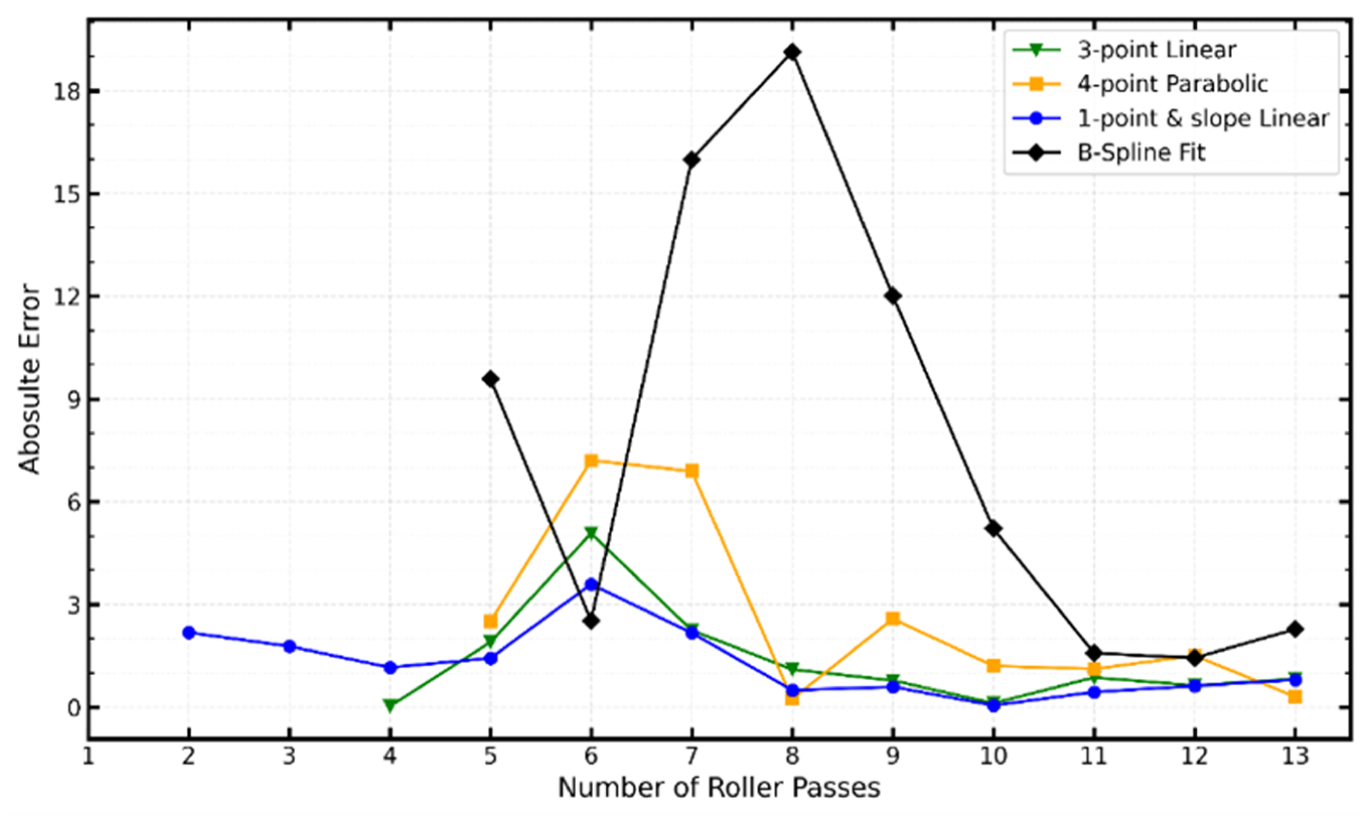
Example performance of the transition models on the left sub-lane of section A ( 27 ).
Although a linear model mathematically requires only two points, the GPR sensor in this study was mounted on one side of the roller. As a result, two consecutive measurements may have no meaningful change in density, making a 2-step definition less reliable for capturing actual progression. Including a third point allowed the model to better capture the compaction trend while maintaining early decision capability.
After choosing the transition model, a normal distribution was fitted to its prediction errors, as shown in Figure 5. The distribution of errors has a standard deviation (SD) of 1.5, which may be used as a default value to calculate the transition probabilities. For example, if the transition model predicts the next density to be 94.2%, a normal distribution of mean = 94.2 and SD = 1.5 (default) is used to calculate the transition probability from the current state to the state with density 95% by calculating the area under the normal PDF for the range 94.5%–95.4%, and similarly for all the other possible transitions.
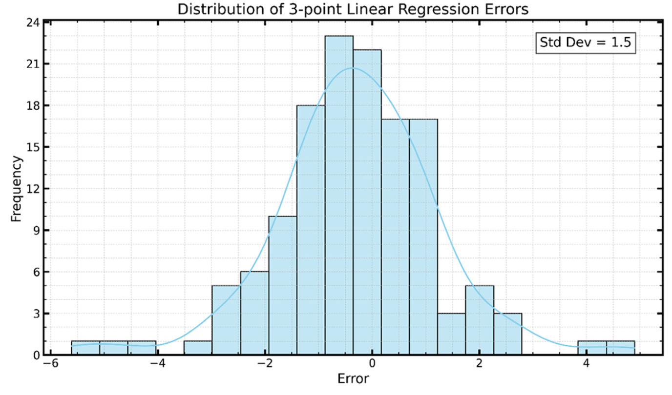
Distribution of the 3-point linear regression errors approximated as a normal distribution.
Using the prescribed procedure, transition probabilities may be computed for the 17 continue transitions leaving each state. Following are further details:
The decision horizon extends indefinitely into the future, with future rewards discounted by a factor
Utilities are computed using value iteration until convergence, when the maximum absolute change in state utility between successive iterations falls below
A self-loop is defined for “homogeneous” states, which are states containing identical elements such as (84,84,84), indicating no progression. Therefore, MDP is forced to recommend stopping at these terminal states.
The transition probabilities are normalized by their summation to ensure
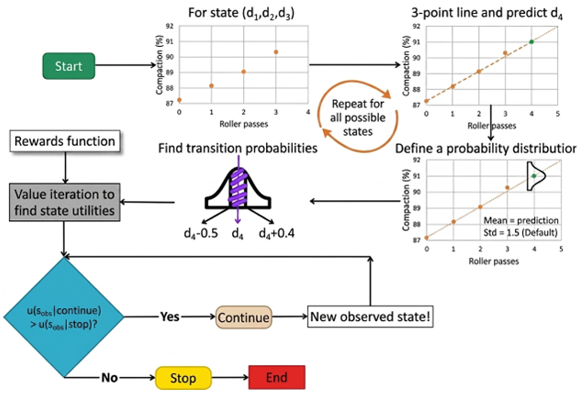
Flowchart for calculating transition probabilities and decision-making.
Rewards
Two different reward approaches for IDOT’s QCP and PFP programs were developed in this study. Both account for operational costs and pay factors by agencies, as detailed in the following subsections.
Operational Costs
Operational costs must be considered because contractors account for them when bidding for any pavement construction project. It is expected that MDP decisions will alter the construction time and, thus, the operational costs of the project (by recommending stopping or continuing compaction). The contractor usually considers the following:
Pavement construction costs are divided into three main categories: materials, operation, and materials transport.
Materials and transport costs are project dependent. They depend on tonnage and hauling distance, among other factors, but are less dependent on construction time.
The operational costs for a project include labor and equipment categories. These categories are dependent on construction time and may be altered. These costs include construction, traffic control, and testing activities. Traffic control and testing activities may be assumed a fixed cost of around $3,200/day for a typical project. Other costs can be estimated based on hourly rate ($/h) and working hours (h/day), as shown in Table 1.
Typical Labor and Equipment Costs Breakdown
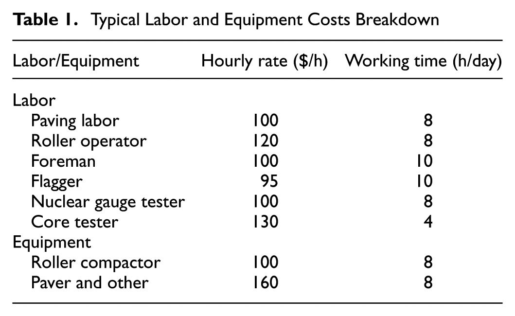
For a 4,500 ton project, the crew is typically composed of five paving laborers, two roller operators, one foreman, two flaggers, one nuclear gauge tester, and one core tester with two roller compactors and one paver. The compound cost of this crew, in addition to the fixed costs, is $16,200/day or $2,025/h. Using the previous observations about segment length, roller compactor speed, and number of passes per segment, it is estimated that the duration for one roller pass is 35 s (not considering breaks/delays). Accordingly, the $2,025/h operational cost translates to $20/roller pass. This cost is additive whenever the decision is to continue compaction. The GPR equipment cost was not included in this analysis because there are no commercial roller mounted-GPR systems on the market yet.
QCP Pay Factor
For QCP projects, IDOT specifies the pay factor based on the mix type: HMA versus stone-matrix asphalt (SMA), with a stricter acceptable density range for SMA [92, 98] than HMA [90, 98]. SMA is a special type of HMA characterized by higher asphalt binder content and a more stable stone-on-stone skeleton, which results in a relatively more expensive, but rut-resistant, mix ( 42 ).
As expected, agencies’ target densities are in the middle of the acceptable density range to avoid under- and over-compaction, as discussed in the introduction. Therefore, the highest pay factors are obtained for densities around 94% for HMA, and 94.5% for SMA, as shown by the red dashed lines in Figure 7. A pay factor of 105% indicates a bonus of 5% of contracted value, whereas a pay factor of 90% indicates a penalty of 10%.
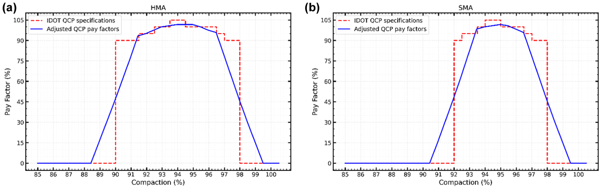
Original and adjusted Illinois Department of Transportation (IDOT) quality control for performance (QCP) pay factors for Markov decision process rewards for: (a) hot-mix asphalt (HMA) and (b) stone-matrix asphalt (SMA).
For the rewards function, it can mimic this stepped pay factor function. However, there is one caveat, which is the GPR error. It was reported that GPR prediction had an average error of
PFP Pay Factor
For PFP projects, IDOT specifies the pay factor based on the asphalt concrete mix type: IL-4.75, IL-9.5/IL-9.5FG, IL-19.0, and SMA mixes, with different and stricter density acceptance ranges than QCP: [92.5, 97.5], [91.5, 97.5], [92.2,97.5], and [93.0, 98], respectively). In addition, IDOT collects cores and assumes a t-distribution of the densities across the project. The pay factor is calculated based on the concept of percent within limits (PWL), as shown in Equation 5. PWL is calculated as the area under the PDF of the fitted t-distribution within the specified limits, allowing for project variability consideration in the pay:

GPR data from three projects in Illinois, near Gilman, Kankakee, and South Holland, were analyzed to quantify the spatial variability in density prediction within each roller pass. Although additional projects should be considered in the future, the analyzed projects involved two different contractors, three different roller operators, and asphalt mixtures with different aggregate types and gradations, P b and G mm values, and recycled material contents. In total, 206 different passes were analyzed and fitted to t-distributions. Examples of these t-distributions from each project are shown in Figure 8. Notably, t-distributions fit the data well. An average SD of 1.6 was calculated for the 206 passes. This SD differs from one project to another, one contractor to another, and one pass to another. Generally, later passes showed lower SD than initial ones.
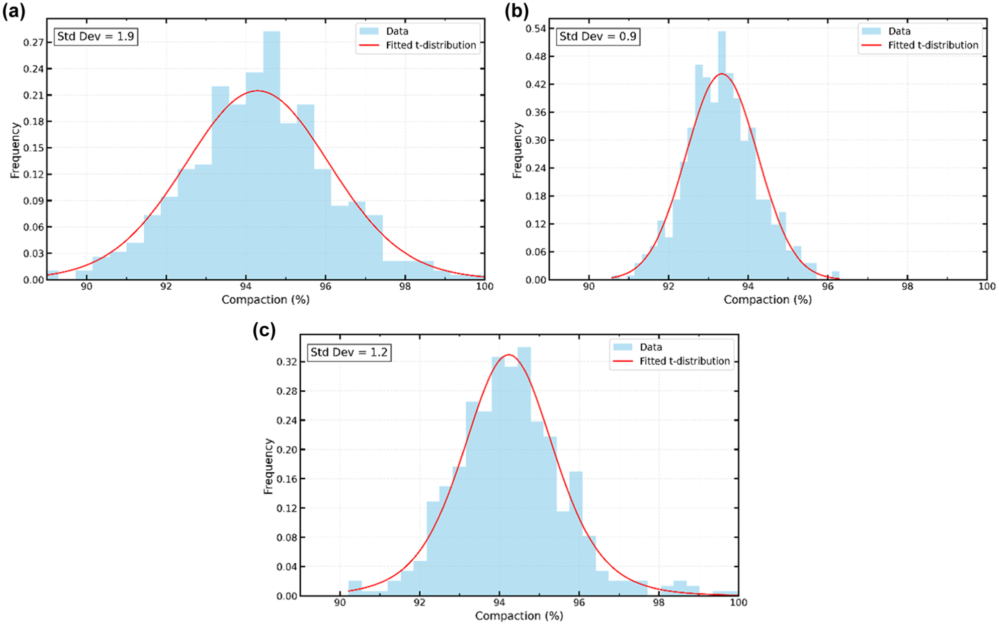
Example t-distributions from: (a) third pass on a segment near Gilman, (b) tenth pass on a segment near Kankakee, and (c) first pass on a segment near South Holland.
This average SD is considered high, because, when coupled with a mean value in the middle of the acceptable range, the pay factor is 100% (best case scenario results in no bonus). On the contrary, some contractors get bonuses because of sporadic checks, a lower achieved variability, or both (required SD = 0.75 to achieve 5% bonus at midrange density). Therefore, an SD of 1.6 is chosen to account for both GPR error and spatial variability. Consequently, when the state density is 94%, a t-distribution of mean = 94 and SD = 1.6 (default) is defined for the pass to calculate PWL, pay factor, and expected rewards. Figure 9 shows the original (dashed red) and adjusted (continuous blue) pay factors for all mix types. This necessarily means that the calculated rewards only approximate—and do not exactly represent—the contractors’ pay, since the results depend on the contractor’s compaction variability and locations of core checks.
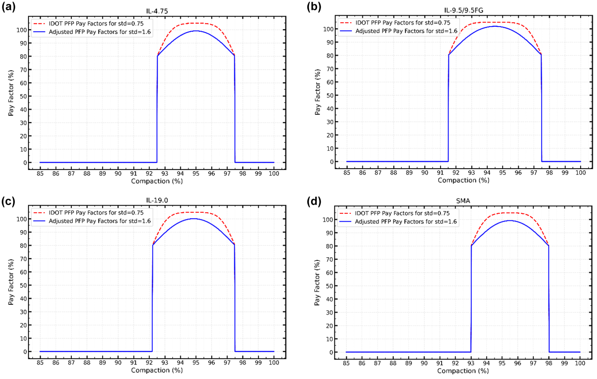
Original and adjusted Illinois Department of Transportation (IDOT) pay for performance (PFP) pay factors for Markov decision process rewards for: (a) IL-4.75, (b) IL-9.5 and IL-9.5FG, (c) IL-19.0, and (d) stone-matrix asphalt (SMA).Note: IL-4.75, IL-9.5, IL-9.5FG, and IL-19.0 are asphalt concrete mixes with different aggregate gradations defined by IDOT.
The following are further details for the rewards:
The pay factor for density is only 40% of the CPF in Illinois, as explained in the introduction.
The pay factor must be multiplied by sub-lane value to calculate the expected reward per sub-lane. This is because density progression curves are presented per sub-lane. A sub-lane value may be estimated based on the project value, an assumed crew productivity, and other rolling pattern-related assumptions mentioned earlier.
Defined rewards are a function of the state and the action. If the action is to continue, only immediate operational costs are considered. On the other hand, when the action is to stop, the pay factor based on the realized final density is included. This avoids repeatedly counting the pay factor in rewards.
For example, for a project with 4,500 tons (5.9 mi [9.5 km] of 2 in. [5 cm] lift thickness and 145 lb/ft3 [2,323 kg/m3] HMA density), and four construction days (around 1,000 tons/day), using the previous assumption of 220 ft (67 m)-long segments, there will be 141 segments in total, paving about 35 segments/day. For this project, with a total value of $650,000, the value of a sub-lane (assuming three sub-lanes/segment) may be calculated as follows:
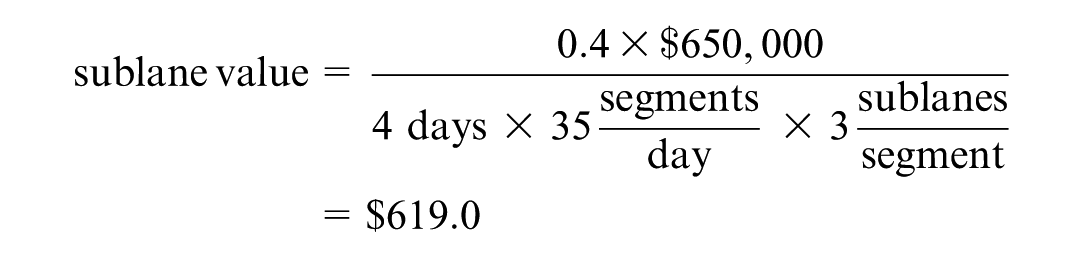
The rewards are calculated by multiplying the pay factor with the estimated sub-lane value. In the case of unacceptable density, the rewards are calculated as 0, −0.5 x sub-lane value, and −1 x sub-lane value, for the cases of rejection, removal, and reconstruction penalties, respectively.
MDP Demonstration
To demonstrate MDP behavior and impact, data from an HMA project were used to compare the rolling pattern of an experienced roller operator to MDP decisions. The project is a gas station parking lot near Bourbonnais, IL, contracted by Gallagher Asphalt Co. The project consisted of a 5 in. (12.7 cm) binder course (IL-19.0) and 3 in (7.6 cm) surface course (IL-9.5), as shown in Figure 10a. The total tonnage was about 2,800 tons which means that it is under the QCP program. The project was visited on October 30, 2023, and GPR data were collected on the surface course using roller-mounted GPR, as shown in Figure 10b. HMA design was provided by the contractor and used to predict the HMA density progression curves using the ALL model. The GPR was mounted on a tandem finishing roller with 78 in. (2 m) drum width.
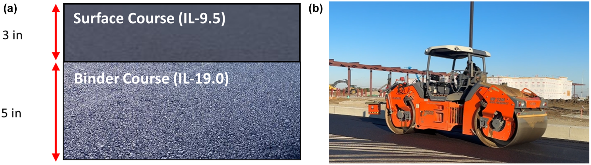
Parking lot project: (a) layer configuration and (b) roller-mounted ground-penetrating radar setup.
Data from five lanes (15 segments = 45 sub-lanes) were analyzed in this study, and conclusions may be extended to the whole project. Each lane was about 465 ft (141.7 m) long. A test pad was constructed at the beginning of the project and a nuclear gauge was used during compaction to monitor density. As inputs, a project value of $650,000, and four construction days were used. The crew consisted of five paving labor, three roller operators, one foreman, zero flaggers, one nuclear gauge tester, and one core tester, in addition to one paver and three roller compactors for equipment. In the case of unacceptable density, rejection was applied (0 rewards). The same project data was analyzed under the PFP program (hypothetical scenario), with the assumptions of triple the tonnage (>8,000), construction days, and project value. A reconstruction penalty is applied in the case of unacceptable density to verify MDP behavior under stricter and higher risk conditions. Based on these inputs, a cost of $19.5/pass and a value of $619.0/sub-lane were calculated.
During the field visit, the roller operator followed their normal rolling pattern without receiving any MDP guidance or GPR-based predictions. After data collection and processing, the predicted density progression curves were provided to MDP, which used the first three points and then one additional point at a time to make sequential decisions. These MDP decisions were then compared with the operator’s actual decisions evidenced by the full density progression curves recorded in the field, to assess the impact of MDP on rolling pattern optimization.
Analysis and Results
QCP Scenario (Actual)
Figure 11 presents MDP versus roller operator behavior in a chosen number of passes and the resulting final density under the QCP program. For consistency in comparison, the density progression curve predicted by GPR following the roller operator’s actual rolling pattern is treated as the reference (i.e., “realized” outcome). The MDP framework does not generate independent field measurements; rather, it uses a transition model to predict future density values and determine whether to continue compaction or stop, based on maximizing expected rewards (i.e., agency pay factors minus operational costs). Once MDP recommends stopping compaction, the corresponding realized density from the GPR density progression curve at that pass is used for comparison.
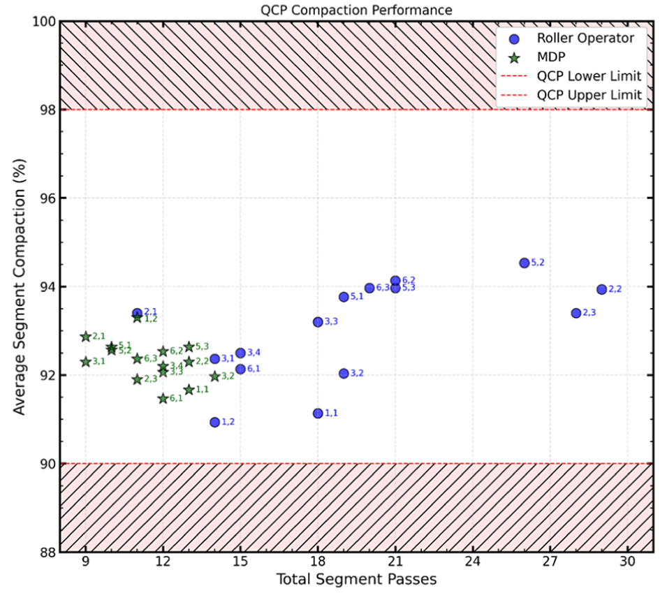
Markov decision process (MDP) compaction performance under Illinois’ quality control for performance (QCP) specifications.
Generally, MDP decisions tend to reduce the number of passes, while still achieving acceptable density based on QCP specifications. In some cases, such as lane 3 segment 2 (point labeled 3,2), early stopping resulted in a similar average final density, avoiding extra operational costs. Figure 12 shows an example behavior for the left sub-lane of this segment, where the predicted next densities are indicated by the black boxes with their corresponding probabilities. Note that the “observed” densities by MDP are the integer version of the GPR predictions because of state definition. In other cases, early stopping resulted in even higher (point [1,1]) and sometimes lower (point [3,3]) density. However, it was preferred because of negligible expected future incentives. Overall, using MDP resulted in 172 total passes instead of 288, which is about 40.3% reduction in construction time.
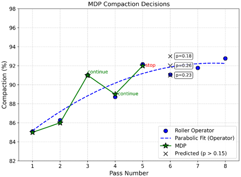
Markov decision process (MDP) behavior for lane 3, segment 2, left sub-lane.
If MDP recommends more passes than were performed by the roller operator, then no realized field density is available for the comparison. In that case, the most probable MDP-predicted densities from the transition model are used as the final densities corresponding to the additional passes suggested. This case was only observed for lane 1, segment 2, left sub-lane, where the final density by the roller operator was 90.7%, which is close to the lower acceptance threshold of 90%, and, therefore, MDP recommended an additional pass. Table 2 presents the results for all the analyzed sub-lanes under QCP scenario.
Markov Decision Process (MDP) Analysis Results for Illinois’ Quality Control for Performance (QCP) Program
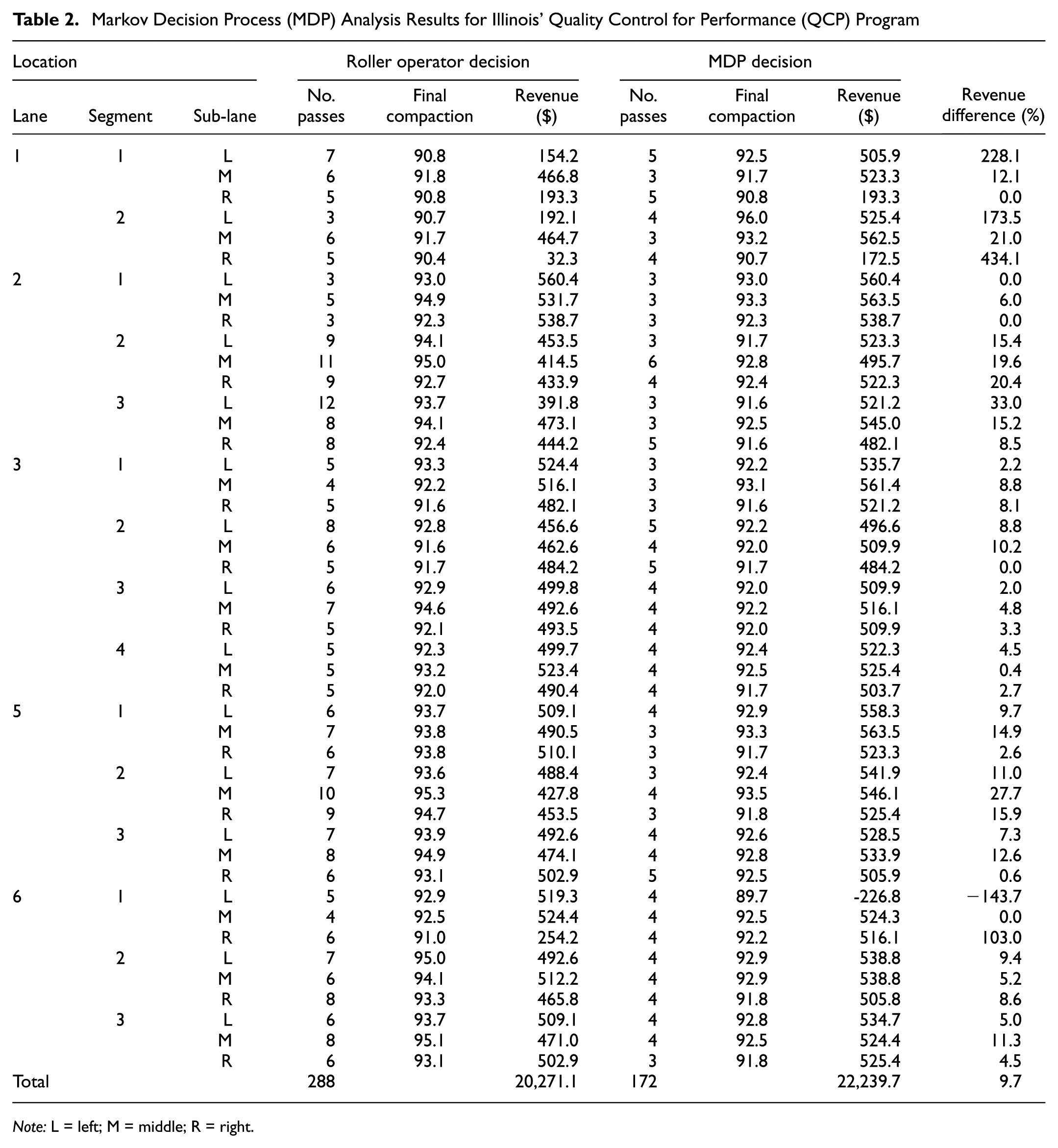
Note: L = left; M = middle; R = right.
Figure 13 presents the associated impact on the revenue. Revenue is computed by combining the expected agency pay factors (based on the realized density per segment) with the corresponding operational costs (based on the selected number of roller passes
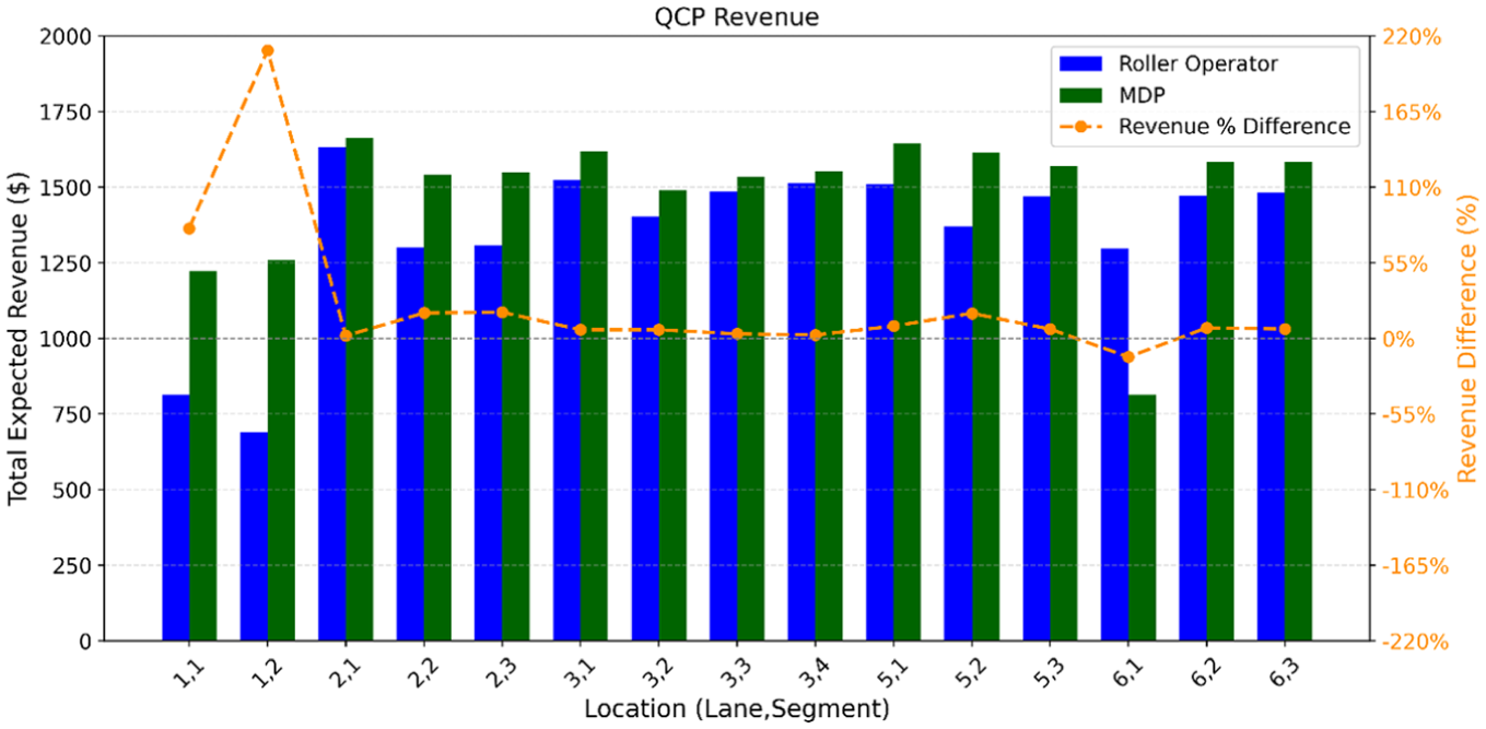
Markov decision process (MDP) impact on revenue under Illinois’ quality control for performance (QCP) specifications averaged over sub-lanes.
The reduced-revenue case occurred in lane 6, segment 1, left sub-lane and is shown in Figure 14. Here, the transition model assigned relatively high probabilities to either a similar next density (26%) or a lower next density (23%), and therefore recommended stopping to minimize potential penalties. In reality, however, the density increased. This mismatch may be attributed to limitations in the transition model, the use of integer-valued states, and/or the accuracy of the GPR processing algorithms. For instance, the actual density at the critical pass was 89.7%, which is unacceptable, while the GPR-based state used in MDP was rounded to 90%, which is acceptable.
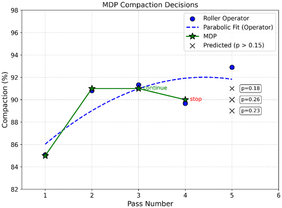
Markov decision process (MDP) behavior for lane 6, segment 1, left sub-lane.
A further observation for this case is the wide spread of roller paths within the sub-lane, as indicated by the GPS traces in Figure 15. Differences in pass location and pass length can affect the density progression curve because of the spatial variability of HMA density. In particular, pass 4 was located farther north than the adjacent passes and covered a greater length than passes 3 and 5. These findings suggest that pass alignment characteristics should be incorporated into future decision-making, for example through thresholds on valid pass length and allowable distance from the sub-lane centerline.
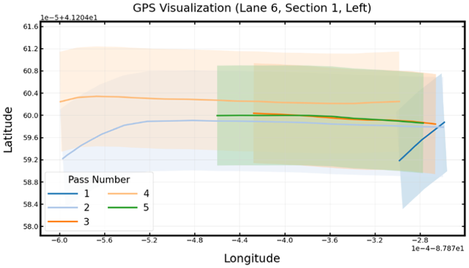
Global Positioning System (GPS) paths for roller passes for lane 6, segment 1, left sub-lane.
PFP Scenario (Hypothetical)
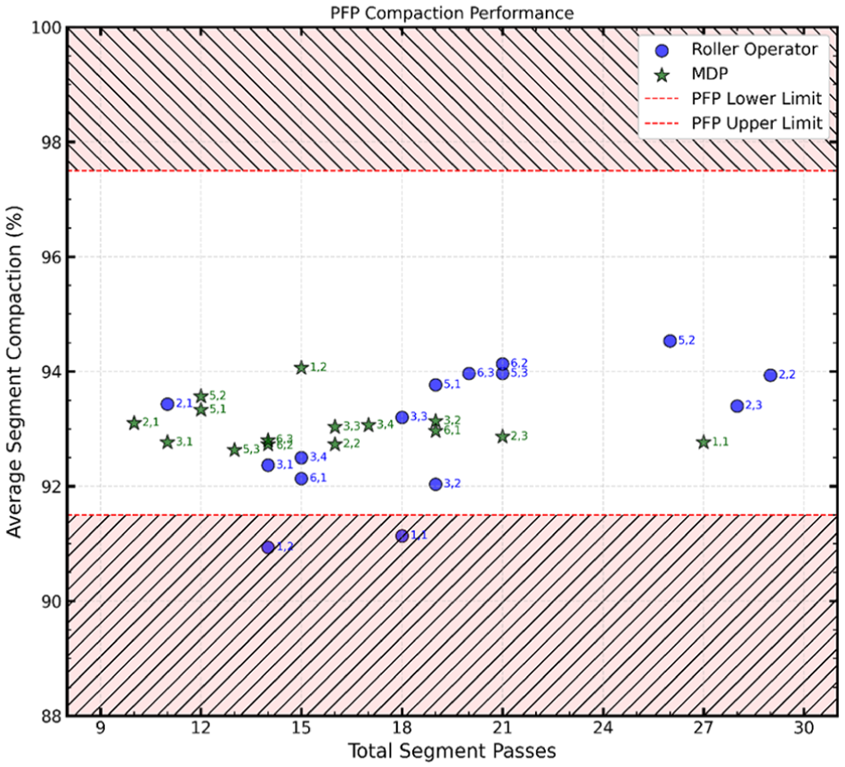
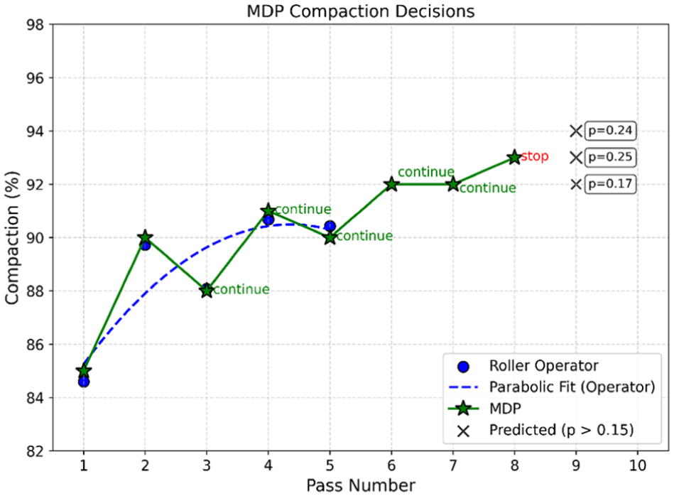
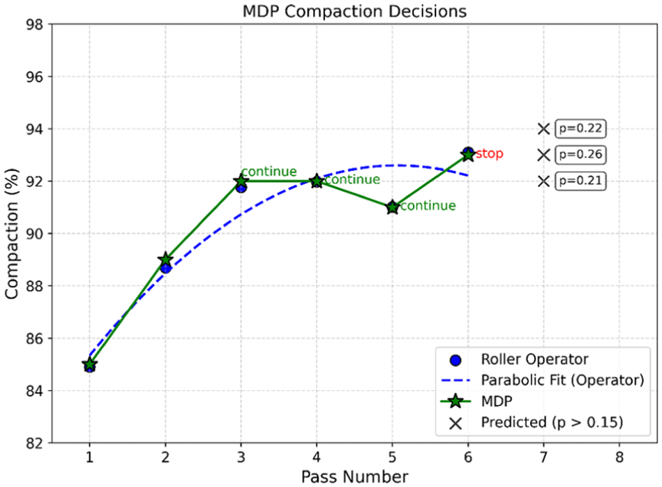
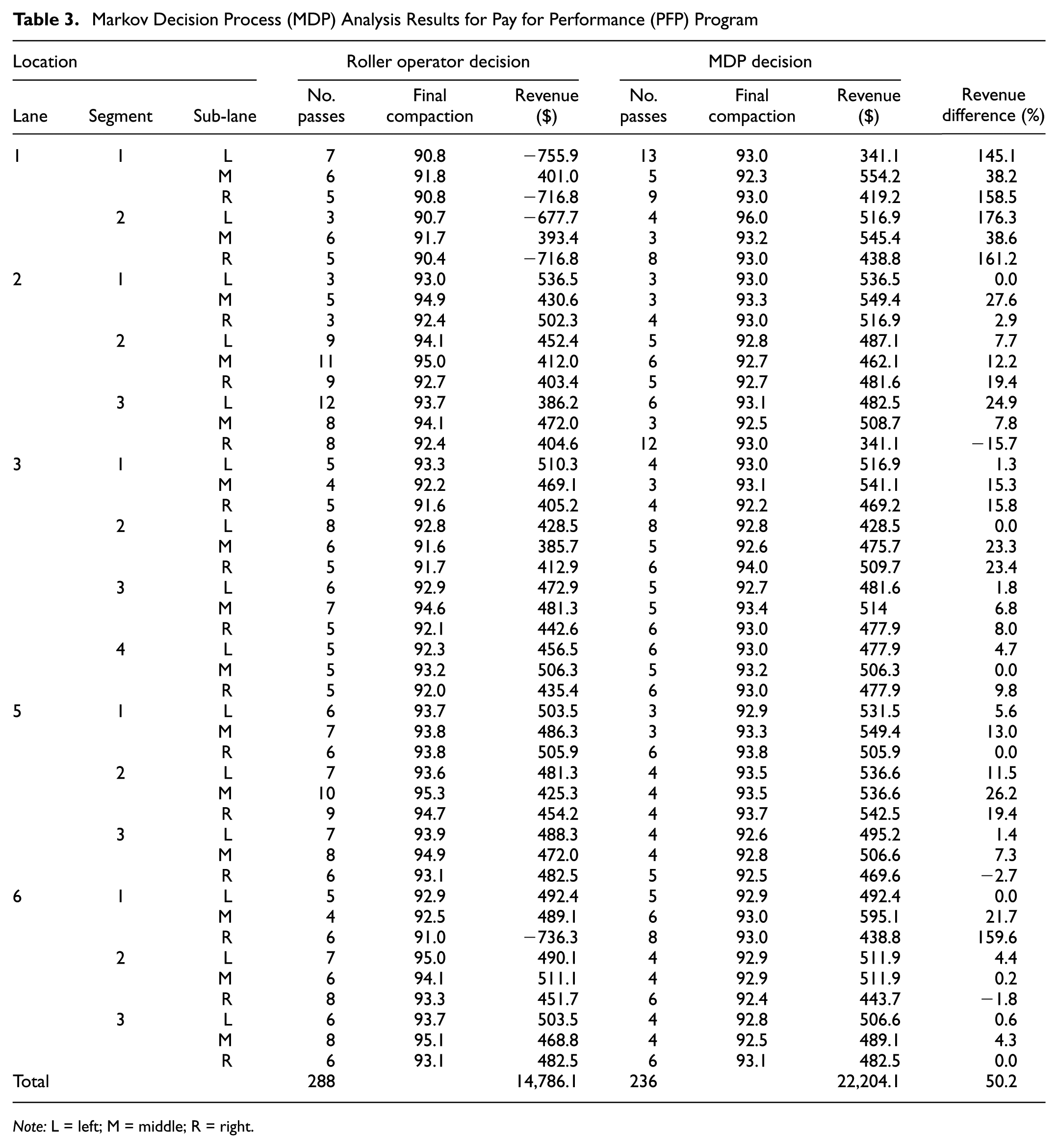
For the PFP hypothetical scenario, Figure 16 compares the compaction behavior of MDP with the roller operator. In most cases, MDP recommended fewer passes, but in many other cases, MDP recommended more passes. One notable example is segment (1,1), where MDP recommended many extra passes, incurring additional operational costs, to avoid the high reconstruction penalty. Similarly, for segment (1,2), MDP recommended additional passes to recover the segment, as shown in Figure 17. For lane 6, segment 3, right sub-lane, MDP and the roller operator reached the same decision, as illustrated in Figure 18. Table 3 summarizes the results for all analyzed sub-lanes under the PFP scenario.
Markov decision process (MDP) compaction performance under pay for performance (PFP) specifications.
Markov decision process (MDP) behavior for lane 1, segment 2, right sub-lane.
Markov decision process (MDP) behavior for lane 6, segment 3, right sub-lane.
Markov Decision Process (MDP) Analysis Results for Pay for Performance (PFP) Program
Note: L = left; M = middle; R = right.
For the PFP scenario, MDP behavior was more conservative to adhere with the stricter density specifications and avoid the high penalty in the case of unacceptable density (reconstruction). Accordingly, the total number of passes only reduced from 288 to 236, which is about 18.1% reduction. For the revenue, as shown in Table 3, 6 out of 45 cases show no difference in revenue meaning that the MDP decisions agreed with the roller operator; 36 out of 45 cases show increased revenue; and 3 out of 45 cases show decreased revenue. Using MDP in the PFP scenario increased the total revenue by 50.2%, which is equivalent to 10.7% of the project value (assuming similar behavior for the remaining segments and construction days). This pronounced revenue increase is because this is a hypothetical scenario where the actual roller operators’ decisions were made under the QCP program with a wider range of acceptable densities and lower penalty (Figure 19).
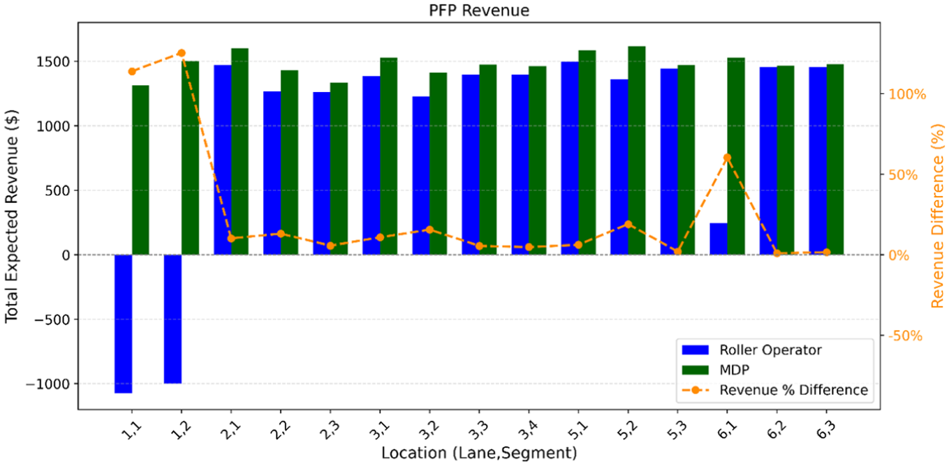
Markov decision process (MDP) impact on revenue under pay for performance (PFP) specifications averaged over sub-lanes.
The case of lane 2, segment 3, right sub-lane is shown in Figure 20 as an example of reduced revenue. This outcome is attributed to the use of integer-valued states in the MDP formulation, whereas the agency pay factors are defined as continuous functions of density. At pass 8, the realized density was 92.4%, corresponding to a pay factor of 0.91. However, within the MDP framework, this value was represented by the integer state of 92%, which corresponds to a lower pay factor of 0.86. Consequently, MDP recommended additional passes until a density of 93% was reached; however, the actual increase in density does not justify the additional operational costs. In future work, using decimal-place-level state definitions may improve MDP performance. A hybrid approach could also be considered, where finer state resolution is applied only near agency-specified density thresholds to improve decision accuracy while limiting the dimensionality burden.
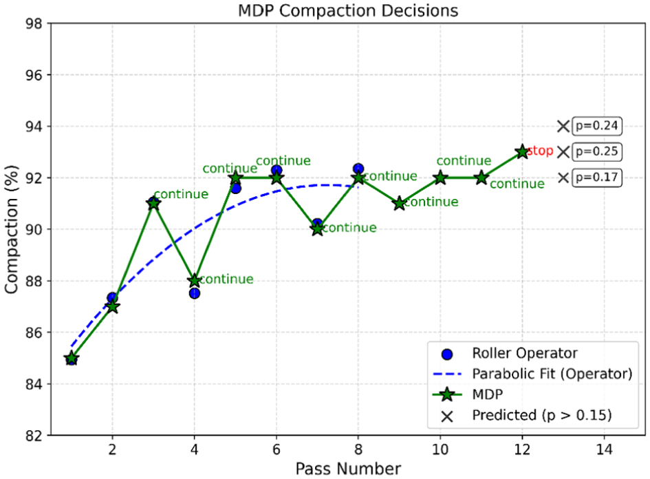
Markov decision process (MDP) behavior for lane 2, segment 3, right sub-lane.
Notably, saving 40.3% and 18.1% in construction time (for QCP and PFP scenarios) may result in reducing the number of construction days, which entails savings in mobilization, material transport, and other costs that were assumed fixed. Accordingly, the savings might be higher than reported.
Conclusions and Recommendations
HMA contractors can optimize their rolling pattern by using real-time GPR density monitoring data to make informed decisions “on the go.” An MDP is formulated in this study to optimize the rolling pattern. The optimization considers the project’s operational costs and expected pay factors by agencies. The following are some conclusions:
The introduced MDP framework can model the rolling pattern while accounting for uncertainty in the GPR predictions, spatial variability, and uncertainty in the density progression.
Compared with an experienced roller operator, the MDP approach could save compaction time through guiding operators to reach target density, maximizing cost savings.
The developed MDP was applied to data from an actual project under QCP and PFP (hypothetical) acceptance scenarios. For the QCP scenario, MDP resulted in saving 40.3% of the compaction time and increasing revenue by 9.7%. For the PFP scenario, MDP resulted in saving 18.1% of the compaction time and increasing revenue by 50.2%. The revenue increase translates to about 2.8% and 10.7% of the project value for QCP and PFP scenarios, respectively.
The formulated MDP showed a generalizable beneficial behavior under two different quality acceptance programs of different risks and specifications.
The additional benefits of using MDP include saving energy, reducing construction zone delays, enhancing workers’ safety, and ensuring achieving HMA density that increases pavement service life and reduces costly maintenance activities for agencies.
Work is underway to reduce GPR prediction error, improve transition models, and demonstrate MDP application on additional HMA field projects. Future work will also explore more advanced formulations, such as partially observable MDPs, that incorporate additional operational parameters (e.g., roller speed) to improve state estimation and decision-making.
Footnotes
Acknowledgements
The authors greatly appreciate the support of Gallagher Asphalt Co., especially Brian Gallagher for coordinating field visits and communicating project data, Jeffery Kolmodin for the project breakdown costs, and Steve Rubio for collaborating during field measurements. The authors would like to acknowledge the help of Yanfeng Ouyang, Yihan Chen, Javier Garcia-Mainieri, Lara Diab, Egemen Okte, Akash Bajaj, and ICT research engineers Greg Renshaw, Mohsen Motlagh, and Uthman Mohammad Ali. The authors are representatives of the Illinois Center for Transportation (ICT).
Author Contributions
The authors confirm contribution to the paper as follows: study conception and design: I. Al-Qadi, L Abufares; data collection: L. Abufares, I. Al-Qadi; analysis and interpretation of results: L. Abufares, I. Al-Qadi, M. Hasegawa-Johnson; draft manuscript preparation: L. Abufares, I. Al-Qadi, M. Hasegawa-Johnson. All authors reviewed the results and approved the final version of the manuscript.
Declaration of Conflicting Interests
The authors declared no potential conflicts of interest with respect to the research, authorship, and/or publication of this article.
Funding
The authors received no financial support for the research, authorship, and/or publication of this article.

The contents of this paper reflect the views of the authors, who are responsible for the facts and the accuracy of the data presented. The contents do not necessarily reflect the official view or policies of ICT. This paper does not constitute a standard, specifications, or regulations.