Cortical Bony Thickening of the Lateral Intercondylar Wall: The Functional Attachment of the Anterior Cruciate Ligament

Abstract

Background:

The anatomy of the anterior cruciate ligament (ACL) has become the subject of much debate. There has been extensive study into attachment points of the native ligament, especially regarding the femoral attachment. Some of these studies have suggested that fibers in the ACL are of differing functional importance. Fibers with higher functional importance would be expected to exert larger mechanical stress on the bone. According to Wolff’s law, cortical thickening would be expected in these areas.

Purpose:

To examine cortical thickening in the region of the ACL footprint (ie, the functional footprint of the ACL).

Study Design:

Descriptive laboratory study.

Methods:

Using micro–computed tomography with resolutions ranging from 71 to 91 μm, the cortical thickness of the lateral wall of the intercondylar notch in 17 cadaveric knees was examined, along with surface topography. After image processing, the relationship between the cortical thickening and surface topology was visually compared.

Results:

A pattern of cortical thickening consistent with the functional footprint of the ACL was found. On average, this area was 3 times thicker than the surrounding bone and significantly thicker than the remaining lateral wall (P < .0001). This thickening was roughly elliptical in shape (with a mean centroid at 23.5 h:31 t on a Bernard and Hertel grid) and had areas higher on the wall where greater thickness was present. The relationship to previously reported osseous landmarks was variable, although the patterns were broadly consistent with those reported in previous studies describing direct and indirect fibers of the ACL.

Conclusion:

The findings of this study are consistent with those of recent studies describing fibers in the ACL of differing functional importance. The area in which the thickening was found has been defined and is likely to represent the functional footprint of the ACL.

Clinical Relevance:

This information is of value to surgeons when determining the optimal place to position the femoral attachment site of the reconstructed ACL.

Keywords

anterior cruciate ligament attachment site micro-CT measurement ACL anatomy

The anatomy of the anterior cruciate ligament (ACL) has become the subject of much debate. Concerns about the optimal position for ACL reconstruction have sparked extensive study into the shape, orientation, and attachment points of the native ligament, especially regarding the femoral attachment.^{7,8,10,15,24,28,32}

The femoral soft tissue attachment of the ACL is not a circle but an ellipse, as recently highlighted by Fu and Jordan,⁹ who noted along with others that the majority of the fibers lie posterior and proximal to the lateral intercondylar ridge. More recently, Iwahashi et al¹⁴ demonstrated a direct and indirect insertion of the ACL on the femoral condyle, with the direct insertion of the ligament acting as “a key link between the ligament and bone to transmit mechanical load to the joint.” The “ribbon” concept of the ACL has also been described recently,²⁴ emphasizing the fact that not all of the fibers of the ACL are equally functional.

While numerous surface landmarks have been identified to help guide the surgeon in placing a graft, the intraoperative identification of these landmarks is not always straightforward.³² In previous work at our institution,^2,20 we used micro–computed tomography (micro-CT) to a resolution of ≈60 μm to assess bony landmarks described by Fu and Karlsson,⁹ demonstrating that the osseous landmarks were variable.^2,20 However, while examining the surfaces of the femoral condyles, we noted a thickening of the cortical bone in the region of the ACL attachment that warranted further investigation.

It is well recognized that bone is highly adaptive to the mechanical stresses placed on it, originally described as Wolff’s law.³⁰ Bone is thicker in areas of high stress, and therefore the pattern of cortical thickness is able to define the areas of high stress in the lateral intercondylar wall, allowing us to define a functional footprint for the ligament. This will also potentially identify the most mechanically active part of the footprint, as opposed to its entire soft tissue attachment.^11,29 The aim of this study is therefore to examine the functional footprint of the ACL using micro-CT with a view to defining its anatomy and location on the lateral wall of the intercondylar notch.

Methods

Samples and Imaging Technique

Seventeen cadaveric knees donated by 13 individuals were included, of which 7 were included from a previous study.²⁰ Cadavers from 4 females and 9 males (4 left/right matched pairs) aged between 63 and 82 years were donated for this study. Knees were sourced after approval by our hospital’s research and development department but did not require further ethics approval. All specimens were micro-CT scanned using a Nikon XTH320LC micro-CT scanner with parameters 255 kV, 18 W, 1-second exposure, with a 1-mm copper filter resulting in resolutions ranging from 71 to 91 μm. All knees underwent arthroscopic evaluation by a highly experienced ACL surgeon using arthroscopic instruments. In the first 10 knees, the micro-CT scans were performed before the arthroscopy; in the subsequent 7 knees that were included from the previous study, the scans were performed after the arthroscopy.

Cortical Thickness Mapping

To visually represent cortical bony thickness on both the lateral intercondylar wall and medial intercondylar wall, ImageJ open source image processing software (National Institutes of Health) was used. ImageJ is frequently used in biomedical research²³ and contains open source plugins that implement published algorithms for image processing. In this study, the plugin BoneJ was used to “define the thickness at a point as the diameter of the greatest sphere that fits within the structure that contains the point.”^5,6 This algorithm allows the thickness of a 3-dimensional (3D) shape to be colored at every point depending on the structure’s thickness at that point.¹³ The cortical bone thickness of the distal 10 cm of the femur was mapped in 3 dimensions. To ensure that the patterns observed were not structural features of the intercondylar notch and were representative of ligament attachments, both the medial and lateral walls were examined. Sagittal views of the lateral and medial walls (with the femur cut in its midsagittal plane) were extracted with the femoral shaft aligned horizontal to and the plane of view directly perpendicular to the surface of the wall. Furthermore, as part of the cortical thickening algorithm, BoneJ provides the ratio of bone volume to trabecular volume (BV/TV), typically used as a measure of bone density for each femur.

While these maps provide the primary data on cortical thickness, it was decided that some form of measurement was required to map the anatomy in a way that could be related to other work in the literature. Therefore, to describe these regions in terms of relative location, width, and length, an appropriate shape had to be fitted to the visually thicker cortical region. An ellipse was determined as the simplest and most appropriate fit to model the observed shapes, allowing width, length, and orientation to be defined. This was performed by the author trained in image processing techniques (D.N.) and allowed for a best-fit approximation typically required when modeling complex shapes. The Bernard and Hertel¹ grid method was used to define the coordinates of the centroid of the ellipse. This technique projects a grid onto the lateral plane of the lateral intercondylar wall, with distance t being the sagittal diameter of the lateral condyle measured along the Blumensaat line and distance h being the maximal height of the notch. In addition, measures of the width and height of the area were taken as well as the angle of the ellipse to the Blumensaat line (θ) (see Figure 5A).²⁷ The thickness of the area was defined as the mean (±SD) thickness within the fitted ellipse and was compared with the thickness of the remainder of the lateral wall. A nondirectional paired-samples t test was conducted across all samples to compare the thickness within the ellipse against that of the remaining part of the lateral wall.

These ellipses could then be combined to produce a diagram depicting where thickening occurred in our complete sample. By scaling, transforming, and aligning all sagittal views of the lateral wall, overlaying of all regions of thickness was possible. The ellipses approximating the cortical thickened region were colored red at 90% transparency to allow the reader to appreciate the typical region of thickness, including its full variation within this sample. The same process was followed to allow identification of areas within the ellipse that were even thicker, approximating the very thick regions as a 90% transparent yellow ellipse overlaid onto the typical region of thickness.

Surface Topology

In an attempt to objectively highlight any osseous landmarks present on the lateral wall, high-resolution relief maps of the surface topology were created using a previously published process.²⁰ These topological maps color the surface features based on height above a baseline surface, thereby revealing any landmarks present. Just as with the identification of osseous landmarks, interpretation of these relief maps can require experience; therefore, for the readers’ guidance, a further process was performed in which the ridge was defined as an ellipse (or a line at which a single-step cutoff was identified) by one of the authors (D.N.), who was trained in image analysis techniques.

Results

Seventeen cadavers were used for this study and were examined arthroscopically after or before (postoperative femurs only) micro-CT scanning. During this, femurs 1 and 8 were noted to have advanced osteoarthritis, with all other femurs having no other anatomic abnormalities with regard to either the lateral intercondylar wall or ACL bundles. The mean BV/TV for all femurs was 20%, with only femur 1 (16%) falling below 1 SD (±3.5%) of the mean. Analyzing the complex interactions between BV/TV, age, and osteoporosis was outside the remit of this study; however, it is noted that the mean BV/TVs here were within the range of nonosteoporotic reported values (19%-26%), particularly when accounting for the age of our samples.^4,12,16,19

Figure 1 provides a visual example of the micro-CT data before and after the thickness mapping process. The models have then been sectioned to allow the reader to appreciate the context of Figures 2 and 3. Figure 2 gives the cortical thickness maps of the lateral femoral condyle for each sample. It is apparent from Figures 1 and 2 that the roof of the notch showed substantial thickening, as expected, due to the structural stress-bearing nature of that region. To demonstrate that the thickening was not responsible for the thickening seen on the lateral wall, it was decided to include a figure showing the medial wall as well. Figure 3 gives the equivalent maps for the medial femoral condyle and has been included to visually demonstrate that the cortical thickening on both walls was not symmetrical due to the macro bony structure of the femur and, consequently, not simply a continuation of thickening originating from the roof of the notch. This therefore supports the hypothesis that the pattern is indeed from the function of the ligament attachment. A future study analyzing the medial wall is planned. The areas of cortical thickness can be seen on both walls, but those areas were in different locations on the medial and lateral walls, with the area of thickening much more anterior on the medial wall compared with the area of thickening on the lateral wall, consistent with the known attachments of the posterior and anterior cruciate ligaments, respectively.

Figure 1.

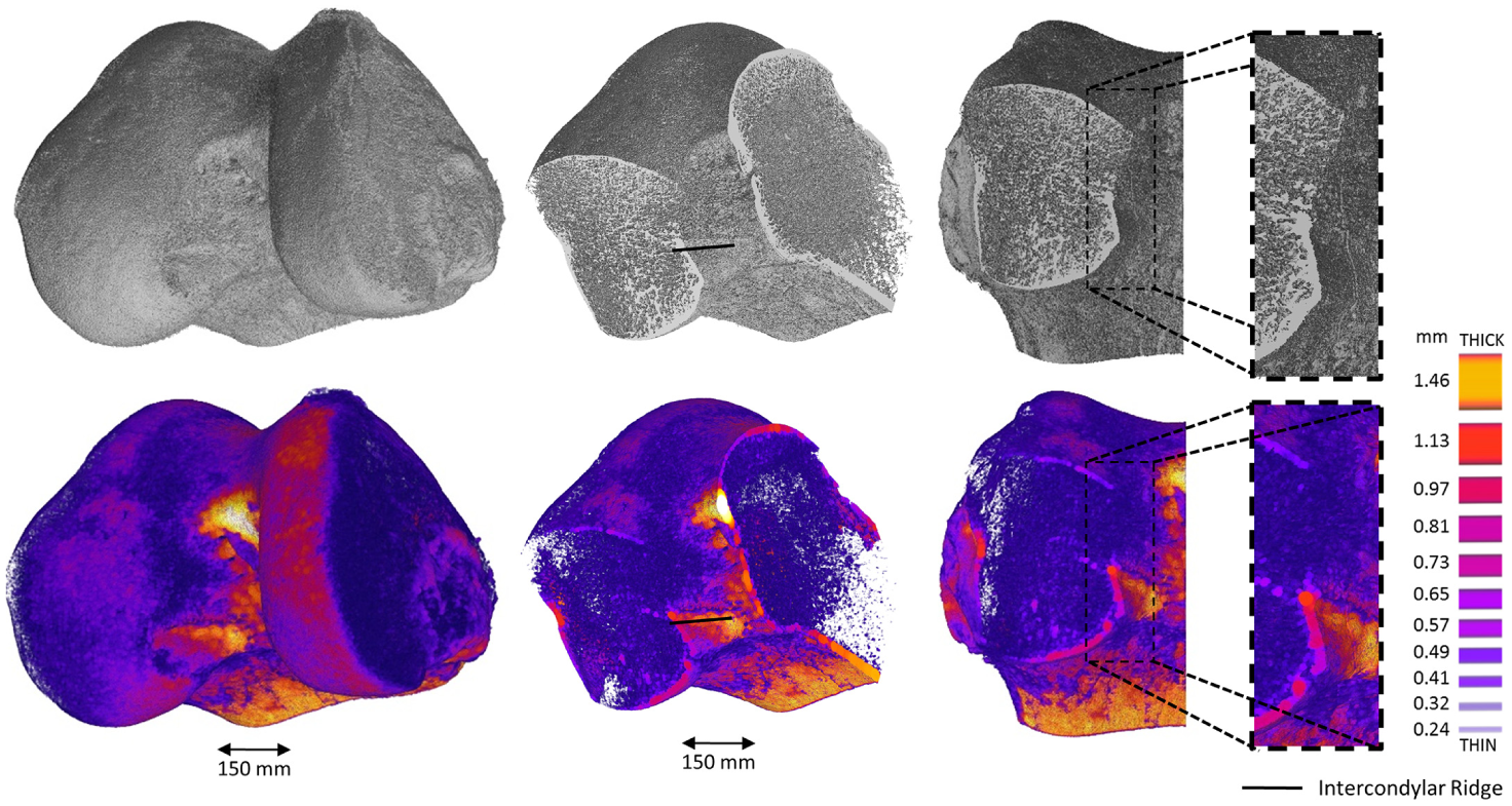
Micro–computed tomography (top) and cortical thickening maps (bottom) of the femoral head digitally sectioned perpendicular to, and 50% across, the lateral wall, resulting in a frontal-plane view of the lateral wall.

Figure 2.

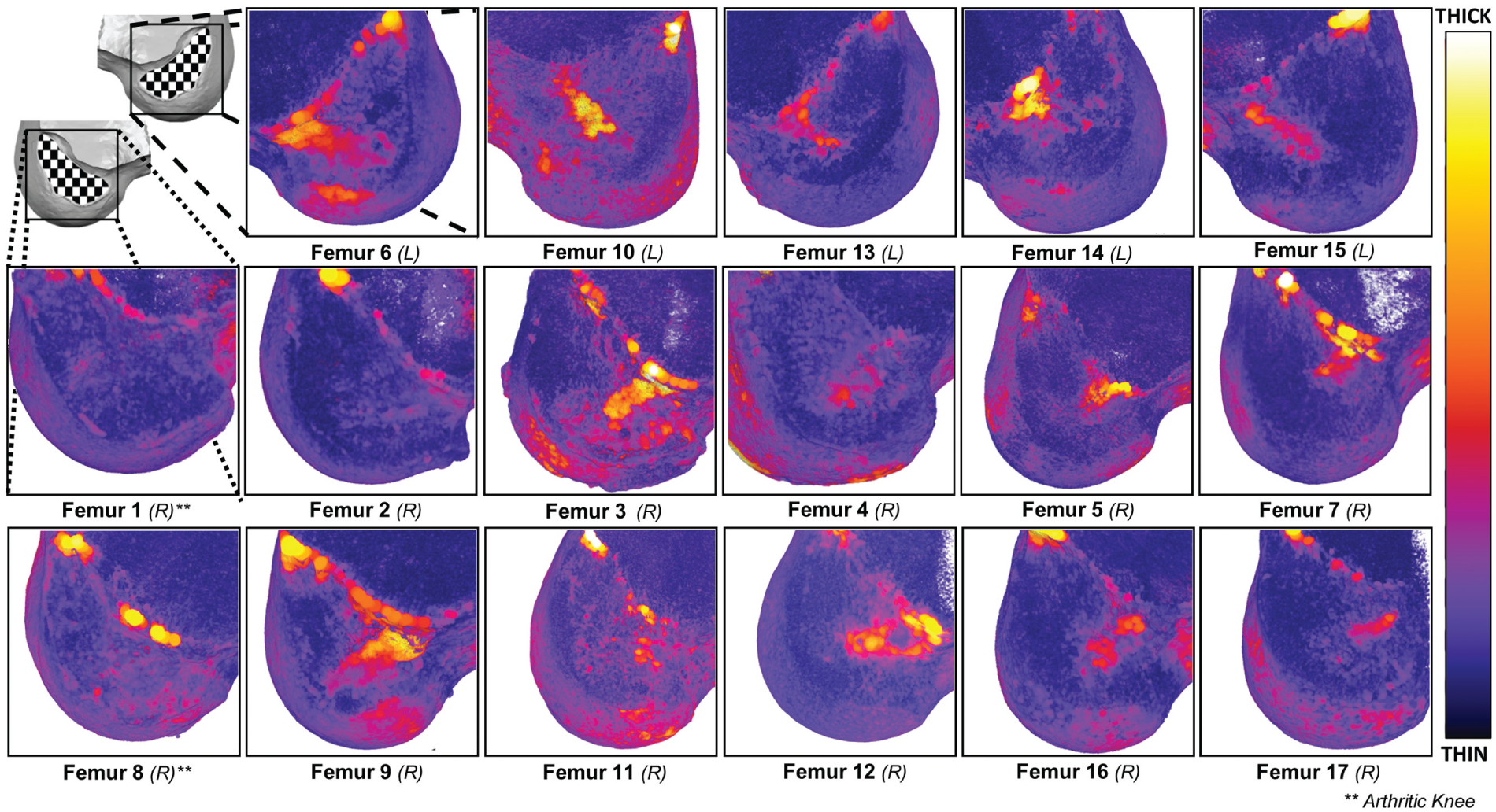
Cortical bone thickness maps with color scale of the lateral intercondylar wall for femurs in this study, with asterisks indicating whether femurs were arthritic.

Figure 3.

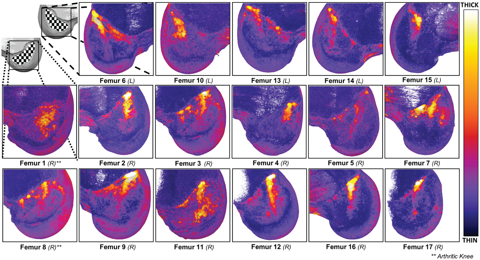
Cortical bone thickness maps with color scale of the medial intercondylar wall for femurs in this study, with asterisks indicating whether femurs were arthritic.

An ellipse could be fitted to a thicker area of the cortex in 15 of the 17 samples. In femurs 1 and 8, no area could be identified, although both of these cases were noted to have advanced degrees of osteoarthritis upon arthroscopic examination, as discussed above. Table 1 gives the details of the size, position, orientation, and location of the centroid of the fitted ellipses that were used to describe the areas of cortical thickening. The mean centroid was at 31% ± 3.4% depth and 23% ± 5.7% height from the proximal-anterior corner of the grid. The thickness of the identified areas is documented in Figure 4, demonstrating that the thicker regions were typically around 3 times thicker than the surrounding cortex of the intercondylar notch. A paired-samples t test to compare the lateral wall thickness (mean ± SD, 0.32 ± 0.06 mm) with the ellipse thickness (0.94 ± 0.15 mm) across the 16 femurs gave t(15) = 15.2, P < .0001, demonstrating a highly statistically significant difference in thickness. The absolute cortical thickness found in this study for the ACL footprint and remaining lateral wall is comparable with that reported by Sasaki et al.²²

Table 1

Properties of the Cortical Thickening on the Lateral Intercondylar Wall as Approximated as an Ellipse

	Ellipse Size			Ellipse Centroid on Bernard and Hertel Grid, %^a		Blumensaat Line	Cortical Thickening, mm, mean ± SD
Femur No.	Length, mm	Width, mm	Area, mm²	h	t	Angle (θ), deg	Ellipse	Lateral Wall^b
2	16.5	5.8	75.2	33	32	64	0.80 ± 0.17	0.31 ± 0.12
3	15.8	6.4	79.7	24	31	77	1.17 ± 0.24	0.36 ± 0.22
4	11.7	6.1	56.6	26	34	79	0.89 ± 0.17	0.27 ± 0.10
5	12.2	8.2	79.3	20	33	91	0.66 ± 0.47	0.27 ± 0.11
6	13.5	6.2	66.3	30	33	54	0.97 ± 0.17	0.44 ± 0.17
7	11.2	7.1	62.2	16	26	100	1.05 ± 0.08	0.27 ± 0.08
9	14.6	5.4	61.3	26	26	65	1.04 ± 0.24	0.37 ± 0.11
10	13.2	5.9	61.6	17	30	71	1.24 ± 0.19	0.34 ± 0.08
11	19.7	6.0	93.3	30	32	68	0.71 ± 0.15	0.42 ± 0.19
12	13.7	7.6	82.1	26	32	59	1.01 ± 0.16	0.29 ± 0.07
13	16.6	7.5	97.3	24	35	54	0.78 ± 0.13	0.31 ± 0.03
14	14.8	7.7	89.5	25	37	48	0.88 ± 0.25	0.35 ± 0.13
15	15.7	5.6	68.6	25	32	60	1.01 ± 0.03	0.22 ± 0.06
16	13.8	6.3	68.7	15	26	69	0.93 ± 0.14	0.29 ± 0.09
17	11.5	5.7	51.0	15	27	61	0.95 ± 0.08	0.30 ± 0.14
Mean ± SD	14 ± 2.3	7 ± 0.9	73 ± 13.8	23.5 ± 5.7	31 ± 3.4	68 ± 14.1	0.94 ± 0.18	0.32 ± 0.12

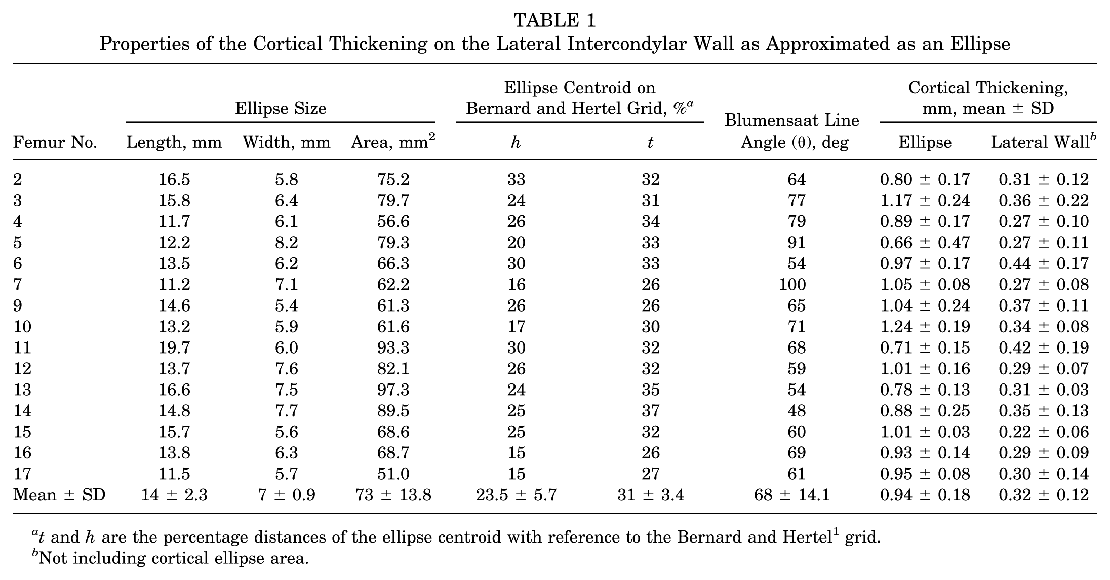
t and h are the percentage distances of the ellipse centroid with reference to the Bernard and Hertel¹ grid.

Not including cortical ellipse area.

Figure 4.

Mean and SD of cortical thickness in millimeters within both the cortical thickening ellipse and the remaining lateral intercondylar wall outside that boundary.

The ellipses approximating the cortical thickened region were then colored red at 90% transparency to allow the reader to appreciate the typical region of thickness, including its full variation within this sample (Figure 5B). Furthermore, within some of the thicker regions, there sometimes existed an even thicker area. Those areas were asymmetrically placed and most often occurred in the more proximal end of the areas of cortical thickness. A visual representation of these regions, mapped as a 90% transparent yellow ellipse overlaid onto Figure 5B, is presented in Figure 5C.

Figure 5.

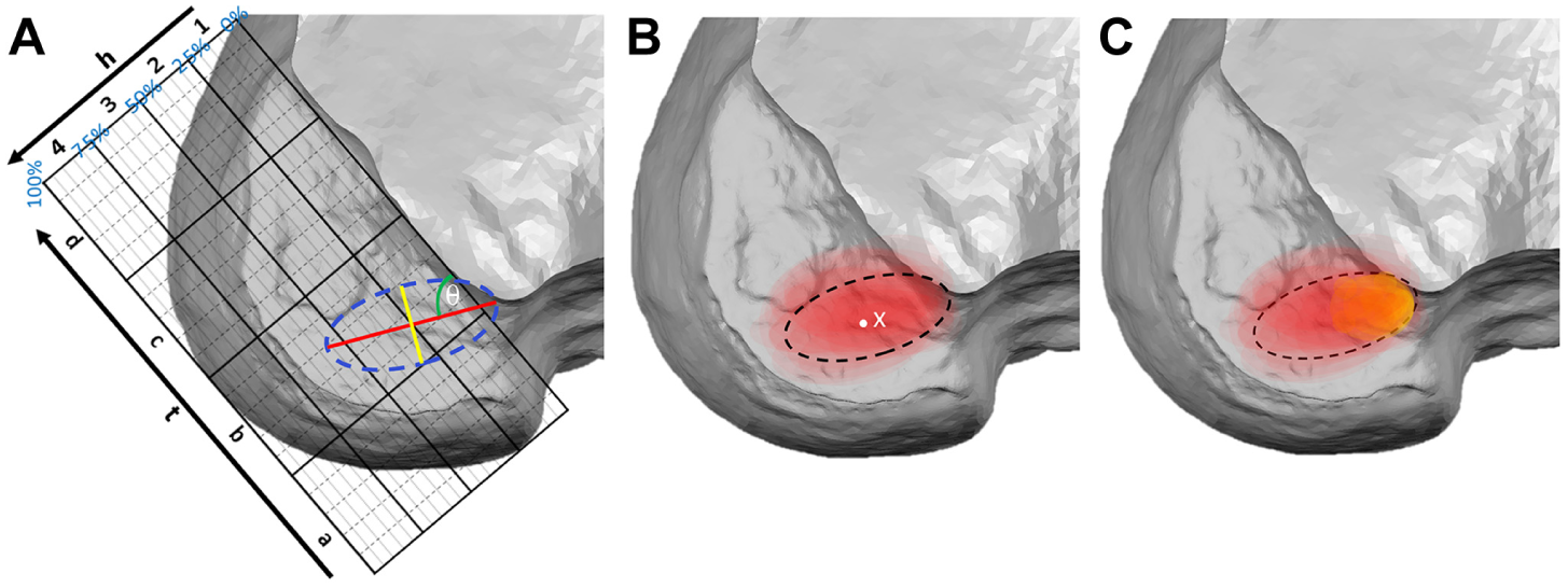
Overview diagram of each cortical thickening region as represented by a translucent ellipse, normalized and overlaid to provide a visual representation of where cortical thickening occurs. (A) Diagrammatic view of how the length (red), width (yellow), position (yellow/red intersection) of the ellipse (dashed blue line), and the Blumensaat line angle θ were measured from the Bernard and Hertel¹ grid shown; t and h are the percentage distances of the ellipse centroid, and 1-4/a-d are grid areas with reference to the Bernard and Hertel grid. (B and C) The dashed black line represents the average ellipse determined from all the ellipse geometric properties. (B) Only the significantly thicker regions compared with the rest of the lateral wall are shown; also shown is the mean centroid of all thickening ellipses (white X at 23.5 h:31 t) compared with the anatomic footprint of the ACL as reported in a recent systematic review²¹ (white dot 28.5 h:32.5 t). As well as the thicker region on the lateral wall, (C) highlights (yellow shading) the areas within this thick region that were again significantly thicker than the red region.

The high-resolution surface topology maps show the intercondylar ridge in all femurs to be present yet variable in its location, magnitude, and orientation, with no clear lateral bifurcate visible. Despite the objectiveness of the surface topology maps, colored based on relief (Figure 6), identifying the exact location of the lateral intercondylar ridge can be difficult and requires experience with this form of analysis.²⁰ Therefore, in Figure 7, we diagrammatically represent the location of the lateral intercondylar ridge (sometimes raised areas colored blue, sometimes step changes in height) to allow a clearer visual comparison between the surface topology and the regions of cortical thickening.

Figure 6.

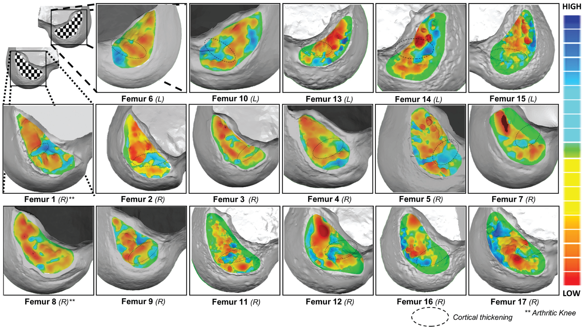
Relief surface topology maps of the lateral intercondylar wall overlaid with cortical thickening (represented by a dotted outline) for femurs in this study, with asterisks indicating whether femurs were arthritic.

Figure 7.

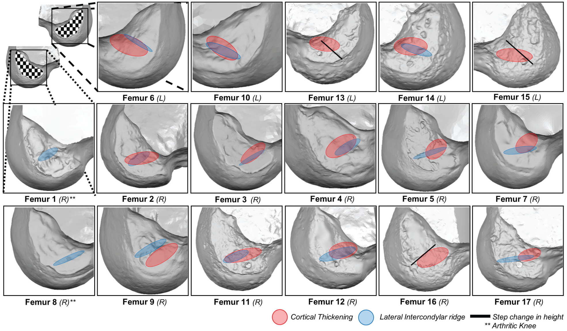
Diagram comparing our interpretation of the lateral intercondylar ridge on each femur (blue or red) against cortical thickening locations for each femur in this study, with asterisks indicating whether femurs were arthritic.

Discussion

In this study, we have identified areas of cortical thickening in the lateral femoral condyle consistent with the attachment of the ACL, which are on average 3 times thicker than the surrounding bone. The thickening found was similar in magnitude to that found in the histological study by Sasaki et al²² of the bone layer at the ACL insertion point. A different pattern was seen on the medial femoral condyle with cortical thickening seen much more anteriorly, consistent with the attachment of the posterior cruciate ligament. This indicates that the thickening is not simply a structural continuation of the thickening of the notch roof seen throughout in Figures 2 and 3 but rather due to the ligament attachments.

It has long been known that bone is highly responsive to the stresses placed upon it.^17,30 Recent studies have demonstrated that there is a linear response between local stress, bone mass, and cortical thickness.^3,25 Osteoblasts respond to the stress placed upon them on a microscopic level, and therefore adaptations to bone mass and thickness occur at localized sites of high stress and only at the specific location of that stress.^11,29 Given that bone is so responsive to the forces placed upon it, it is highly likely that the patterns observed in our study are due to the stresses on the bone resulting from the ligamentous attachments.²⁶ The areas of thickness can therefore be considered representative of the mechanically important components of the femoral footprint of the ligaments.³¹

The patterns observed are not the same as the total footprint of the ACL, which has been well described elsewhere, and clearly not all of the fibers of the ACL had a functional effect in these individuals. However, the distribution does appear to be consistent with emerging theories about the functional anatomy of the ACL, particularly the work of Iwahashi et al¹⁴ demonstrating that the ACL has “direct” and “indirect” fibers, as well as the ribbon concept popularized by Śmigielski et al.^22,24 Both of these concepts describe a group of more important fibers in a similar region as the area of cortical thickness described in the current study, and our data support the observation that the ACL soft tissue footprint is not universally loaded as indicated by the thickened regions in Figures 2 and 5.

The shapes observed in Figure 5 were defined by fitting an ellipse to the outline of the area of cortical thickening. While it is accepted that this method has its flaws in defining complex shapes, we believe it allowed a sufficient fit to the areas of thickening to define their size and location. The position, size, and orientation of the areas were therefore able to be documented and described on a Bernard and Hertel grid, allowing comparative data to be made to other studies before this, as well as in the future. The areas were, on average, 14 mm in length and 7 mm in width, with their mean centroid in a position of 23.5h: 31 t on the Bernard and Hertel grid (Figure 5B, white X), as opposed to the 28.5h: 32.5 t mean position identified in a recent systematic review for the anatomic footprint of the fibers²¹ (Figure 5B, white dot). In fact, the distribution of bone thickness within this region was not even, and thicker areas were generally seen higher up in the notch (proximal and posterior), implying that stresses in the ACL are greater in that region (Figure 5, B and C).

The ideal location for reconstruction of the femoral tunnel of the ACL remains under debate. Over the past 18 months, our technique has changed to position the tunnel closer to the soft tissue attachment of the anteromedial bundle. This study corroborates that approach, as the thickest areas of bone were seen at the most proximal end of the ellipse (Figure 5C), although the “perfect” position of the femoral tunnel is likely to vary from case to case and may require future research to individualize tunnel position to the functional anatomy of the patient.

By defining these areas, we are not attempting to suggest an ideal location for a drill tip to establish a femoral tunnel, however. It may be that the ideal shape to reconstruct the ACL is not circular at all or that the center of a tunnel should not overlie the most functional area, but that its leading edge is more functionally important. While more work is required to define the answers to those questions, it is clear that the functional footprint of the ACL can be defined, and work to optimize reconstructions to reproduce that anatomy in reconstructed patients would be recommended. It may be that identification of cortical thickness either preoperatively with CT or perioperatively using ultrasound would allow reconstructions to be tailored to the functional anatomy of the patient.¹⁸ Overall, a better understanding of the functionally important areas of the ACL is likely to lead to improvements in rupture rates, clinical outcomes, and knee biomechanics after reconstruction.¹⁰

We originally set out to examine the surface topography of the lateral femoral condyle to examine the use of surgical landmarks as reference points for the ACL, which have been found to be highly variable.²⁰ There does appear to be a relationship between the intercondylar ridge and the underlying areas of bone sclerosis, following on from previous descriptions of the ridge being part of the attachment point of the “direct” (or most functional) fibers of the ACL. However, that relationship is not entirely consistent; in some patients, the thickest parts were just anterior to the ridge, and in others it was posterior to the ridge (Figures 6 and 7). We therefore cannot recommend the intercondylar ridge as a landmark to guide ACL reconstruction, as the ridge does not correlate well enough with the functional attachment of the ligament to be correct for all patients.

The study has weaknesses that should be discussed. Because of the small sample size of this study, along with some of the samples belonging to matched pairs, the statistical power of this study is limited. While the sample size is relatively small, a consistent pattern could be observed throughout the 17 cases. There were 2 cases where an area of thickness could not be observed; however, these knees were both observed (independently assessed by a highly experienced ACL surgeon) to have significant macroscopic changes of osteoarthritis, which was not observed in the other 15 knees. It may be that the strain on the ACL reduces in osteoarthritis cases, resulting in the change of bony architecture in these knees compared with the rest of the group. Also, the samples were from older cadavers, and therefore the results in this study could in theory differ from the region of thickening found in younger or more active adults. While the stress-bone response is preserved in older adults, the overall bone mass may have reduced, or the usage of the knee may have changed slightly, and further work is planned to repeat this study in younger individuals. However, the anatomy of the ACL footprint is not considered to change throughout life and neither should its relative stress during activities of daily living. It is therefore highly likely that the findings from this study can be generalized to the wider population.

We had hoped to examine the soft tissue attachment of the ACL in relation to the bony anatomy and had included the use of magnetic resonance imaging (MRI) in this protocol. However, in practice, the resolution of MRI is far too low to match the degree of accuracy achieved using micro-CT, and other histological methods may be required in future studies. While concerns may be raised about the accuracy of CT in measuring cortical thickness, this is unlikely to be a problem in this study. Unlike a standard clinical scanner, our micro-CT system is able to achieve a resolution in the range of 70 to 90 μm, far below the sensitivity required to accurately identify and measure the thickness of the cortex in this region. The findings are therefore highly unlikely to represent a measurement error or artifact, although whether these areas could be identified using a clinical scanner or an intraoperative tool remains under investigation.

Conclusion

Overall, in this study we have identified a pattern of cortical thickening on the lateral wall of the intercondylar notch using high-resolution micro-CT, considered to represent the functional footprint of the ACL. This area is consistent with recent studies describing certain groups of fibers in the ACL that have differing functional importance. The area in which the thickening was found has been defined, but the relationship to the surface anatomy is variable. By looking at the subchondral microstructure, this study increases our understanding of the functional anatomy of the ACL and will help guide improvements in ACL reconstruction in the future.

Footnotes

Acknowledgements

This article is dedicated to Andrew Sprowson, MRCS (1975-2015), whose enthusiasm, dedication, and humor helped drive this research forward.

One or more of the authors has declared the following potential conflict of interest or source of funding: This research was funded through a grant from Smith & Nephew, enabling purchase of cadaveric specimens and use of the micro-CT scanner. T.J.W.S. has an educational contract with Smith & Nephew.

References

Bernard

Hertel

Intraoperative and postoperative insertion control of anterior cruciate ligament-plasty: a radiologic measuring method (quadrant method). Unfallchirurg. 1996;99:332-340.

Bird

Carmont

Dhillon

. Validation of a new technique to determine midbundle femoral tunnel position in anterior cruciate ligament reconstruction using 3-dimensional computed tomography analysis. Arthroscopy. 2011;27(9):1259-1267.

Christen

Ito

Ellouz

. Bone remodelling in humans is load-driven but not lazy. Nat Commun. 2014;5:4855.

Ciarelli

Fyhrie

Schaffler

Goldstein

SA.

Variations in three-dimensional cancellous bone architecture of the proximal femur in female hip fractures and in controls. J Bone Miner Res. 2000;15(1):32-40.

Doube

Kłosowski

Arganda-Carreras

. BoneJ: Free and extensible bone image analysis in ImageJ. Bone. 2010;47(6):1076-1079.

Dougherty

Kunzelmann

K-H.

Computing local thickness of 3D structures with ImageJ. Microsc Microanal. 2007;13(S02):1678-1679.

Ferretti

Ekdahl

Shen

FH.

Osseous landmarks of the femoral attachment of the anterior cruciate ligament: an anatomic study. Arthroscopy. 2007;23(11):1218-1225.

Ferretti

Levicoff

Macpherson

Moreland

Cohen

FH.

The fetal anterior cruciate ligament: an anatomic and histologic study. Arthroscopy. 2007;23(3):278-283.

Jordan

SS.

The lateral intercondylar ridge: a key to anatomic anterior cruciate ligament reconstruction. J Bone Joint Surg Am. 2007;89(10):2103-2104.

10.

Karlsson

A long journey to be anatomic. Knee Surg Sports Traumatol Arthrosc. 2010;18(9):1151-1153.

11.

Hambli

Connecting mechanics and bone cell activities in the bone remodeling process: an integrated finite element modeling. Front Bioeng Biotechnol. 2014;2:6.

12.

Hildebrand

Laib

Müller

Dequeker

Rüegsegger

Direct three-dimensional morphometric analysis of human cancellous bone: microstructural data from spine, femur, iliac crest, and calcaneus. J Bone Miner Res. 1999;14(7):1167-1174.

13.

Hildebrand

Rüegsegger

A new method for the model-independent assessment of thickness in three-dimensional images. J Microscopy. 1997;185(1):67-75.

14.

Iwahashi

Shino

Nakata

. Direct anterior cruciate ligament insertion to the femur assessed by histology and 3-dimensional volume-rendered computed tomography. Arthroscopy. 2010;26(9):S13-S20.

15.

Kopf

Musahl

Tashman

Szczodry

Shen

FH.

A systematic review of the femoral origin and tibial insertion morphology of the ACL. Knee Surg Sports Traumatol Arthrosc. 2009;17(3):213-219.

16.

McCalden

McGeough

Barker

MB.

Age-related changes in the tensile properties of cortical bone: the relative importance of changes in porosity, mineralization, and microstructure. J Bone Joint Surg Am. 1993;75(8):1193-1205.

17.

Meyer

Archief fur den anatomische und physiologischen Wissenschaften im Medizin. Die Architektur der Spongiosa. 1867;34:615-628.

18.

Muller

Moilanen

Bossy

. Comparison of three ultrasonic axial transmission methods for bone assessment. Ultrasound Med Biol. 2005;31(5):633-642.

19.

Nazarian

von Stechow

Zurakowski

Müller

Snyder

BD.

Bone volume fraction explains the variation in strength and stiffness of cancellous bone affected by metastatic cancer and osteoporosis. Calcif Tissue Int. 2008;83(6):368-379.

20.

Norman

Getgood

Thornby

. Quantitative topographic anatomy of the femoral ACL footprint: a micro-CT analysis. Med Biol Eng Comput. 2014;52(11):985-995.

21.

Piefer

Pflugner

Hwang

Lubowitz

JH.

Anterior cruciate ligament femoral footprint anatomy: systematic review of the 21st century literature. Arthroscopy. 2012;28(6):872-881.

22.

Sasaki

Ishibashi

Tsuda

. The femoral insertion of the anterior cruciate ligament: discrepancy between macroscopic and histological observations. Arthroscopy. 2012;28(8):1135-1146.

23.

Schneider

Rasband

Eliceiri

KW.

NIH Image to ImageJ: 25 years of image analysis. Nat Methods. 2012;9(7):671-675.

24.

Śmigielski

Zdanowicz

Drwięga

Ciszek

Ciszkowska-Łysoń

Siebold

Ribbon like appearance of the midsubstance fibres of the anterior cruciate ligament close to its femoral insertion site: a cadaveric study including 111 knees. Knee Surg Sports Traumatol Arthrosc. 2015;23(11):3143-3150.

25.

Sugiyama

Meakin

Browne

Galea

Price

Lanyon

LE.

Bones’ adaptive response to mechanical loading is essentially linear between the low strains associated with disuse and the high strains associated with the lamellar/woven bone transition. J Bone Miner Res. 2012;27(8):1784-1793.

26.

Sugiyama

Price

Lanyon

LE.

Functional adaptation to mechanical loading in both cortical and cancellous bone is controlled locally and is confined to the loaded bones. Bone. 2010;46(2):314-321.

27.

Tsukada

Fujishiro

Watanabe

. Anatomic variations of the lateral intercondylar ridge relationship to the anterior margin of the anterior cruciate ligament. Am J Sports Med. 2014;42(5):1110-1117.

28.

van Eck

Samuelsson

Vyas

van Dijk

Karlsson

FH.

Systematic review on cadaveric studies of anatomic anterior cruciate ligament reconstruction. Knee Surg Sports Traumatol Arthrosc. 2011;19(suppl 1):S101-S108.

29.

Webster

Wirth

van Lenthe

Müller

Experimental and finite element analysis of the mouse caudal vertebrae loading model: prediction of cortical and trabecular bone adaptation. Biomech Model Mechanobiol. 2012;11(1-2):221-230.

30.

Wolff

Das gesetz der transformation der knochen. DMW-Deutsche Medizinische Wochenschrift. 1892;19(47):1222-1224.

31.

Yeni

Brown

Wang

Norman

TL.

The influence of bone morphology on fracture toughness of the human femur and tibia. Bone. 1997;21(5):453-459.

32.

Ziegler

Pietrini

Westerhaus

. Arthroscopically pertinent landmarks for tunnel positioning in single-bundle and double-bundle anterior cruciate ligament reconstructions. Am J Sports Med. 2011;39(4):743-752.