Beyond Solow: Long-Run Growth in Intermediate Macroeconomics

Abstract

For decades the Solow model has been a workhorse in intermediate macroeconomics classrooms and textbooks. The explanatory power, analytic simplicity, and intuitive graphical exposition combine to make the model an indispensable part of the undergraduate macroeconomics canon. There is much less consensus on what, if anything, should be covered beyond the Solow model. Given that sustained economic growth has only occurred over the last two centuries, I argue that the Solow model should be part of a more comprehensive class module on economic growth. The module would begin with the logic of the Malthusian trap, move to the Solow model, and conclude with a model of endogenous technology growth. Some class time can also be devoted to the institutional, cultural, and geographic reasons that plausibly keep some countries in the Malthusian trap. Taken together, this module provides students with a comprehensive, yet accessible, view of macroeconomic history.

Keywords

O4 A22 economic education growth Solow

Introduction

Making sense of the upward sloping trend line in GDP per capita is a foundational topic in intermediate macroeconomics. The trend line is conventionally explained within the context of the Solow model. Combining a neoclassical production function with an equation describing the accumulation of physical capital is an accessible point of entry for undergraduate economics majors. Not only is it accessible, but the model is intuitive and provides empirically verifiable predictions. Quite naturally, the Solow model is in the undergraduate macroeconomics canon and I certainly do not advocate displacing it.

And yet, as Appendix Figure A1 shows in the case of the United Kingdom, sustained economic growth is a recent phenomenon.^1,2 Up until the Industrial Revolution the Malthusian trap (Malthus, 2024) dominated the world. A fixed supply of land combined with a positive income-fertility gradient implied that countries were stuck in a subsistence steady state. Notably, technological improvements in a Malthusian economy are, in the long run, eaten up by a larger population rather than sustaining a higher income per capita. I contend that some form of the Malthusian model should be taught in intermediate macroeconomics.

Teaching the Malthusian model confers a number of advantages to students. First, it helps them understand world economic history. It’s important to understand that sustained economic growth is a recent phenomenon that has taken hold in different countries at different times. Second, there exist pedagogical complementarities between the Malthusian and Solow models. They both feature neoclassical production functions with labor as one input and either land (Malthus) or physical capital (Solow) as the other input. The population growth equation in Malthus is analogous to the capital accumulation equation in Solow and the transition dynamics are conceptually similar. Essentially, conditional on having learned the Malthusian model, the Solow model is easier to understand. Third, the Malthusian model invites interdisciplinary perspectives from historians, anthropologists, and, if one is interested in discussing institutions, political scientists. Stock (2017) finds that economics is rising in popularity as a second major for US undergraduates, which suggests that a growing fraction of students would be receptive to interdisciplinary topics. Finally, the Malthusian model provides instructors with the opportunity to engage students with some interesting and unconventional datasets. The Maddison Project Database, which I used in creating Appendix Figure A1, is the most obvious example. With population and GDP per capita data going back 2,000 years, the Maddison data allows one to analyze the demographic and economic evolution of a subset of countries using either Stata or Microsoft Excel. In summary, and stipulating that one additional topic crowds out something else, I think the Malthusian model is an essential piece of intermediate macroeconomics.

In my experience, transitioning from the Malthusian world to the industrialized world, characterized by the Solow model, is an intuitive progression for students. They understand that the two ingredients necessary for the Malthusian trap are the existence of a fixed factor in production and the positive relationship between income and fertility. Changing either of these two assumptions breaks an economy free of the Malthusian trap. I cover a simplified version of Hansen and Prescott (2002) two-sector model to demonstrate how the sector with the fixed factor disappears asymptotically. As for the decoupling of income and fertility, I discuss elements of Galor (2011) unified growth theory which predicts that parents begin to invest in their children’s education once a certain technological threshold is met. The investment in education breaks the fertility-income connection. While the analytic complexity of unified growth theory is beyond the scope of an intermediate class, students understand the general idea. Once unshackled from its Malthusian chains, the economy is industrialized and trend growth is achieved, making the Solow model a good description of reality.

The Solow model is, for good reason, highly acclaimed. It’s straightforward to show students how the model’s steady-state predictions are confirmed in the data. The distinction between absolute and conditional convergence, which is vital in cross-country growth regressions, emerges naturally from the model. And yet, the model has well-known challenges. The first is that conventional development accounting exercises attribute the majority of cross-country income differences to total factor productivity, which is taken to be exogenous. Second, trend growth in output per worker comes through sustained growth in technology, which is likewise taken to be exogenous. Inspired by the misallocation and economic growth literature, summarized by Restuccia and Rogerson (2017), I present a simple model of input misallocation that leads to lower aggregate productivity. Discussing misallocation allows instructors to present interesting and important case studies such as input allocation in China and India (Hsieh & Klenow, 2009) and the macroeconomic effects of reducing discrimination in the United States (Hsieh et al., 2019).

Misallocation can, in a mechanical sense, explain why some countries have relatively low productivities. But the deeper causes of productivity differences, and economic growth more generally, are to be found at the historical nexus of politics, culture, and good luck. High-income countries have developed institutions that protect private property, enforce the rule of law, and encourage market competition. Some of them, out of sheer good fortune, also have favorable geographic endowments. After showing some of the cross-country correlations between these variables and income per worker, I refer readers to several of the seminal contributions in economic history that try to understand the mechanisms more deeply.

For a model of endogenous technological growth I turn to a simplified version of the Romer model. The key result is that the growth rate of technology along a balanced growth path is proportional to the population growth rate. A higher population goes from being a hindrance, as it is in the Malthusian model, to the key mechanism of sustained economic growth. In recent years I’ve concluded this section of class by discussing the future of economic growth, drawing from Jones (2022b) and Bloom et al. (2020). By starting with the Malthusian model and ending with the Romer model, this section of class—which, in my experience, takes about 4 weeks—can be thought of as an “almost unified growth theory.” Although the transitions between epochs occur endogenously in the genuine unified growth theory, the approach described in this article is more suitable for intermediate macroeconomics students.

All the intermediate macroeconomics textbooks that I’m aware of discuss the Solow model and most of them discuss some version of endogenous growth. Williamson (2017) has a section on the Malthusian model. My approach to endogenous growth is most aligned with Charles Jones’s semi-endogenous growth model which is discussed in his economic growth book coauthored with Jones & Vollrath (2023). The forthcoming second edition of my own textbook, Lester (2023), basically follows the progression from Malthus to Solow to endogenous growth.³ There is value in expanding our treatment of economic growth in intermediate macroeconomics. Sustained economic growth is an important part of human history and it’s easy to convince students of this. Indeed, they might even agree with Lucas (1988) that “once one starts thinking about economic growth, it is hard to think about anything else.” If your students stand a chance of becoming this mesmerized, it might be better to save economic growth for the last few weeks of class.

The Malthusian Economy

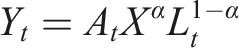
The Malthusian model is built on two key assumptions. The first is that output is produced with at least one fixed factor, which is conventionally assumed to be land. This isn’t difficult to justify historically; the vast majority of able-bodied adults were, prior to industrialization, working in agriculture. The production function is

Y_{t} = A_{t} X^{α} L_{t}^{1 - α}

where

Y_{t}

is GDP,

X

is land,

L_{t}

is labor,

A_{t}

is exogenous total factor productivity (TFP), and

0 < α < 1

is a curvature parameter. As the fixed factor, land is the only variable without a time subscript. Dividing by

L_{t}

transforms the production function into per-worker terms

y_{t} = A_{t} {(\frac{X}{L_{t}})}^{α} .

(1)

Output per worker, $y_{t}$ , is an increasing function of TFP and land per worker. Consistent with the Malthusian logic, an increase in population, all else equal, spreads land more thinly across workers, thereby reducing output per worker.

The population in the next time period (which one might think of as a decade or generation) is

L_{t + 1} = L_{t} + births - deaths .

(2)

I assume a constant mortality rate $d > 0$ and, following the Malthusian premise, a fertility rate that is increasing with income per worker. Defining $m_{t}$ as the average number of children born per adult, the fertility equation is

m_{t} = \frac{c}{p} y_{t}

(3)

where the parameters

p

and

c

can be thought of as the price and preference weight of children, respectively. This equation is what emerges from the micro-founded version of the model in Ashraf and Galor (2011).

The positive relationship between income and fertility during the Malthusian period is not as well established as the self-evident importance of land. Clark and Hamilton (2006) show that the number of surviving offspring listed in English wills during the 16th century increased with the testator’s assets. From this, Clark and Hamilton infer that wealthier men had more reproductive success. However, they cite studies with conflicting findings, and it isn’t immediately clear where the balance of the evidence lies. Murtin (2013), meanwhile, demonstrates that, controlling for education, fertility increases with income up to a certain level. Thus, the fertility-income relationship in equation (3) has some, though not unequivocal, empirical support.

Substituting equations (1) and (3) into (2) gives

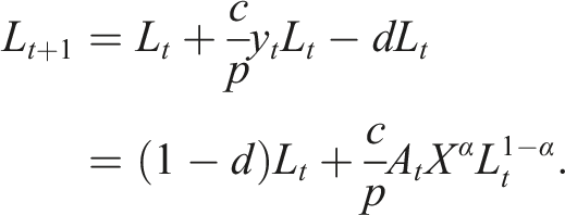
\begin{array}{l} L_{t + 1} & = L_{t} + \frac{c}{p} y_{t} L_{t} - d L_{t} \\ = (1 - d) L_{t} + \frac{c}{p} A_{t} X^{α} L_{t}^{1 - α} . \end{array}

Foreshadowing the Solow model, the population growth equation bears a striking resemblance to the capital accumulation equation. Population in the next period includes everyone who did not die in period $t$ , $(1 - d) L_{t}$ , plus new births, $m_{t} L_{t}$ . The Malthusian steady state is reached when the birth rate equals the death rate. The steady state and the associated transition dynamics can be understood by plotting the population growth equation against the 45-degree line as shown in Figure 1. $L_{t + 1}$ is a positive and concave function of $L_{t}$ . Moreover, it is straightforward to verify the Inada conditions ensuring that the population growth line crosses the 45-degree line at a unique positive steady state.

Figure 1.

The dynamics of population growth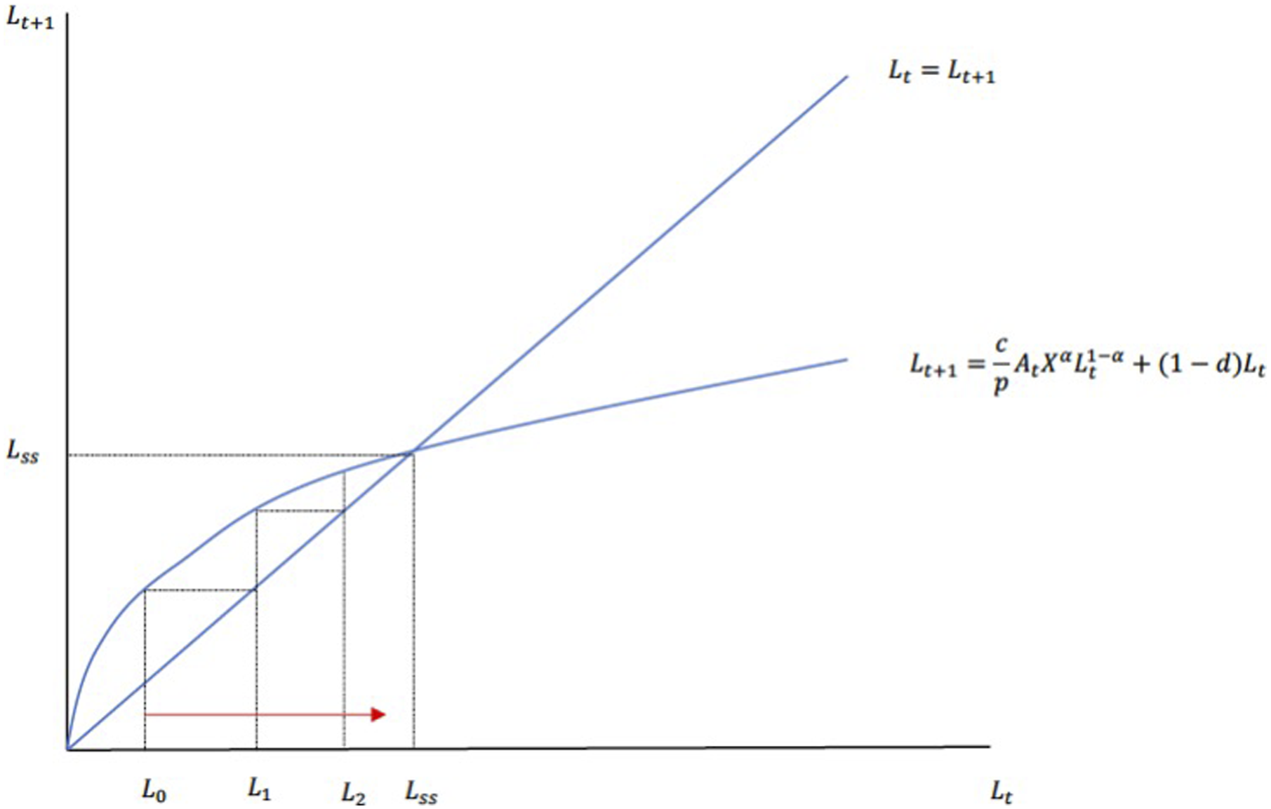

In steady state, the number of births equals the number of deaths and population is constant. If the economy starts with a relatively small population, at $L_{0}$ , for example, land and output per worker are high. The high level of output per worker results in a number of births that exceed the number of deaths and the population grows. As the population increases, land and output per worker fall. Although births still exceed deaths, the gap is smaller at $L_{1}$ than at $L_{0}$ . The dynamics continue to follow this logic until the population settles at steady state, $L_{s s}$ . The reverse, but conceptually identical, logic applies if the population starts above steady state.

A striking result in the Malthusian model is that a permanent increase in technology leaves long-run output per worker constant. This can be seen by evaluating the model in steady state. The model’s steady-state population and output per worker are given by

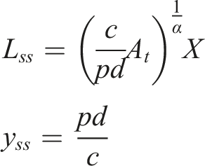
\begin{array}{l} L_{s s} & = {(\frac{c}{p d} A_{t})}^{\frac{1}{α}} X \\ y_{s s} & = \frac{p d}{c} \end{array}

respectively. Although technology doesn’t raise output per worker in the long run, it does boost it temporarily as shown in Figure 2. Starting in steady state, TFP jumps to a higher level at time $t_{0}$ . The left panel shows that population grows to a larger steady state. The right panel shows that income per capita initially jumps up to $y_{H T}$ , where “HT” stands for “high technology.” As the population grows over time, however, land per capita and output per capita start to decline. After the transition dynamics conclude, output per worker returns to its original steady state. Essentially, parents use the extra income to purchase more children and, in doing so, arrive at a new steady-state equilibrium that is denser but not richer.

Figure 2.

A one-time permanent increase in 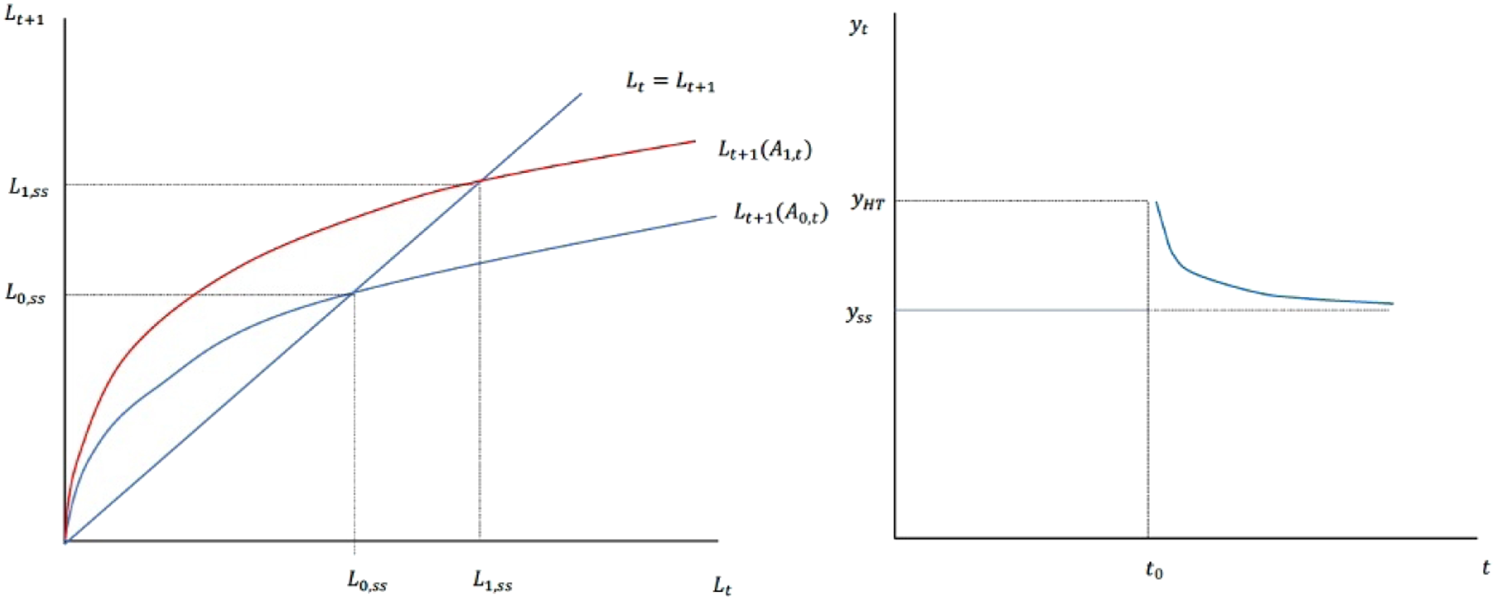$A_{t}$ in the Malthusian model

The steady-state equation for output per worker concisely captures the tragedy of the Malthusian economy. Societies with a high preference weight on children will be poorer, whereas societies in which kids are more costly or where mortality rates are higher will be richer. Clark (2008) eloquently summarizes the historical evidence supporting these predictions and others. I focus more narrowly on technology in class. Is it in fact true that more technologically sophisticated societies had roughly similar living standards to those of countries further from the frontier?

Empirically Evaluating the Malthusian Model

Research by Ashraf and Galor (2011) suggests that the answer to the last question is yes. Drawing on data from the Maddison Project Database, The Atlas of Cultural Evolution, and a measure of land productivity assembled by Michalopoulos (2012), Ashraf and Galor test the predictions of the Malthusian model. Specifically, countries with higher land productivity or more advanced technologies should have higher population densities, but not higher per capita incomes.

Because causality between population and technology runs both ways, their preferred measure of technology is the number of years elapsed since a given country started the Neolithic Revolution. This reflects Diamond (1997) hypothesis in Guns, Germs, and Steel that the first countries to undergo the Neolithic Revolution got a head start on economic development. The authors show that Diamond’s hypothesis is supported by the data; countries first to undergo the Neolithic Revolution tended to be more technologically advanced in the years 1, 1000, and 1500 AD. Ashraf and Galor (2011) observe that while population density is positively correlated with the number or years since the transition, there is essentially no correlation between GDP per capita and the years since the transition. Thus, the Malthusian predictions are supported by the data.

This paper fascinates students. Although the econometric analysis is too advanced for a typical college sophomore or junior, they understand the basic idea. It also appeals to students interested in other disciplines. Although Ashraf and Galor are both economists, they draw on historical and anthropological data. Diamond himself is an anthropologist. Finally, it is an example of economic modeling at its finest. The three-equation Malthusian model reasonably describes economic history from the Neolithic Revolution to the Industrial Revolution—about 3,000 years per equation!

Ironically, of course, Malthus was writing his treatise just as Western Europe was entering a new epoch. The first edition of An Essay on the Principle of Population was published in 1798 just as England was undergoing an Industrial Revolution. Students are naturally curious what led to the transition and, in my opinion, there is a simple and historically accurate way of explaining it.

Escaping the Malthusian Trap

Breaking free from the Malthusian trap requires either reducing the importance of land in production or decoupling income from fertility. There is abundant evidence that both have occurred historically. The share of employment in agriculture, and therefore the importance of land, has declined over time. Meanwhile, as technology grew more sophisticated, parents began investing in the education of their children. Once this threshold was reached, bursts in productivity led to parents investing in the quality of their children rather than increasing their fertility. The seminal contribution of Galor and Weil (2000) focuses on the human capital channel, whereas Hansen and Prescott (2002) focus on the transition from a Malthusian sector heavily dependent on land to a modern sector that doesn’t depend on land at all. Both papers are great, but Hansen and Prescott’s model is easier to teach. Accordingly, I teach a boiled-down version of their model in my intermediate class.

GDP is produced in the agricultural sector, denoted with an “AG” subscript, and the modern sector, denoted with an “M” subscript. Although it doesn’t necessarily have to be the case, it is easiest to think of the output produced by these sectors as perfect substitutes.⁴ The production functions are given by

\begin{array}{l} Y_{A G, t} & = A_{t} X^{α} L_{A G, t}^{1 - α} \\ Y_{M, t} & = A_{t} L_{M, t} \end{array}

respectively. Although I abstract from physical capital, the key is that output is constant returns to scale in reproducible factors in the modern sector. The total labor force is split between the modern and agricultural sectors,

L_{t} = L_{A G, t} + L_{M, t}

. It is also not necessary to assume TFP is equal across the sectors. To the extent that productivity growth was faster in the modern sector (e.g., through the invention of the steam engine), the economy will transition out of agriculture faster.

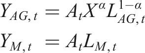
While not every student will have had calculus, most of them will be familiar with the concept of the marginal product of labor. In this model, an interior solution requires the marginal products of labor in the two sectors to equal each other:

1 = (1 - α) X^{α} L_{A G, t}^{- α} .

If $(1 - α) X^{α} L_{A G, t}^{- α} > 1$ then the entire labor force is allocated to agriculture. Otherwise, the optimal agricultural employment is constant at $L_{A G, t} = X {(1 - α)}^{\frac{1}{α}}$ . Intuitively, for economies beginning at the corner solution with $L_{A G, t} = L_{t}$ , a larger population reduces the marginal product of labor in agricultural. Once the population is large enough, the modern sector comes online and agriculture employment converges to a steady state. From that point on, all new labor goes into the modern sector.

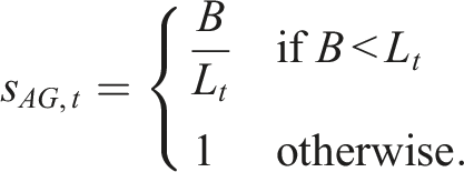
It is straightforward to solve the model at each point in time. In doing so, it’s convenient to write agriculture’s employment as a share of the labor force. Letting $B = X {(1 - α)}^{\frac{1}{α}}$ , the share of the labor force in agriculture, $s_{A G, t}$ , equals

s_{A G, t} = {\begin{cases} \frac{B}{L_{t}} & if B < L_{t} \\ 1 & otherwise . \end{cases}

Once the modern sector becomes operational, the number of workers in agriculture is constant and the agricultural sector, as a share of overall employment, declines over time. I initiate the model starting in year 1 AD. Data from McEvedy and Jones (1978) shows that the world’s population was about 170 million in 1 AD and about 610 million by 1700 which I take as the date the world started to industrialize.⁵ Given the annualized growth rate of 0.075%, I calibrate B so that the world starts to industrialize in 1700.

The time path of agriculture’s share is shown by the solid blue line in Figure 3. The model generates the correct qualitative pattern as the share of the labor force in agriculture declines over time. However, by 2000, close to 80% of the world’s adult population is predicted to work in agriculture, about twice as much as in the data. One way of dealing with this is to adjust the population growth rate. It is well known that global population growth accelerated during the most recent centuries as economies escaped the Malthusian trap. World population grew from about 600 million people in 1700 to about 1.6 billion in 1900, or 0.5% growth per year. The dotted red line shows the employment dynamics assuming that the population growth rate increases to 0.5% in 1700. By 2000, the predicted share of employment in agriculture is about 25%, much closer to historical averages.

Figure 3.

Predicted employment in agriculture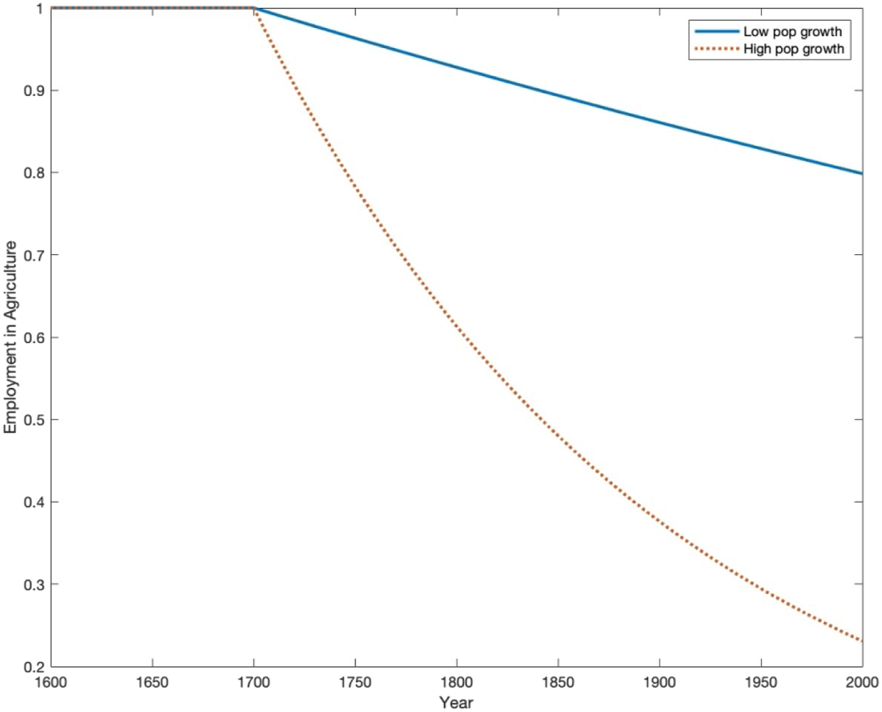

In summary, small but continuous population growth can lead economies to escape the Malthusian trap. The key, as observed by Hansen and Prescott, is that the economy has access to a latent sector that produces output independent of land. The migration from farms to cities is a great way to illustrate this in class. Instructors interested in discussing the role of human capital can show historical trends in literacy, school attendance, and educational attainment, rather than jumping into a full-blown quantity-quality model. The transition to the modern sector and the decoupling of fertility from income by way of human capital investment are both historically important phenomena and, ultimately, complement each other. Once the economy leaves the Malthusian trap, we can turn to a model of physical capital accumulation.

Two Cheers for the Solow Model

Macroeconomics instructors are well-versed in the Solow model. It appears in all intermediate textbooks that I’m aware of, albeit with different levels of mathematical sophistication. The acclaim is well deserved; the Solow model is a tractable dynamic model of economic growth that makes empirically verifiable and accurate predictions. A key lesson is that long-run economic growth is independent of a country’s investment rate. Students find this claim counterintuitive, but they easily grasp the logic once they understand the concavity of the production function. In my view, the Solow model’s place in the canon is well deserved, but students need to be aware of its limitations.

My version of the model is described by a production function and capital accumulation equation:

\begin{array}{l} Y_{t} & = A_{t} K_{t}^{α} {(h_{t} L_{t})}^{1 - α} \\ K_{t + 1} & = s Y_{t} + (1 - δ) K_{t} . \end{array}

Y_{t}

is GDP,

K_{t}

is physical capital,

A_{t}

is exogenous TFP, and

h_{t}

is exogenous human capital. Human capital is proportional to average educational attainment and is disciplined by the annual rate of return to education.⁶

0 < s < 1

is the savings rate,

0 < δ < 1

is the depreciation rate, and

0 < α < 1

is the elasticity of output with respect to capital. Because capital and labor are reproducible, the production function has constant returns to scale in rival inputs. This is in contrast to the Malthusian model where the aggregate quantity of land is fixed. Dividing the production function by

L_{t}

converts output into its per-worker counterpart:

y_{t} = A_{t} h_{t}^{1 - α} k_{t}^{α} .

(4)

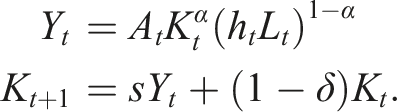
Another key distinction relative to the Malthusian model is that population growth is exogenous and independent of income. Letting the population growth rate equal $n$ , the capital accumulation equation in per-worker terms is

k_{t + 1} = \frac{1}{1 + n} [s A_{t} k_{t}^{α} h_{t}^{1 - α} + (1 - δ) k_{t}] .

(5)

To see the difference between the Malthusian model, consider a permanent, one-time increase in $A_{t}$ . The left panel of Figure 4 shows that the capital accumulation line shifts up and to the left. Over time, capital per worker increases from $k_{0, s s}$ to $k_{1, s s}$ . The panel on the right shows that, even holding the capital stock constant at $k_{0, s s}$ , output per worker jumps on impact because workers are more efficient at using the existing capital stock. As the economy accumulates more capital, output per worker continues to rise until the new steady state, $y_{1, s s}$ . Thus, unlike the Malthusian model, a more technologically advanced society will, in the long run, be richer in the Solow model.

Figure 4.

A one-time increase in 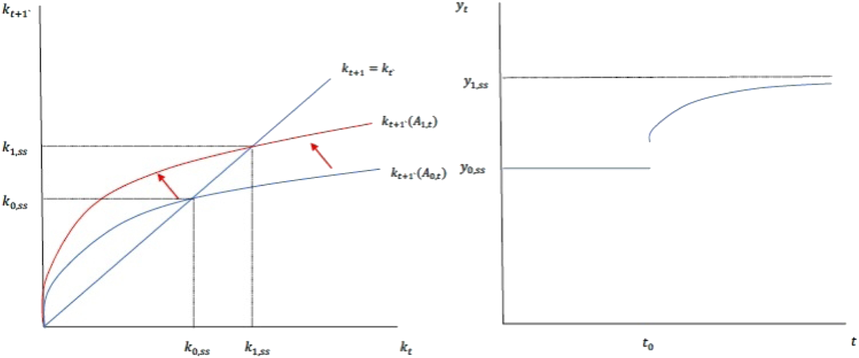$A_{t}$ in the Solow model

The Solow model can also be used for development accounting exercises. Letting $Z_{t} = A_{t}^{\frac{1}{1 - α}}$ , which is a convenient change of variables, and multiplying both sides of equation (4) by $y_{t}^{- α}$ results in

y_{t} = Z_{t} h_{t} {(\frac{k_{t}}{y_{t}})}^{\frac{α}{1 - α}} .

(6)

Output per worker is increasing in TFP, human capital, and the physical capital-to-output ratio.⁷ To understand the long-run predictions of the model, we can impose the steady state in equation (5):

\begin{array}{l} k_{s s} (1 + n) & = s y_{s s} + (1 - δ) k_{s s} . \end{array}

Solving for

\frac{k_{s s}}{y_{s s}}

gives

\frac{k_{s s}}{y_{s s}} = \frac{s}{n + δ} .

Finally, using equation (6), output per worker in steady state is

y_{s s} = Z_{t} h_{t} {(\frac{s}{n + δ})}^{\frac{α}{1 - α}} .

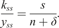
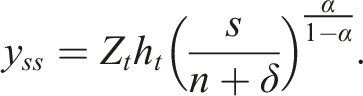
Over long time horizons, countries with higher savings rates, lower population growth rates, and higher levels of human capital and TFP are predicted to be richer. Appendix Figure A2 shows that all four of these predictions are empirically supported. I use data from the Penn World Tables, Feenstra et al. (2015), which is straightforward to download into Stata or Excel. It is also available in the Federal Reserve Bank of Saint Louis FRED database.

Appendix Figure A3 shows that the Solow model is directionally correct in its long-run predictions. It also makes valuable predictions regarding convergence. The Solow model predicts that countries will converge to the same level of income per worker if and only if they have the same steady states. A corollary is that countries furthest below their steady states will grow the fastest. The top panel of Appendix Figure A3 shows that the evidence in favor of unconditional convergence — initially poor countries catching up to initially rich countries — is quite weak. The evidence in favor of conditional convergence, on the other hand, is stronger as shown in the bottom panel. The scatter plot shows the relationship between income per capita relative to steady state (on the horizontal axis) and cumulative growth between 1970 and 2019. The negative correlation is exactly what is implied by the conditional convergence hypothesis.

The qualitative steady-state predictions and the conditional convergence hypothesis are two points going in the Solow model’s favor. Moreover, it is not complicated to add variable employment, government spending, and alternative forms of human capital accumulation to the model. In sum, the Solow model is an indispensable part of the macroeconomics curriculum.

The quantitative predictions are a different matter. Equation (6) can be used in a development accounting exercise. One of the reasons I write output per worker as a function of the capital-to-output ratio rather than capital per worker is that the former is invariant to TFP along a balanced growth path. That makes it easier to disentangle differences in per capita income coming from TFP rather than from differences in savings rates.⁸ Using the United States as the reference country, the development accounting equation is

\frac{y_{U S}}{y_{i}} = \frac{Z_{U S}}{Z_{i}} \frac{h_{U S}}{h_{i}} {(\frac{\frac{K_{U S}}{Y_{U S}}}{\frac{K_{i}}{Y_{i}}})}^{\frac{α}{1 - α}} .

(7)

Equation (7) says that differences in output per worker are attributed to either (i) differences in TFP, (ii) differences in human capital, or (iii) differences in the capital-to-output ratio. Table 1 breaks down the numbers in 2019.⁹ Taking the second row as an example, income per worker is 26% higher in the US than in France. TFP and human capital are respectively 46% and 16% higher in the US; the scaled capital-to-output ratio is 26% lower in the United States. On the whole, income per capita is 237% higher in the US than in the median country. Because the savings rate in the United States is lower than the global average, the capital-to-output ratio reduces the income spread between the United States and the rest of the world.

Table 1.

Sources of cross-country income differences in 2019

Country	Income	Human capital	Physical capital	TFP
Norway	0.95	1.02	0.87	1.07
France	1.26	1.16	0.74	1.46
Japan	1.81	1.04	0.80	2.15
China	5.16	1.39	0.82	2.15
India	7.07	1.73	0.93	4.39
Brazil	3.97	1.21	0.87	3.76
Zambia	11.95	1.39	0.79	10.80
Zimbabwe	21.61	1.41	1.38	11.10
Median	3.37	1.35	0.90	2.65

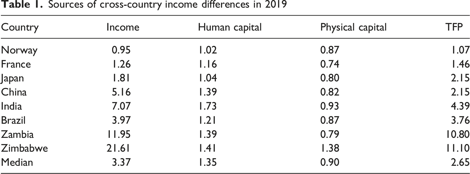
TFP accounts for more than three-quarters of difference between US income and the global median, while human capital accounts for another 25%. The punchline from this accounting exercise is that differences in living standards are driven by differences in TFP and human capital accumulation, both of which are exogenous. What is needed, as recognized as far back as Abramovitz (1956), is a theory of endogenous TFP.

After spending multiple classes analyzing the Solow model, students are understandably deflated by this conclusion. The instructor has two options. One is to forge ahead with theories of endogenous TFP. Another is to distinguish the proximate causes of economic growth (factor accumulation) from the deep causes (culture, geography, political institutions). Time constraints imply that students get at best a sampling of these theories, but spending a small portion of class time on them is well worth it. Devoting even one or two classes to the topics in the next section gives students a foretaste of political economy, causal regression analysis, and macroeconomic development.

Endogenous TFP

The first part of this section analyzes TFP differences within the cross-section. Next, I distinguish between proximate and deep causes of growth and discuss how the latter provides the foundational infrastructure for the former. The final part of this section analyzes the growth in TFP at the frontier. In other words, the first half asks why some countries lag so far behind the technological frontier, while the second half asks what moves the technological frontier forward.

Cross-Sectional TFP Differences

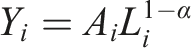
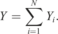
I focus on the misallocation theories of TFP, which go at least as far back as Restuccia and Rogerson (2008). Restuccia and Rogerson (2017) provide a literature review. Consider an economy with $N > 0$ firms where $N$ is exogenous. Each firm produces with the production function

Y_{i} = A_{i} L_{i}^{1 - α}

where

0 < α < 1

is a scaling parameter and

A_{i}

is firm-specific TFP. By assuming the firm-level production function has decreasing returns to scale, the model generates a non-degenerate size distribution of firms. Assuming the firms produce a homogeneous good, the economy’s GDP is

Y = \sum_{i = 1}^{N} Y_{i} .

The aggregate labor force is normalized to $\bar{L}$ so that $\sum_{i = 1}^{N} L_{i} = \bar{L}$ .

The marginal product of labor for firm $i$ is

{MPL}_{i} = (1 - α) A_{i} L_{i}^{- α} .

The marginal product of labor is increasing in TFP and decreasing in labor. Although some students will not be familiar with a social planner’s problem, it is easy to convince them that economic efficiency entails equating marginal products. If 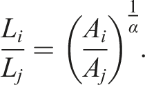${MPL}_{i} > {MPL}_{j}$ one could increase GDP by reallocating labor away from firm $j$ towards firm $i$ . Equating marginal products implies

\frac{L_{i}}{L_{j}} = {(\frac{A_{i}}{A_{j}})}^{\frac{1}{α}} .

An implication is that more productive firms should employ more workers; indeed, the returns-to-scale parameter magnifies firm-size differences. If $α = 0.5$ , a 10-fold difference in productivity would imply a 100-fold difference in the efficient level of employment.

As a concrete example, suppose $N = 2$ , $\bar{L} = 100$ , $α = 0.5$ , $A_{1} = 5$ , and $A_{2} = 10$ . Aggregate TFP in this economy is

\begin{array}{l} TFP & = \frac{Y_{1} + Y_{2}}{\bar{L}} \\ = \frac{5 L_{1}^{0.5} + 10 L_{2}^{0.5}}{100} . \end{array}

The optimal allocation of labor is

L_{1} = 20

and

L_{2} = 80

. Table 2 shows how alternative allocations affect GDP and aggregate TFP. Going from the optimal allocation to an equal split of labor reduces GDP and aggregate TFP by about 5%. While this figure is small compared to the massive variation in TFP displayed in Table 1, the example merely illustrates the point that the distribution of resources matters for aggregate TFP. Endogenous capital accumulation would amplify these differences over time as less productive firms accumulate more capital than would be optimal.

Table 2.

Example of Misallocation

$L_{1}$	$L_{2}$	GDP	TFP
20	80	111.8	1.11
35	65	110.2	1.10
50	50	106.1	1.06
65	35	99.5	1.00
80	20	89.5	0.90

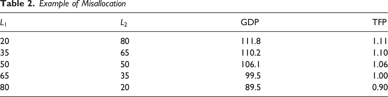
In addition to developing theories of misallocation over the last two decades, economists have also measured the extent to which resources are misallocated across countries. Perhaps the best-known paper is Hsieh and Klenow (2009), who document the size distribution of firms in India, China, and the United States. They show that the variance of firm size in all three countires is lower than what the efficient solution would imply, with the deviations from the efficient allocations being larger in China and India than in the US. Hsieh and Klenow estimate that moving to the US level of efficiency would raise TFP by 30–50% in China and 40–60% in India.

There are many contributors to misallocation. Hsieh and Klenow focus on the role of state-owned enterprises in China and the role of licenses and other regulations in India. Financial frictions can also misallocate resources across producers. In countries with under-developed financial markets poor but talented entrepreneurs can’t meet the collateral constraints necessary to obtain funding for their projects. When financial capital is not allocated to the most talented producers, aggregate TFP falls. While there is debate about the aggregate consequences of financial frictions, they certainly play some role in generating cross-country TFP differences.

If things were as simple as choosing good economic policy, why wouldn’t the entire world simply converge to the best policies? Mountains of scholarship in political science and economics have studied the deep causes of economic development. The next section provides a very brief sketch of these theories suitable for an intermediate class.¹⁰

Deep Causes of Economic Growth

Why have some countries successfully accumulated physical and human capital and efficiently allocated resources? One school of thought, exemplified by Jeffrey Sachs, is that geography plays a key role in development.¹¹ According to this view, tropical countries close to the equator face a higher disease burden and have inferior agricultural endowments. The left panel of Appendix Figure A4 shows that GDP per capita is higher in countries further away from the equator, which is consistent with Sachs’s logic. The burdens of economic geography cause some economies to lag behind in accumulating the factors of production. In this line of thought, geography is an important deep cause of economic growth.

An alternative perspective is that differences in institutions and quality of governance are the ultimate driving force of economic development. The middle panel of Appendix Figure A7 shows the relationship between a country’s economic freedom index (as constructed in the Fraser Institute’s “Economic Freedom of the World” Gwartney et al. (2025) and GDP per capita. The freedom index is intended to summarize a country’s rule of law, protection of property rights, soundness of money, and related variables with one number. Countries with better institutions earn a higher score and, as the figure demonstrates, a higher score is associated with a higher level of GDP per worker.

Yet, another perspective is that economic performance is driven by cultural variables. The World Value Survey constructed by Inglehart et al. (2017) conducts interviews in countries across the world. One question the survey asks is whether one agrees with the statement, “most people can be trusted.” The rightmost panel of Appendix Figure A4 shows that the percentage of people in a country answering yes to that question is positively related to living standards. One possible economic explanation is that transacting is easier in societies where people trust each other. The WVS has many other questions about religion, preferences for work and thrift, child rearing, and other topics.

Simply motivating a class with something like Appendix Figure A4 leads to a number of possible directions. I’ll elaborate on three. First, one can discuss the economic mechanisms through which the rule of law and protection of private property affect economic development. For instance, a lack of contract enforcement gives rise to financial constraints, which (as the last section discussed) leads to lower TFP. A government that fails to protect private property induces economic actors to divert resources away from productive activities and into personal security. A corrupt bureaucracy entices talented people away from entrepreneurship and into rent-seeking activities. Or, to tie culture back into it, a government that is ineffective at stopping crime reduces social trust. Then, GDP is lower because of the direct effect of crime and the indirect effect operating through social trust. One can even go so far as discussing why these inefficient policies persist. Or to use Acemoglu (2003) question, why is there no political Coase Theorem? Sketching an answer to this takes one into the realm of political economy which, after providing students a bit of a teaser, is a good off-ramp for this part of the class.¹² The connection between geography and per-worker income might be approached from a micro-development angle. More specifically, an instructor can discuss how climate, access to waterways, and prevalence of disease come to affect resource allocation. Although this is a macroeconomics class, students can get an idea of what an upper-level economic development class might look like.

The second direction to take the class is a discussion on identifying causal relationships. Identifying the causal relationship between institutions and economic performance is a formidable challenge. Before any regressions are run, even defining and measuring institutions are difficult. Do institutions include economic policies or should institutions be exclusively defined upstream of policy (i.e., institutions are rules about rules)? Are institutions best measured as an index value or as a categorical variable (e.g., political party)? Once a definition and a standard of measurement are agreed to, the complexity of establishing a convincing causal relationship begins. Most students in intermediate macro will not have taken econometrics, but it’s not difficult to discuss the cleverness of Acemoglu et al. (2001) settler mortality instrumental variable and why it is so contentious. While defining and measuring geographic variables might be more straightforward than institutional ones, inferring causality is perhaps just as challenging. For instance, do geographic variables operate through institutions, as Easterly and Levine (2003) argue, or do they exert an independent effect on economic development, as Sachs contends?

Finally, one can discuss how the institutional and geographic explanations aren’t mutually exclusive. Indeed, the more sophisticated theories posit that the two are subtly connected. Acemoglu et al. (2001) argue that favorable disease environments in former colonies encouraged European settlers to establish inclusive institutions, while poor disease environments led to extractive institutions. Similarly, Engerman and Sokoloff (2000) emphasize the role resource endowments played in shaping participatory political institutions. Colonies in Central and South America that were heavily endowed with native labor or were suitable for large plantation farming were run by a small elite that had a vested interest in limiting access to political power. The political institutions formed in the colonial period have persisted through time. As an example of historical roots of trust, Nunn and Wantchekon (2011) show that individuals whose ancestors were heavily raided in the African slave trade are less trusting today. Thus, the mechanism is that historical kidnapping and violence lead to persistently low levels of trust, which continue to affect economic development today.¹³ One can find many more examples of the nuanced dance between institutions, culture, geography, and economic performance.

Macroeconomic development is inherently historical and tends to be interdisciplinary, which is all to the benefit of students. Moreover, historical episodes occasionally allow economists to better understand causal mechanisms and how they propagate over time. To conclude the entire economic growth section of the class, I prefer to return to the present day and ask what drives economic growth at the frontier. From there, we can tentatively forecast the future of economic growth.

Technology Growth

The distinction between “TFP” and “technology” starts to matter when discussing growth at the frontier. TFP is anything that affects the efficiency of transforming inputs into output. Technology is, of course, one factor. More advanced technology raises a country’s TFP. But improved resource allocation also increases TFP. Because any decentralized resource allocation can’t be superior to the efficient solution, reducing misallocation results in a temporarily, but not permanently, higher growth rate in TFP. Sustained growth, on the other hand, must come from improvements in technology. A simplified version of the Romer (1990) model or Aghion and Howitt (1992) model is the right tool for this job in an intermediate class.

I start this section of class by deriving a balanced growth path. Referring back to equation (6), neither the capital-to-output ratio nor the time spent in school can be growing on a balanced growth path. It follows that the growth rate of output per worker equals the growth rate of $Z_{t}$ , which we can think of as technology.

I’ve had students read the first two sections of Romer (1990), who eloquently discusses the roles of rivalry, increasing returns, and imperfect competition in a brilliant yet digestible way. This is to convince students that the nonrivalry of ideas makes them unlike other goods and services. It also convinces them that assuming constant returns to scale in rival factors implies that either creators of ideas receive no compensation or there must be imperfect competition. Since the first possibility is directly contradicted by the data, Romer (1990) and most endogenous growth models that followed him assume imperfect competition.

While this is essential intellectual background for understanding endogenous growth theory, the heart of the model in an intermediate class is the idea production function.¹⁴ I follow the “semi-endogenous” approach pioneered by Jones (1995) which is better empirically supported than the idea production function in the original Romer model. Let $Z_{t}$ be the stock of ideas at time $t$ . The invention of new ideas is a function of the existing stock and the number of researcher scientists $L_{R, t}$ . Mathematically, the function is

Z_{t + 1} = Z_{t} + L_{R, t} Z_{t}^{b}

where

b < 1

. The parameter

b

governs the degree to which ideas build on each other. If

b > 0

then ideas get easier to discover over time. Jones and Vollrath (2023) call this the “standing on shoulders” effect. Conversely, if

b < 0

, the low-hanging fruit gets taken first and ideas get harder to find. Assuming a constant fraction of the population,

s_{R}

, is employed in research, the idea accumulation equation can be written as

\frac{Z_{t + 1} - Z_{t}}{Z_{t}} = \frac{s_{R} L_{t}}{Z_{t}^{1 - b}} .

(8)

The left-hand side of equation (8) is the growth rate of ideas. A balanced growth path requires that

Z_{t}

grow at a constant rate, which in turn implies that the numerator and denominator on the right-hand side must grow at the same rate. Assuming that the population growth rate remains constant at

n

, the growth rate of ideas is

g_{z} = \frac{n}{1 - b} .

(9)

Remarkably, the growth rate of ideas is proportional to the growth rate of the population. This result follows from the nonrivalry of ideas. Once calculus is invented, one student’s use of calculus doesn’t diminish any other student’s use of calculus. Another result of equation (9) is that the growth rate of technology on a balanced growth path is independent of the share of research scientists. This contrasts with the original Romer model, which includes such scale effects. Jones (1995) convincingly argues that the time-series data do not support scale effects. Bloom et al. (2020) show that the annual rate of US TFP growth has, if anything, fallen over time despite more than a 10-fold increase in research scientists. Bloom et al. (2020) document extensive evidence that ideas are getting harder to find in a number of economic sectors. They estimate that $b \approx - 2$ at the level of the aggregate economy.

Equation (8) is amenable to graphical analysis.¹⁵ Specifically, if $b = 0$ then the growth rate of ideas, $g_{z, t}$ , is a linear function of $\frac{s_{R} L_{t}}{Z_{t}}$ . Figure 5 shows the effects of a permanent one-time increase in the share of research scientists. On impact, the number of research scientists increases relative to the stock of ideas, which shifts the idea growth line to the left and pushes $g_{z, t}$ from $n$ to $g_{z, high}$ . As the denominator in $\frac{s_{R} L_{t}}{Z_{t}}$ grows faster than the numerator, the growth rate of ideas returns to $n$ and the economy settles at a permanently lower ratio of $\frac{L_{t}}{Z_{t}}$ . Thus, an increase in the share of researchers permanently increases the stock of ideas, but only temporarily increases the growth rate of ideas. This is analogous to an increase in the savings rate in the Solow model, which is one reason why this graph is pedagogically useful.

Figure 5.

An increase in the share of research scientists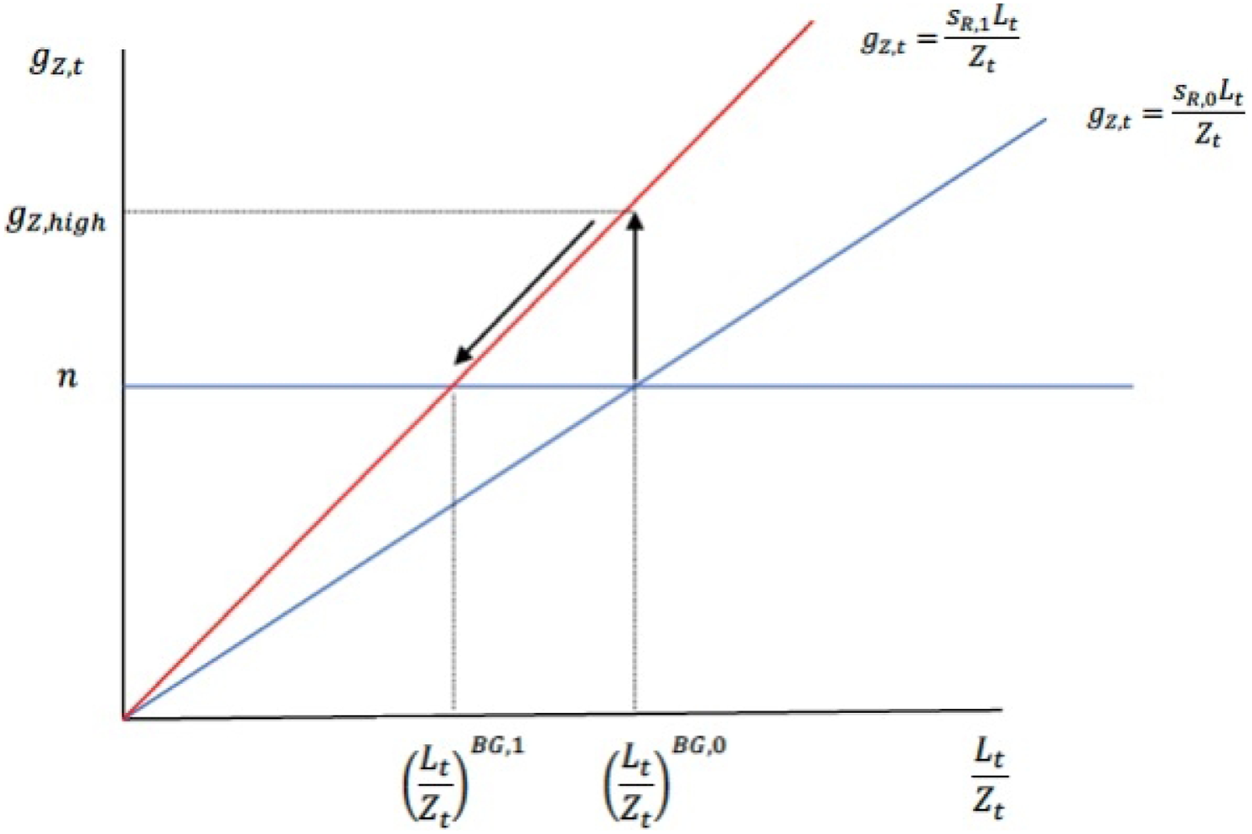

Endogenous growth theory is an appropriate bookend to a section on economic growth that began with the Malthusian model. The textbook and Marginal Revolution author Alex Tabarrok says there are two views of humanity: people are brains or people are stomachs. The Malthusian model is an obvious example of the latter. More people grazing over a fixed amount of land drag income per capita down. In the “people are brains” view, a bigger population means more ideas and, given their nonrivalry, all of humanity can benefit from them. Concluding this section of a class with endogenous growth also invites students to further inquiry along two dimensions. First is the decline in fertility rates below replacement levels in high-income countries. Jones (2022a) shows that a shrinking population eventually leads to an “empty planet” and a stationary stock of ideas. Second is the advent of artificial intelligence, which could fundamentally change the relationship between population and technology. The issues of fertility and artificial intelligence can be taken up in more advanced elective classes.

Conclusion

What explains the “hockey stick” graph in Appendix Figure A1 is one of the most important questions in social science. Economists have made enormous progress towards explaining the Malthusian trap, the transition to the modern growth regime, persistent inequality in living standards, and economic growth at the frontier. Given their importance, these intellectual breakthroughs should be taught at the intermediate level. This article shows how to suitably adapt some of the technical models to a level appropriate for undergraduate majors. The end result is an “almost unified growth theory” that can be taught in about a month. Students who want to explore the topic in more depth can take an economic growth elective in their junior or senior years.

Supplemental Material

Supplemental material - Beyond Solow: Long-Run Growth in Intermediate Macroeconomics

Supplemental material for Beyond Solow: Long-Run Growth in Intermediate Macroeconomics by Robert Lester in The American Economist

Footnotes

Acknowledgments

I’m grateful for comments from Christopher Foote, Michael Donihue, Roisin O’Sullivan, Diego Mendez-Carbajo, and the participants at the American Economic Association’s 2026 meeting.

ORCID iD

Robert Lester

Funding

The author received no financial support for the research, authorship, and/or publication of this article.

Declaration of Conflicting Interests

The author declared no potential conflicts of interest with respect to the research, authorship, and/or publication of this article.

Supplemental Material

Supplemental material is available online.

Notes

Author Biography

Robert Lester is an Associate Professor of Economics and a Haynesville Project Fellow at Colby College. He is the author of Macroeconomics: Theory and Applications published by Cengage and the coauthor with Julio Garı́n and Eric Sims of the open-source textbook Intermediate Macroeconomics.

References

Abramovitz

(1956). Resource and output trends in the United States since 1870. In: Resource and output trends in the United States since 1870 (pp. 1–23). NBER.

Acemoglu

(2003). Why not a political coase theorem? Social conflict, commitment, and politics. Journal of Comparative Economics, 31(4), 620–652. https://doi.org/10.1016/j.jce.2003.09.003

Acemoglu

Johnson

Robinson

J. A.

(2001). The colonial origins of comparative development: An empirical investigation. American Economic Review, 91(5), 1369–1401. https://doi.org/10.1257/aer.91.5.1369

Aghion

Howitt

(1992). A model of growth through creative destruction. Econometrica, 60(2), 323–351. https://doi.org/10.2307/2951599

Ashraf

Galor

(2011). Dynamics and stagnation in the malthusian epoch. American Economic Review, 101(5), 2003–2041. https://doi.org/10.1257/aer.101.5.2003

Bloom

Jones

C. I.

Van Reenen

Webb

(2020). Are ideas getting harder to find? American Economic Review, 110(4), 1104–1144. https://doi.org/10.1257/aer.20180338

Bolt

van Zanden

J. L.

(2020). Maddison style estimates of the evolution of the world economy: A new 2020 update. Groningen growth; Development Centre; Maddison Project Database. version 2020. https://www.rug.nl/ggdc/historicaldevelopment/maddison/releases/maddison-project-database-2020

Broadberry

Campbell

B. M.

Klein

Overton

Van Leeuwen

(2015). British economic growth, 1270–1870. Cambridge University Press.

Clark

(2008). A farewell to alms: A brief economic history of the world. Princeton university press.

10.

Clark

Hamilton

(2006). Survival of the richest: The Malthusian mechanism in pre-industrial England. The Journal of Economic History, 66(3), 707–736. https://doi.org/10.1017/s0022050706000301

11.

Diamond

J. M.

(1997). Guns, germs, and steel: The fates of human societies. W. W. Norton & Company.

12.

Easterly

Levine

(2003). Tropics, germs, and crops: How endowments influence economic development. Journal of Monetary Economics, 50(1), 3–39. https://doi.org/10.1016/s0304-3932(02)00200-3

13.

Engerman

Sokoloff

(2000). Institutions, factor endowments, and paths of development in the new world. Journal of Economic Perspectives, 14(3), 217–232. https://doi.org/10.1257/jep.14.3.217

14.

Feenstra

R. C.

Inklaar

Timmer

M. P.

(2015). The next generation of the penn world table. American Economic Review, 105(10), 3150–3182. https://doi.org/10.1257/aer.20130954. https://www.ggdc.net/pwt

15.

Gallup

J. L.

Sachs

J. D.

Mellinger

A. D.

(1999). Geography and economic development. International Regional Science Review, 22(2), 179–232. https://doi.org/10.1177/016001799761012334

16.

Galor

(2011). Unified growth theory. Princeton university press.

17.

Galor

Weil

D. N.

(2000). Population, technology, and growth: From Malthusian stagnation to the demographic transition and beyond. American Economic Review, 90(4), 806–828. https://doi.org/10.1257/aer.90.4.806

18.

Gwartney

Lawson

Murphy

(2025). Economic freedom of the world-2025 annual report. Fraser Institute.

19.

Hansen

G. D.

Prescott

E. C.

(2002). Malthus to Solow. American Economic Review, 92(4), 1205–1217. https://doi.org/10.1257/00028280260344731

20.

Hsieh

C.-T.

Hurst

Jones

C. I.

Klenow

P. J.

(2019). The allocation of talent and us economic growth. Econometrica, 87(5), 1439–1474. https://doi.org/10.3982/ecta11427

21.

Hsieh

C. T.

Klenow

P. J.

(2009). Misallocation and manufacturing TFP in China and India. The Quarterly Journal of Economics, 124(4), 1403–1448. https://doi.org/10.1162/qjec.2009.124.4.1403

22.

Inglehart

Haerpfer

Moreno

Welzel

Kizilova

Diez-Medrano

Lagos

Norris

Ponarin

Puranen

, & et al. (2017). World values survey: Round seven — Country-pooled datafile. https://www.worldvaluessurvey.org/WVSDocumentationWV7.jsp

23.

Jones

C. I.

(1995). R & d-based models of economic growth. Journal of Political Economy, 103(4), 759–784.

24.

Jones

C. I.

(2022a). The end of economic growth? Unintended consequences of a declining population. American Economic Review, 112(11), 3489–3527. https://doi.org/10.1257/aer.20201605

25.

Jones

C. I.

(2022b). The past and future of economic growth: A semi-endogenous perspective. Annual Review of Economics, 14(1), 125–152. https://doi.org/10.1146/annurev-economics-080521-012458

26.

Jones

C. I.

Vollrath

(2023). Introduction to economic growth (4th ed.). W.W. Norton Company.

27.

Klenow

P. J.

Rodriguez-Clare

(1997). Economic growth: A review essay. Journal of Monetary Economics, 40(3), 597–617. https://doi.org/10.1016/s0304-3932(97)00050-0

28.

Lester

(2023). Macroeconomics: Theory & applications. Cengage.

29.

Lucas

R. E.

Jr (1988). On the mechanics of economic development. Journal of Monetary Economics, 22(1), 3–42. https://doi.org/10.1016/0304-3932(88)90168-7

30.

Malthus

T. R.

(2024). An essay on the principle of population. In: Evolution in victorian britain (pp. 25–40). Routledge.

31.

McEvedy

Jones

(1978). Atlas of world population history. Penguin Books.

32.

Michalopoulos

(2012). The origins of ethnolinguistic diversity. American Economic Review, 102(4), 1508–1539. https://doi.org/10.1257/aer.102.4.1508

33.

Murtin

(2013). Long-term determinants of the demographic transition, 1870–2000. Review of Economics and Statistics, 95(2), 617–631. https://doi.org/10.1162/rest_a_00302

34.

Nunn

(2008). The long-term effects of Africa’s slave trades. The Quarterly Journal of Economics, 123(1), 139–176. https://doi.org/10.1162/qjec.2008.123.1.139

35.

Nunn

Wantchekon

(2011). The slave trade and the origins of mistrust in Africa. American Economic Review, 101(7), 3221–3252. https://doi.org/10.1257/aer.101.7.3221

36.

Restuccia

Rogerson

(2008). Policy distortions and aggregate productivity with heterogeneous establishments. Review of Economic Dynamics, 11(4), 707–720. https://doi.org/10.1016/j.red.2008.05.002

37.

Restuccia

Rogerson

(2017). The causes and costs of misallocation. Journal of Economic Perspectives, 31(3), 151–174.

38.

Romer

(1990). Endogenous technological change. Journal of Political Economy, 98(5), S71–S102. https://doi.org/10.1086/261725

39.

Stock

W. A.

(2017). Trends in economics and other undergraduate majors. American Economic Review, 107(5), 644–649. https://doi.org/10.1257/aer.p20171067

40.

Williamson

(2017). Macroeconomics 6th ed. Pearson.

Supplementary Material

Please find the following supplemental material available below.

For Open Access articles published under a Creative Commons License, all supplemental material carries the same license as the article it is associated with.

For non-Open Access articles published, all supplemental material carries a non-exclusive license, and permission requests for re-use of supplemental material or any part of supplemental material shall be sent directly to the copyright owner as specified in the copyright notice associated with the article.

2.17 MB