Effect of permeability characterization at different boundary and flow conditions on vacuum infusion process modeling

Abstract

Permeability characterization of a fabric preform is a key factor that affects the accuracy of process modeling of vacuum infusion. There are various flow types and boundary conditions (such as one-dimensional or radial flow under constant injection pressure or constant injection flow rate during unsaturated or saturated flow regimes) used in permeability measurement experiments in the literature. This study investigates the effect of using different flow and injection boundary conditions in permeability characterization on the results of coupled one-dimensional mold-filling and compaction model. The results of the model are compared with vacuum infusion mold-filling experiments. It is shown that using the permeability measured at constant injection pressure and unsaturated flow results in the closest fill time compared to the experiments for all three types of fabrics investigated in this study.

Keywords

Permeability compaction material characterization vacuum infusion process modeling

Introduction

Vacuum infusion (VI, a.k.a. vacuum-assisted resin transfer molding, VARTM) is one of the liquid composite molding (LCM) processes which is suitable for manufacturing large parts at a relatively low cost of equipment and mold compared to other LCM processes such as resin transfer molding (RTM) or autoclave molding. In VI, a non-rigid vacuum bag is used to cover a fabric preform and is fixed to the lower mold using sealant tape, thus serves as the upper mold half under the applied vacuum. Inlet and exit of the mold are connected to a resin reservoir and a vacuum pump, respectively. The vacuum pump at the exit creates a pressure differential and drives the resin from the inlet to the exit through the empty channels of the fiber preform in the mold. The vacuum gauge pressure not only causes the resin flow but also compacts the fibers. Compaction pressure, P_c decreases and the resin pressure increases with time in the resin-filled region as the resin propagates and impregnates the fabric preform. This causes variation in thickness, h and fiber volume fraction, V_f of the part. Furthermore, permeability, K of the fabric preform changes as V_f changes, thus the resin flow is affected. One needs to determine the dependency of V_f on P_c and K on V_f in order to model the VI process appropriately. This can be accomplished by conducting compaction experiments to characterize V_f (P_c) and permeability experiments to characterize K(V_f).

Resin flow in VI is usually modeled by using the Darcy law

u = - \frac{[K]}{μ} \cdot \nabla P

(1)

where

u

is resin velocity,

\nabla P

is resin pressure gradient, [K] is the permeability tensor of the porous fabric preform and μ is the viscosity of the resin. [K] in RTM may vary spatially only if the compaction of the fabric preform is non-uniform (i.e., if the mold thickness is tapered and/or the number of plies is not uniform). However, it does not vary with time because the thickness does not vary with time unless thin mold plates bend significantly. On the other hand, [K] in VI varies with time, induced by the change in the thickness; and the process model should be able to take this change into account. μ and [K] are major factors affecting the resin velocity, thus mold-filling time. Therefore, they should be measured by using appropriate methods with utmost care. Viscosity is dependent on resin temperature and degree of cure. Its measurement is standardized and universal experimental methods are used. However, fabric preforms’ permeability measurement methods are not standardized and no universal measurement equipment is used. In the literature, one-dimensional (1D) or radial flow permeability measurements are conducted by using various experimental setups running at different flow conditions (unsaturated or saturated) and injection boundary conditions (constant injection pressure, P or constant injection flow rate, Q). In this study, it is aimed to investigate how the results of mold-filling model of VI are affected by the use of permeability characterization conducted under different flow and injection boundary conditions by comparing the numerical results of a coupled VI process model with experimental mold-filling data.

Previous work

Compaction and permeability characterization

The relation between V_f and P_c is determined experimentally by controlling P_c and measuring the corresponding V_f or vice versa. Some studies^1–3 used a universal testing machine (UTM) to measure P_c at certain h and thus V_f values. Some studies^4,5 used a vacuum pump with a pressure regulator to control the level of gauge vacuum pressure (which is equivalent to the compaction pressure, P_c on the dry fabric preform) and measured the corresponding h and V_f values. Compaction behavior of a fabric was modeled by using either an elastic model^4–9 or a viscoelastic model.^2,10,11 The model constants were determined by using a least-square method in order to minimize the error between the model result and experimental data. Govignon et al.³ modeled compaction of a fabric preform as a non-linear elastic material to reduce the complexity of the model compared to a viscoelastic model. In this study, the following exponential function was used to model the compaction behavior of fabric preforms as done in some of the previous studies^4,5,12

V_{f} = {CP}_{c}^{D}

(2)

where C and D are model constants.

Permeability measurement methods were outlined by Yalcinkaya et al.¹³ in an earlier study by grouping them in terms of (i) flow dimension: 1D (linear), two-dimensional (2D) (radial) or three-dimensional (3D); (ii) flow type: unsaturated (transient) or saturated (steady); (iii) injection boundary condition: constant pressure or constant flow rate and (iv) how to schedule experiments: several-separate or one-continuous. The experimental procedures and permeability calculations were widely discussed in the previous studies.^13,14

The most common permeability measurement is conducted on a dry fabric preform under 1D unsaturated flow at a certain V_f (i.e., the mold cavity has a constant thickness). Injection boundary condition can be either constant-P or constant-Q. Resin flow front is tracked until the mold is completely filled and K is calculated by using either (1) the flow front location versus time data for constant-P case or (2) injection pressure versus time data for constant-Q case. Some studies^13,15–17 reported the following causes of errors in experiments: (i) race-tracking of resin along the preform-mold wall interface (i.e., faster flow along the high-permeable interface than the flow through the bulk fabric preform); (ii) non-uniformity in the fabric structure; (iii) non-repeatable labor (preparation of fabric preform) and (iv) deflection of the mold plates due to the reaction of the compacted fabric preforms and high resin pressure.

In 1D saturated flow experiments,^18–20 either pressure sensors are used to measure the pressure drop along the flow direction for constant-Q case, or flow rate is computed by differentiating the resin mass in the inlet reservoir with respect to time for constant-P case.

Unsaturated and saturated flow experiments can be successively conducted in one-continuous experiment using a single specimen. After unsaturated K measurement is completed at the initial mold gap (i.e., compacted specimen thickness), saturated K values at different V_f are sequentially measured by adjusting the gap. This approach was used and discussed in detail in various studies.^13,21,22

2D radial and unsaturated flow enables measurement of two components of [K] tensor (in both principal directions) at a certain V_f in a single experiment as reported in various studies.^20,23–25 This feature makes radial experiments superior to 1D experiments as it is quicker to construct a permeability database. Though radial flow experiments allow measuring the two principal permeability values simultaneously, 1D experiments are usually preferred because (1) these experiments are easier to set up, and (2) both saturated and unsaturated permeabilities for a pre-determined volume fraction can be obtained from a single one-continuous experiment.

Some studies reported large variation in experimental results of permeability characterization of the same fabric. In a recent benchmark study among 12 research institutes and universities,²⁶ 1D permeability measurements of the same fabric were conducted under certain guidelines (i.e., constant-P injection, fixed V_f and test fluid viscosity). All of the participants except one followed the guidelines and measured unsaturated permeability, K_unsaturated with less than 25% variation around the average value. However, one participant used constant-Q injection boundary condition and measured saturated permeability, K_saturated that resulted three times higher permeability values than the constant-P and unsaturated case used by the rest of the participants. In another benchmark study,²⁷ 1D and radial flow experiments under different injection and flow conditions were measured and it was observed that their results varied up to one order of magnitude.

Regarding all these observations in the literature, it can be concluded that different permeability measurement methods, boundary conditions, equipment and labor may result in significant variation in permeability values for the same fabric at a fixed V_f. Moreover, it has not been clearly investigated and agreed on which of the permeability measurement method (based on flow dimension, type and boundary condition) is more appropriate to construct a permeability database and then use it for a particular process modeling such as coupled modeling of resin flow and fiber compaction during mold filling in VI. Can one say it does not matter at all which permeability characterization approach is used? This study sheds light on this issue by comparing VI experimental results with the numerical results of VI process model by using permeability data obtained from various characterization methods.

Flow models

Some studies^28–31 on resin flow modeling in VI assume that the thickness remains uniform and constant during the process. This approach is especially applied when a highly permeable distribution medium is placed over a fabric preform to enhance the effective in-plane resin flow due to high porosity and permeability of the medium. On the other hand, some studies^{3,4,7,8,28,32–35} couple resin flow and compaction of a fabric preform so that its thickness and permeability are updated as the flow front propagates and thus pressure distribution changes with time and spatially. These coupled models require the fabric preform’s compaction and permeability characterization data as inputs. In this study, a coupled flow and compaction model presented in our previous study⁴ will be used and its results will be compared with the experiments.

Experiments

In this study, three types of e-glass fabrics were used: (i) Fibroteks random fiber mat (with a superficial density ρ of 450 g/m²), (ii) Metyx biaxial (ρ = 850 g/m²) and (iii) Fibroteks plain woven (ρ = 300 g/m²). Each fabric preform was made of eight layers of one fabric type oriented at 0°, and here they will be referred as [8R], [8B] and [8W], respectively. Dimensions of the specimens were 300 mm in flow direction and 100 mm in width in VI mold-filling experiments. For consistent and repeatable material characterization, all specimens were weighed to ensure that the variation in ρ was within ± 5% tolerance of the manufacturer’s data. The woven and biaxial fabrics were reasonably uniform, and all the specimens were within this tolerance. However, the random mat had a significant variation along the roll’s width, so all the specimens were cut from only the mid-section of the roll to ensure consistency.

The test fluid was corn syrup diluted with water to a viscosity of ∼200 mPa.s, so that its viscosity was similar to a typical infusion resin used in VI at room temperature. It can be argued that silicone oils, hydraulic oils, glycerin and polymeric resins are superior to corn syrup due to their stable viscosity. However, corn syrup was used here and previously in other studies in the literature^26,36,37 due to its advantages which allow (i) adjusting its viscosity to a particular value simply by diluting it with water and making sure that the mixture is well mixed and its temperature is kept constant during an experiment and (ii) cleaning the experimental setup more readily compared to other test fluid alternatives. The same corn syrup and operational conditions were used in both material characterization and VI mold-filling experiments at room temperature. The viscosity was measured just before and after each experiment and no significant change was observed.

Compaction characterization experiments

In a typical compaction characterization experiment, a fabric preform is compacted either (1) between two rigid plates of a UTM in order to characterize mold closure forces in RTM, or (2) between a rigid plate and a vacuum bag under vacuum by mimicking the physical conditions of VI process. In the former approach, the average thickness of a specimen is usually measured by using extensometers between the two jaws of the UTM. The latter approach allows measuring the thickness at pre-determined locations on the fabric by using either laser displacement sensors,^38,39 dial gauges^35,40,41 or linear variable differential transducers (LVDTs).^42–44 However, by considering a fabric structure’s non-uniform thickness distribution with repeated local maxima and minima, measuring thickness only at several fixed locations does not meet the high precision needed in the scanning. Moving sensors along a path continuously can be a solution. However, this increases the total time required to scan the thickness distribution per cycle, especially in 2D, and it may increase the noise in the data due to a moving platform causing vibration.

Here, in this study, a structured light scanner was used to measure the thickness distribution, h(x,y) at a uniform grid of 5100 nodes on a 150 mm × 150 mm specimen. The scanner used the temporal-phase shifting method⁴⁵ by reflecting four sinusoidal fringe patterns on the surface of a specimen using a projector and capturing the images using a camera as seen in Figure 1. A four-step phase shifting was utilized by displaying each pattern for 1/15 s. Thus, the thickness measurement frequency was 15/4 = 3.75 Hz. Phase of each data point was calculated by using the intensity of the recorded images. h(x,y) at each nodal point was computed as a function of the phase of the image and the coordinates of the node, camera and projector.⁴⁵ Accuracy of the measurement was ± 0.04 mm determined by using reference solid objects with known thicknesses.

Figure 1.

Compaction characterization experimental setup using a structured light scanner to measure thickness of a specimen.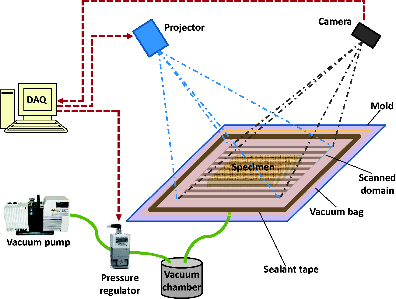

Using a digital vacuum pressure regulator (SMC ITV-2091), a specimen was kept under a compaction pressure, P_c of 80 kPa for 10 min so that the thickness of the specimen reached an almost settled value. Then, P_c was decreased from 80 to 78 kPa almost instantaneously, and h(x,y) was measured after the specimen was kept at this pressure for 30 s. This procedure was continued until the pressure was dropped down to the minimum value, i.e., P_c was 80, 78, 76, … , 4, and 2 kPa.

The results of four repeated compaction characterization experiments for each fabric type are shown in Figure 2. The compaction model constants, C and D in the exponential function given in equation (2) were determined by using least-square method and minimizing the error between the model and the average experimental data.

Figure 2.

Compaction characterization experiments (the error bars show the standard deviation in four repeated experiments for each fabric type) and model fit. Fiber volume fraction, V_f is unitless and P_c is in Pa in the compaction model (see equation (2)).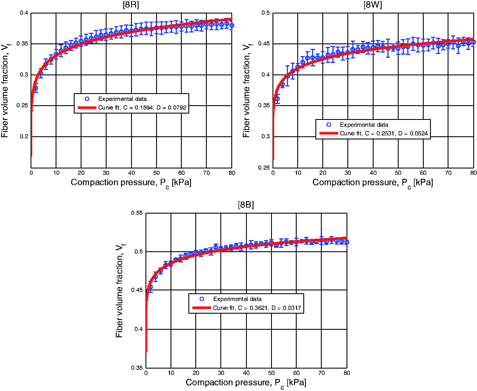

At the maximum compaction level of P_c = 80 kPa, the highest and lowest fiber volume fractions were achieved in [8B] and [8R], as V_f = 51.5 and 38.5%, respectively (see Figure 2). It was also observed that the scatter and thus standard deviation in experimental data was lower in [8B] than in [8R] and [8W], which could be due to the more uniform packing of fiber tows (and thus uniform fiber structures in the specimens) in biaxial fabric than random mat and woven fabric.

Permeability characterization experiments

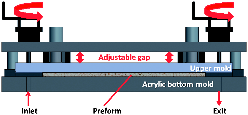
In an earlier study by Yalcinkaya et al.,¹³ sets of one-continuous permeability measurement experiments were conducted at different injection boundary and flow conditions to create a permeability database for the same three fabrics used in this study. The experimental procedure is briefly described here for the completeness of this study; however, the reader is referred to the aforementioned study for details. A mold with adjustable cavity thickness (see Figure 3) was designed and manufactured. The acrylic lower mold plate allowed tracking the flow front propagation to verify if the flow was 1D. Constant-P experiments were conducted by connecting a vacuum pump to the mold at the exit side and a resin reservoir at the inlet. Constant-Q experiments were conducted by connecting a flow-rate-controlled injection machine to the mold at the inlet side. A fabric preform was placed in the mold cavity, the mold was closed and the cavity thickness was set to the initial value. At this initial thickness and thus corresponding V_f, K_unsaturated was measured during mold filling (i.e., transient or also called unsteady flow) by recording and analyzing either the flow front position versus time data for constant-P case or injection pressure versus time data for constant-Q case. After the mold was filled and steady flow condition was obtained, K_saturated at the initial V_f was measured by recording pressure gradient and flow rate. The injection was continued with the initial boundary condition, and K_saturated was measured at different V_f by adjusting the mold gap (thickness, h) and recording the pressure gradient and flow rate for constant-Q and constant-P experiments, respectively.

Figure 3.

The mold used for one-continuous permeability measurement experiments.¹³

The following exponential function was fitted to K versus V_f data

K = {Ae}^{- {BV}_{f}}

(3)

The constants A and B in equation (3) were determined by using least-square method. Four combinations of two injection boundary conditions and two flow conditions resulted in significant differences in permeability constants A and B (see the legends of Figure 4). It was mainly concluded that K measured at constant-Q was higher than the constant-P case (see Figure 4). Also, K_unsaturated was reported to be higher than K_saturated indicating that the test fluid acted as a wetting fluid.⁴⁶ Such differences in permeability measurements under different flow and boundary conditions were also observed in previous studies and they were attributed to dual-scale flow, capillary effect and air bubbles.^13,46,47 During unsaturated in-plane flow in VI and similar processes (i.e., the unsteady transient flow until the resin reaches the exit), microchannels inside fiber tows are impregnated with resin usually later than the impregnation of surrounding empty channels between fiber tows. This is due to much lower intra-tow permeability than the inter-tow permeability. The dual-scale flow causes entrapping of voids (dry regions) behind the flow front which are expected to shrink with time until the surrounding resin pressure and the void pressure equalizes, or the voids are diffused and eventually evacuated from the exit. Some studies modeled the dual-scale flow by adding a sink term to the continuity equation.^48–51 This discussion may convince a reader about why unsaturated and saturated flow experiments yield such differences in permeability data. But, it is not obvious why there is significant difference between the experimental permeability results conducted under constant-Q and constant-P boundary conditions. This may be attributed to different flow regimes in the two experiments. Flow regime is almost constant in the constant-Q experiment, but time-dependent in the constant-P experiment. That means, flow front velocity is almost constant in the constant-Q experiment (unless the effect of dual-scale flow is strong), and it is high initially and decreasing with time in the constant-P experiment.

Figure 4.

Permeability database for three types of fabrics by averaging repeated experimental data; A has a unit of m² and B is non-dimensional (see equation (3)). Note that horizontal V_f domains for the three fabric types differ, and they nearly correspond to these materials’ fiber content when they are compacted during pre-injection vacuuming between 2 and 80 kPa.

1D flow model for VI

This study used 1D flow model for VI process developed by Yalcinkaya and Sozer⁴ in their previous study. Conservation of mass resulted in the following equation after the resin velocity was expressed by using Darcy law

\frac{\partial h}{\partial t} = \frac{1}{μ} \frac{\partial}{\partial x} (Kh \frac{\partial P}{\partial x}) = \frac{1}{μ} (\frac{\partial K}{\partial x} h \frac{\partial P}{\partial x} + K \frac{\partial h}{\partial x} \frac{\partial P}{\partial x} + Kh \frac{\partial 2 P}{\partial x^{2}})

(4)

where h(x,t) is the thickness of the preform, t is time and x is the position along the resin flow. In that study, for typical VI process parameters, it was shown that,

O (\frac{\partial K}{\partial x} h \frac{\partial P}{\partial x}) = O (Kh \frac{\partial 2 P}{\partial x^{2}}) > O (\frac{\partial h}{\partial t})

and

\frac{\partial K}{\partial x} h \frac{\partial P}{\partial x} ≅ - Kh \frac{\partial 2 P}{\partial x^{2}}

, where O(…) represents the order of magnitude. Therefore,

\frac{\partial h}{\partial t}

term in equation (4) was dropped out resulting in the following simplified equation

\frac{\partial}{\partial x} (Kh \frac{\partial P}{\partial x}) = 0

(5)

It is important to notice that although $\frac{\partial h}{\partial t}$ was dropped out, h was allowed to vary with time by using a quasi-steady solution approach (i.e., by solving distributions of P, h and K in the resin-filled domain, and propagating the flow front for the next time step). Also notice that while h and P are related to each other through compaction characterization of the fabric preform, K and h are related to each other through permeability characterization. The simulation results of that study were calculated by numerically solving the 1D flow model for VI (equation (5)) and using K data from unsaturated characterization experiments under constant-P condition (shown with the blue curve in Figure 4). The description of the numerical solution was detailed in that study⁴; however, it will be briefly given here for the completeness of this study. At any instant of mold filling, resin pressure, P is equal to injection and vacuum pressure at the inlet and flow front position, respectively. P distribution between these two ends of the resin-filled region (0 < x < x_f) was solved by using finite difference method and Gauss–Seidel iterative method. The flow front was advanced from x = x_f to x = x_f + Δx by computing the flow front velocity using Darcy law, u_f = −(K_f/(µφ)) ∂P/∂x which took a time step of Δt = Δx/u_f. This numerical procedure was repeated until the flow front arrived at the exit.

Mold-filling experiments

The specimens were vacuum bagged on a flat mold, and mold-filling experiments were conducted under constant pressure differential, ΔP of 80 kPa between inlet reservoir and exit and by using test fluid instead of actual resin as explained earlier (see Figure 5). In Figure 6(a), h(x,y,t = 0) distribution of a dry fabric preform, [8R] is presented to show the spatial variation in h. The mold was placed under the thickness scanning setup so that the thickness distribution of the preform was monitored during the mold filling. The flow front was tracked through the transparent vacuum bag, and arrival times at every 20 mm were recorded.

Figure 5.

Schematic of a mold filling experiment in the VI setup.

Figure 6.

Experimental and simulated evolution of thickness distribution for [8R]. The simulation was run by using constant-P and K_unsaturated permeability characterization. Note that the vertical axis in (c)–(f) is the part thickness normalized by the initial distribution.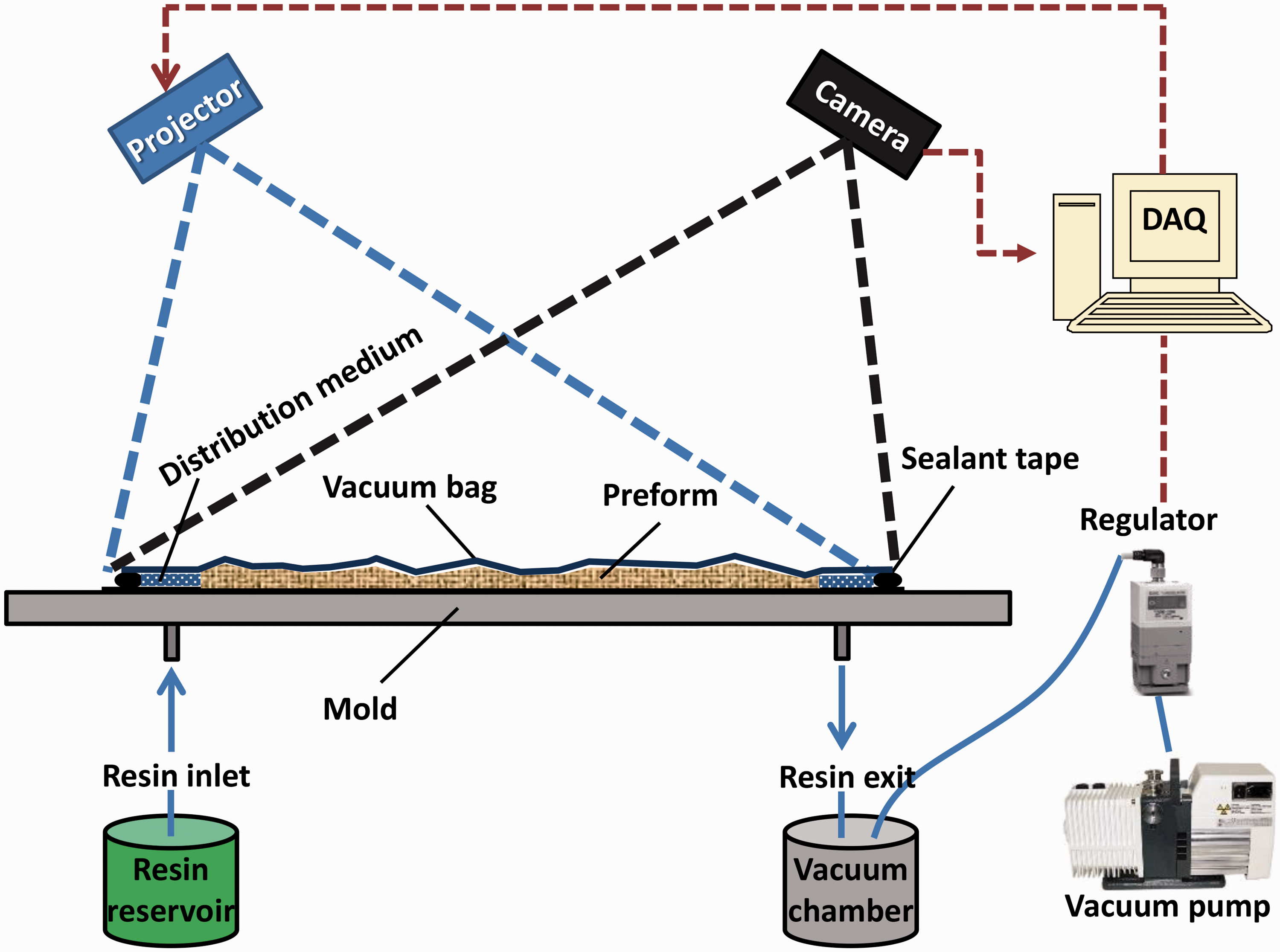

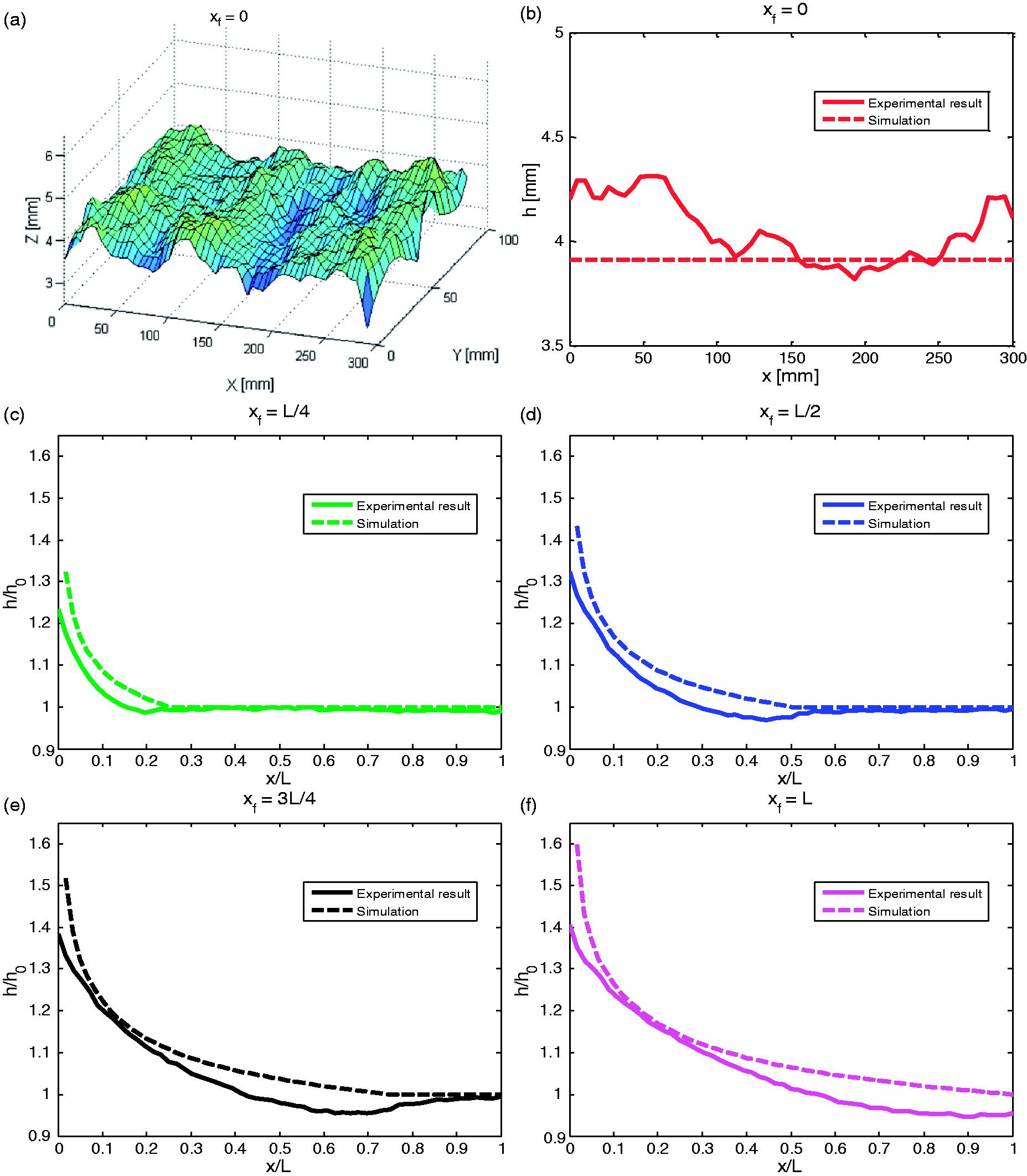
The average thickness distribution of three repeated mold-filling experiments is shown in Figure 6 for [8R] random preform, and later in the next section for all three fabric types studied. The simulation shown in Figure 6 was run by using the result of constant-P and K_unsaturated material characterization. h(x,t) was computed by averaging h(x,y,t) distribution in y direction (see equation (6)). In Figure 6(c)–(f), h(x,t) was normalized by its initial distribution h(x,0) (shown in Figure 6(b)) when the flow front is at x_f = L/4, L/2, 3L/4 and L where L (= 300 mm) is the mold length along the 1D flow direction (see Figure 6). h(x,t) values shown in the graphs are the averaged thickness in y direction, i.e.

h (x, t) \equiv \frac{1}{w} \int_{0}^{w} h (x, y, t) d y

(6)

where w is the width of the specimen in y direction.

Results and discussion

To quantify the effect of using different permeability characterization approaches on the simulated results, coupled 1D resin flow and fiber compaction model for VI were solved by using four different sets of permeability model constants (A and B in equation (3) and tabulated in the legends of Figure 4) corresponding to the combinations of two injection boundary conditions (constant-P and constant-Q) and two flow conditions (unsaturated and saturated). The permeability model constants for the same fabric types used herein were obtained in our previous study.¹³ The compaction model constants (C and D in equation (2) and tabulated in the legends of Figure 2) were determined by running compaction characterization experiments on each fabric type. Mold-filling experiments for all fabric types were conducted and results were compared with the simulations. The experimental flow front position versus time graphs in Figure 7 shows the average of three repeated experiments (blue solid curve) and scatter among these experiments (blue stars). The simulated mold-filling times, t_sim are closest to the experimental data, t_exp (the absolute error, |t_sim−t_exp|/t_exp is 13, 26 and 37% for [8R], [8B] and [8W], respectively) when the permeability characterization is conducted at constant-P boundary condition and the flow is unsaturated. This agrees with the nature of VI mold-filling process in which the injection pressure is constant and the flow is unsaturated. For this recommended permeability testing condition, one may inquire the deviation between the simulated and experimental results, and under-prediction of simulated x_f (t) for the random and biaxial fabric specimens, and over-prediction of it for the woven fabric. These can be attributed to the following three factors ((i)–(iii)). (i) Although both compaction and permeability characterization data from repeated experiments had significant variations, a curve fit was used for each data set (equations (2) and (3), respectively) using least-square method. The simulated results were calculated by using these empirical formulas which represented the mean of the characterization data but not the variation of it. (ii) The model was based on simplification assumptions of elastic compaction behavior, but not viscoelastic, and empirical constitutive equations. (iii) The scatter in the experimental x_f (t) data (see Figure 7) due to non-uniform fiber structure (see Figure 6(a)) and non-repeatable specimen preparation could be larger if the number of repeated VI experiments were increased, and thus the simulated results could be closer to the band of VI results. By considering all of these factors, the accuracy of the aforementioned under- and over-prediction of the simulated x_f (t) may not be definite. However, one can readily conclude that the simulated x_f (t) is consistently closest to the experimental VI data when the permeability characterization is conducted at constant-P boundary condition and the flow is unsaturated.

Figure 7.

Experimental and simulated propagation of flow front with time. Blue stars show each experiment.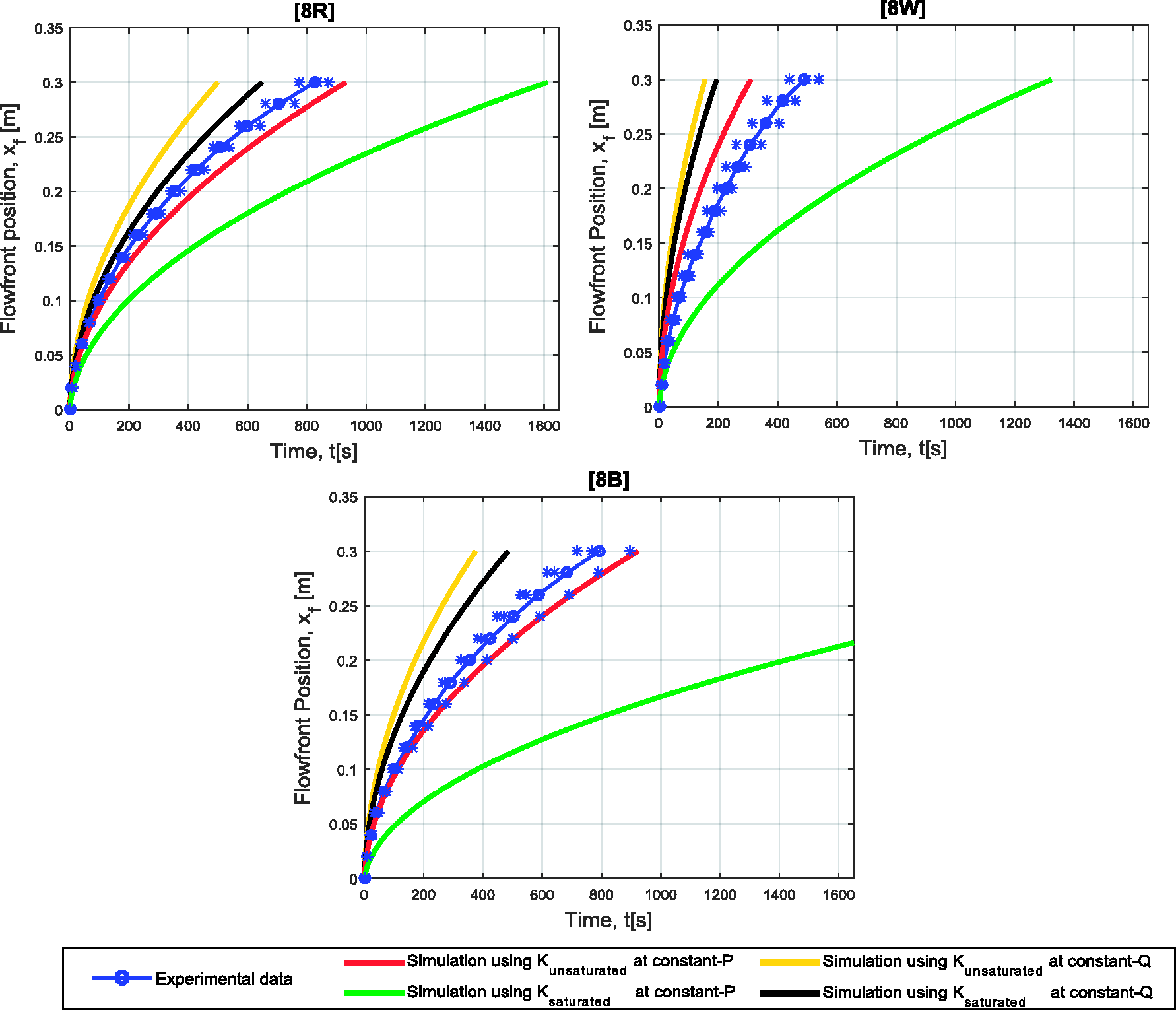

On the other hand, the highest difference between the simulation and experiments (i.e., 95%, 360% and 170% for [8R], [8B] and [8W], respectively) occurs when constant-P and saturated permeability is used. This shows that even though the injection boundary condition in permeability measurement is selected the same as the condition in VI experiments, if the flow type is chosen different (i.e., chosen as saturated instead of unsaturated flow), it leads to enormous error in the mold-filling simulation of VI. Moreover, despite the fact that Darcy law is originally proposed for saturated flows in granular beds, it is commonly used to model the resin flow in LCM that is unsaturated flow during filling stage and saturated flow during post-filling stage.^4,6,7,33 Thus, a modeler should be cautious about the validity of the model as well as how the material characterization is conducted to determine the permeability. A modeler should ideally use K_unsaturated and K_saturated for the filling and post-filling stages in VI, respectively. The injection boundary condition (constant-P or constant-Q) should be selected the same as the actual boundary condition used in the LCM manufacturing process; and it is constant-P type in the VI itself. Therefore, it was expected to see that use of permeability characterization data conducted under unsaturated flow and constant-P boundary condition resulted in the closest simulation to the actual VI experiments. However, use of other possible boundary conditions during permeability characterization was intentionally included in the analysis just to show that a modeler should be cautious when permeability data are taken from an already available database. There are many permeability databases available in the literature which were designed and conducted to model various processes under different flow and boundary conditions. For instance, while it is the most appropriate to use unsaturated permeability under constant-P characterization when modeling VI process, using unsaturated permeability under constant-Q characterization seems the most appropriate when modeling RTM process if a constant-Q resin injection is used. Moreover, unsaturated transverse permeability (K_z) of a fabric preform is also necessary besides in-plane permeability components to simulate mold filling in various processes such as SCRIMP, resin film infusion and compression-RTM since resin flows not only in planar directions but also through-the-thickness (transverse) direction. Thus, the process being modeled should dictate which permeability characterization data are used in simulations for better accuracy.

The evolutions of the simulated thickness distribution for the three fabric preforms along with their corresponding VI experimental data are shown in Figure 8. One observation is that although an elastic compaction model is used here, reasonably close results to experiments are obtained. A modeler can prefer using a viscoelastic compaction model to achieve even better simulated results; however, it comes with the expense of more complicated modeling, tedious material characterization and computational complexity for simulations.

Figure 8.

Comparison of experimental and model results (by using constant-P and K_unsaturated characterization) for the evolution of thickness distribution.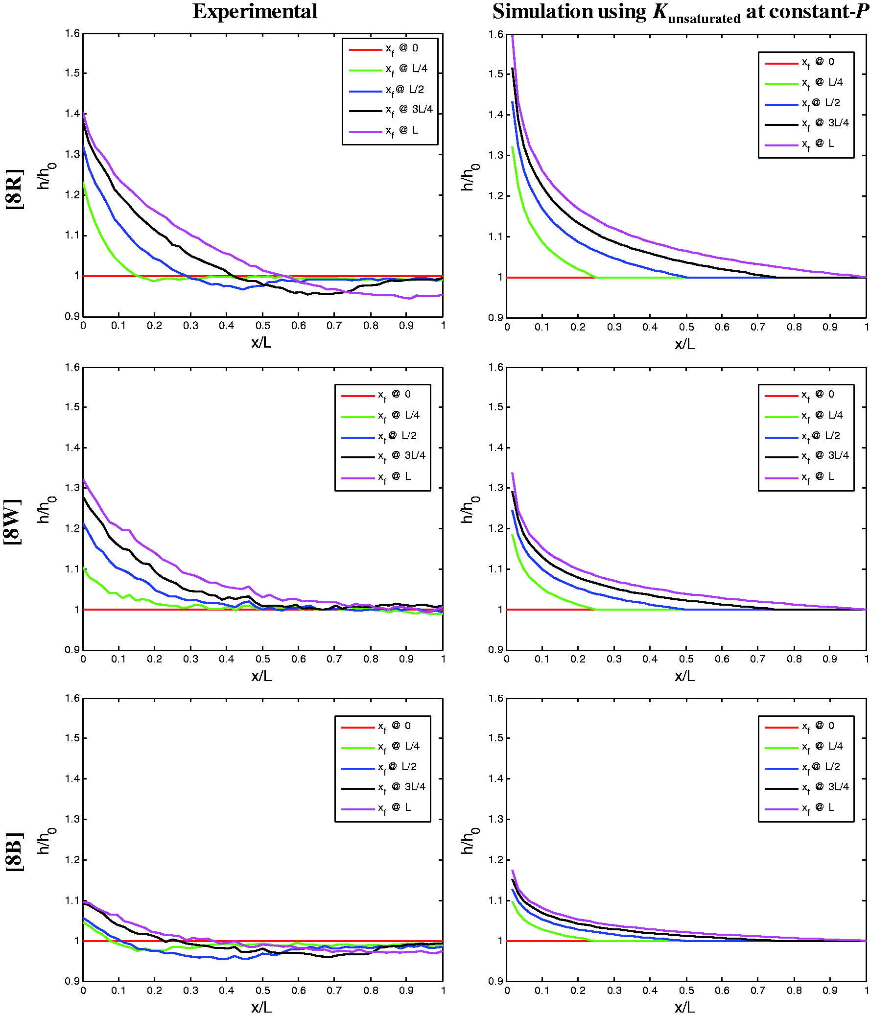

Another observation is that process modeling by using compaction characterization on a dry specimen yields the evolution of thickness distribution fairly close to VI experiments although the fabric is initially dry and becomes wet later during the mold filling in actual VI injections. One should ideally use wet specimens in compaction characterization, or better to start with a dry fabric and saturate it with resin just before the unloading (decompaction) stage as done in the references^5,35,39 to mimic the thinning observed in Figures 6 and 8. There are two reasons for further compaction of a fiber structure observed in VI experiments (see that the normalized thickness gets smaller than one in Figures 6(c)–(f) and 8): (i) lubrication effect at the flow front region after resin arrival, and (ii) dry fiber settling due to viscoelastic behavior which is time-dependent and continues even after the pre-injection vacuuming in dry regions. The former cause is usually the dominant one, and it was observed significantly in previous studies as well^1,41,52 especially for random fabric. This is most probably because of the fact that fiber bundles in a random structure are freer to slide and nested further than in other structures. As seen in Figure 8 and briefly explained earlier, random and biaxial fabrics ([8R] and [8B]) exhibit this phenomenon at and behind the flow front whereas the woven fabric ([8W]) does not exhibit this significantly. The model cannot account for this further thinning near the flow front since the compaction characterization was conducted on dry specimens. If wet specimens are used, or the specimen is wetted between the loading and unloading stages, the compaction characterization resembles the actual VI process better. However, this requires more robust experimental setup and tedious procedure steps as it was done in some previous studies.^1,41 Although the straightforward dry compaction characterization used here did not simulate the further compaction due to lubrication effect for the two fabric types, it modeled fiber decompaction near the inlet reasonably well. Note that h(x,t) increased with time very significantly as the resin pressure increased and compaction pressure decreased (see Figure 6(c)–(f)).

In addition, a modeler should be cautious that the simple compaction model such as the one used here cannot evaluate h and V_f at zero compaction pressure as seen in equation (2). However, except at x = 0, even near the inlet, the thickness distribution calculated by the model and the experiments agree well. Near the inlet, the thickness of the specimen increases rapidly with time due to the fact that higher spring back occurs at low compaction pressures on the material which was also observed in the references.^5,35,39

Conclusion

This study showed that in order to get reasonable results from the simulation of LCM processes like VI, one should use appropriate characterization methods for permeability and compaction of fabrics. Otherwise, the results may deviate significantly from the actual mold-filling results and cause wrong prediction of fill times. The effect of various permeability characterization methods on the mold-filling simulation of VI was investigated for three different types of fabrics. A coupled model was solved numerically to predict the thickness distribution of the fabrics and resin propagation during mold filling. These simulated results were compared with the experimental mold-filling times and thickness distributions of the fabric preforms made of the same three fabric types. It was shown that, permeability data obtained under constant-Pressure injection and unsaturated flow conditions led to the least error in the simulation results compared to the mold-filling experiments whereas constant-Pressure and saturated permeability caused the highest error. Evolution of thickness during mold filling was simulated reasonably well by using a non-linear elastic compaction model. It mimicked the thickening of fabric preforms in resin-filled region as the resin pressure increased with time. However, it was not capable of simulating the thinning near the flow front induced by lubrication effect because the compaction characterization was conducted on dry specimens. Further improvement in modeling of VI can be achieved by (1) using a more complex non-linear viscoelastic compaction model that can demonstrate time-dependent viscous effect and the lubrication effect, and (2) adding a post-filling stage (where the resin flow becomes saturated) thus both K_unsaturated and K_saturated are used for the mold-filling and post-filling stages in VI, respectively.

Footnotes

Declaration of Conflicting Interests

The author(s) declared no potential conflicts of interest with respect to the research, authorship, and/or publication of this article.

Funding

The author(s) received no financial support for the research, authorship, and/or publication of this article.

References

Hammami

. Effect of reinforcement structure on compaction behavior in the vacuum infusion process. Polym Compos 2001; 22: 337–348.

Somashekar

Bickerton

Bhattacharyya

. An experimental investigation of non-elastic deformation of fibrous reinforcements in composites manufacturing. Compos Part A: Appl Sci Manuf 2006; 37: 858–867.

Govignon

Bickerton

Kelly

. Simulation of the reinforcement compaction and resin flow during the complete resin infusion process. Compos Part A: Appl Sci Manuf 2010; 41: 45–57.

Yalcinkaya

Sozer

. Effect of part thickness variation on the mold filling time in vacuum infusion process. J Reinf Plast Compos 2014; 33: 2136–2150.

Yenilmez

Sozer

. Compaction of e-glass fabric preforms in the vacuum infusion process: (a) use of characterization database in a model and (b) experiments. J Compos Mater 2012; 47: 1959–1975.

Correia

Robitaille

Long

. Analysis of the vacuum infusion moulding process: I. analytical formulation. Compos Part A: Appl Sci Manuf 2005; 36: 1645–1656.

Acheson

Simacek

Advani

. The implications of fiber compaction and saturation on fully coupled VARTM simulation. Compos Part A: Appl Sci Manuf 2004; 35: 159–169.

Bayldon

Daniel

. Flow modeling of the VARTM process including progressive saturation effects. Compos Part A: Appl Sci Manuf 2009; 40: 1044–1052.

Caglar

Yenilmez

Sozer

. Modeling of post-filling stage in vacuum infusion using compaction characterization. J Compos Mater 2015; 49: 1947–1960.

10.

Kelly

Umer

Bickerton

. Viscoelastic response of dry and wet fibrous materials during infusion processes. Compos Part A: Appl Sci Manuf 2006; 37: 868–873.

11.

Bickerton

Buntain

Somashekar

. The viscoelastic compression behavior of liquid composite molding preforms. Compos Part A: Appl Sci Manuf 2003; 34: 431–444.

12.

Robitaille

Gauvin

. Compaction of textile reinforcements for composites manufacturing. I: Review of experimental results. Polym Compos 1998; 19: 198–216.

13.

Yalcinkaya

Sarioglu

Sozer

. A novel mold design for continuous permeability measurement of fiber preforms. J Reinf Plast Compos 2015; 34: 915–930.

14.

Sharma

Siginer

. Permeability measurement methods in porous media of fiber reinforced composites. Appl Mech Rev 2010; 63: 1–19.

15.

Gebart

Lidstrom

. Measurement of in-plane permeability of anisotropic fiber reinforcements. Polym Compos 1996; 17: 43–51.

16.

Lundström

Stenberg

Bergström

. In-plane permeability measurements: a nordic round-robin study. Compos Part A: Appl Sci Manuf 2000; 31: 29–43.

17.

Lawrence

Barr

Karmakar

. Characterization of preform permeability in the presence of race tracking. Compos Part A: Appl Sci Manuf 2004; 35: 1393–1405.

18.

Pomeroy

Grove

Summerscales

. Measurement of permeability of continuous filament mat glass–fibre reinforcements by saturated radial airflow. Compos Part A: Appl Sci Manuf 2007; 38: 1439–1443.

19.

Shojaei

Trochu

Ghaffarian

. An experimental study of saturated and unsaturated permeabilities in resin transfer molding based on unidirectional flow measurements. J Reinf Plast Compos 2004; 23: 1515–1536.

20.

Olivero

Hamidi

Aktas

. Effect of preform thickness and volume fraction on injection pressure and mechanical properties of resin transfer molded composites. J Compos Mater 2004; 38: 937–957.

21.

Sozer EM, Chen B, Graham PJ, et al. Characterization and prediction of compaction force and preform permeability of woven fabrics during the resin transfer molding process. In: Proceedings of the fifth international conference on flow processes in composite materials, Plymouth, 1999, pp. 25–36.

22.

Stadtfeld

Erninger

Bickerton

. An experimental method to continuously measure permeability of fiber preforms as a function of fiber volume fraction. J Reinf Plast Compos 2002; 21: 879–899.

23.

Liu

Parnas

Giffard

. New set-up for in-plane permeability measurement. Compos Part A: Appl Sci Manuf 2007; 41: 954–962.

24.

Grossing

Fauster

Weninger

. Influence of textile parameters on the in-plane permeability characteristics of non-crimped fabric preforms. Polym Compos 2016; 37: 1854–1863.

25.

Morren

Bossuyt

Sol

. 2D permeability tensor identification of fibrous reinforcements for RTM using an inverse method. Compos Part A: Appl Sci Manuf 2008; 39: 1530–1536.

26.

Vernet

Ruiz

Advani

. Experimental determination of the permeability of engineering textiles: benchmark II. Compos Part A: Appl Sci Manuf 2014; 61: 172–184.

27.

Arbter

Beraud

Binetruy

. Experimental determination of the permeability of textiles: a benchmark exercise. Compos Part A: Appl Sci Manuf 2011; 42: 1157–1168.

28.

Sun

Lee

. Mold filling analysis in vacuum-assisted resin transfer molding. Part I: SCRIMP based on a high-permeable medium. Polym Compos 1998; 19: 807–817.

29.

Mathur

Heider

Hoffmann

. Flow front measurements and model validation in the vacuum assisted resin transfer molding process. Polym Compos 2001; 22: 477–490.

30.

Chen

Dong

Liang

. Flow modeling and simulation for vacuum assisted resin transfer molding process with the equivalent permeability method. Polym Compos 2004; 25: 146–164.

31.

Hsiao

K-T

Mathur

Advani

. A closed form solution for flow during the vacuum assisted resin transfer molding process. J Manuf Sci Eng 2000; 122: 463–475.

32.

Correia

Robitaille

Long

. Use of resin transfer molding simulation to predict flow, saturation, and compaction in the VARTM process. J Fluids Eng 2004; 126: 210–215.

33.

Hammami

Gebart

. Analysis of the vacuum infusion molding process. Polym Compos 2000; 21: 28–40.

34.

Kang

Lee

Hahn

. Analysis of vacuum bag resin transfer molding process. Compos Part A: Appl Sci Manuf 2001; 32: 1553–1560.

35.

Yenilmez

Senan

Sozer

. Variation of part thickness and compaction pressure in vacuum infusion process. Compos Sci Technol 2009; 69: 1710–1719.

36.

Okonkwo

Simacek

Advani

. Characterization of 3D fiber preform permeability tensor in radial flow using an inverse algorithm based on sensors and simulation. Compos Part A: Appl Sci Manuf 2011; 42: 1283–1292.

37.

Nedanov

Advani

. A method to determine 3D permeability of fibrous reinforcements. J Compos Mater 2002; 36: 241–241.

38.

Yenilmez

Akyol

Caglar

. Minimizing thickness variation in the vacuum infusion (VI) process. Adv Compos Lett 2011; 20: 157–168.

39.

Krehl

Gillespie

. Process and performance evaluation of the vacuum-assisted process. J Compos Mater 2004; 38: 1803–1814.

40.

Yang

Xiao

Zeng

. Compaction behavior and part thickness variation in vacuum infusion molding process. Appl Compos Mater 2012; 19: 443–458.

41.

Yenilmez

Sozer

. Compaction of e-glass fabric preforms in the vacuum infusion process, A: characterization experiments. Compos Part A: Appl Sci Manuf 2009; 40: 499–510.

42.

Tackitt

Walsh

. Experimental study of thickness gradient formation in the VARTM process. Mater Manuf Process 2005; 20: 607–627.

43.

Parnas

Walsh

. Vacuum-assisted resin transfer molding model. Polym Compos 2005; 26: 477–485.

44.

Hubert

Poursartip

. Method for the direct measurement of the fibre bed compaction curve of composite prepregs. Compos Part A: Appl Sci Manuf 2001; 32: 179–187.

45.

Zhang

. Recent progresses on real-time 3D shape measurement using digital fringe projection techniques. Opt Lasers Eng 2010; 48: 149–158.

46.

Michaud

. A review of non-saturated resin flow in liquid composite moulding processes. Transp Porous Media 2016; 115: 581–581.

47.

Diallo L, Gauvin R and Trochu F. Key factors affecting the permeability measurement in continuous fiber reinforcements. In: Proceedings of ICCM-11, Gold Coast, QLD, Australia, 14–18 July 1997.

48.

Binétruy

Hilaire

Pabiot

. The interactions between flows occurring inside and outside fabric tows during rtm. Compos Sci Technol 1997; 57: 587–596.

49.

Patel

Rohatgi

Lee

. Micro scale flow behavior and void formation mechanism during impregnation through a unidirectional stitched fiberglass mat. Polym Eng Sci 1995; 35: 837–851.

50.

Phelan

Leung

Parnas

. Modeling of microscale flow in unidirectional fibrous porous media. J Thermoplast Compos Mater 1994; 7: 208–218.

51.

Amico

Lekakou

. Mathematical modelling of capillary micro-flow through woven fabrics. Compos Part A: Appl Sci Manuf 2000; 31: 1331–1344.

52.

Williams

Grove

Summerscales

. The compression response of fibre-reinforced plastic plates during manufacture by the resin infusion under flexible tooling method. Compos Part A: Appl Sci Manuf 1998; 29: 111–114.