Automated detection and quantification of transverse cracks on woven composites

Abstract

Various loading conditions—cyclic, quasi-static, and dynamic—can induce transverse matrix cracks in cross-ply and woven composite structures. Identification and quantification of this damage on a composite’s surface can provide valuable information on the overall damage state of the structure. This work seeks to develop automated methods for identifying and quantifying transverse matrix crack damage on the surface of composites. To this end, model plain weave glass–epoxy composite specimens were developed that were consistent in geometry and manufacturing process and for which the loading conditions and resulting damage quantity and damage mode could be controlled. High-resolution images (80 megapixel) were captured of the model composite specimen surfaces. These images were then subjected to a manual transverse crack identification method, which established a control with known quantity and spatial location of transverse cracks. Two automated methods were developed to identify and quantify transverse cracks. The first used 8-bit (256 shades of gray) images, an ImageJ preprocessing step, and finally used MATLAB to identify the damage. The second used 16-bit (65,536 shades of gray) images processed directly by MATLAB (no ImageJ preprocessing) to identify the damage. It was found that the 8-bit method more accurately assessed the quantity of transverse cracks because the preprocessing step reduced error-causing high-contrast artifacts (e.g., reflections, composite material inconsistencies, dirt, and ink/marks). Finally, binned scatterplot maps indicating damage quantity and spatial location were created to provide at-a-glance assessment of composite damage condition.

Keywords

Nondestructive evaluation transverse crack damage quantification composite structures image-based crack detection

Introduction

Composite structures are often composed of matrix-infused layered plies or woven yarns of orthogonally oriented fibers. Fiber-direction tensile loading of cross-ply laminates and woven fabric composites induces tensile strain in the transverse plies or yarns and leads to transverse matrix cracking.^1–3 Residual stress from processing and damage from mishandling may also cause transverse matrix cracks. Appearance of transverse cracks on a composite’s surface is an early indicator of structural degradation and damage. Transverse matrix cracking both reduces mechanical properties and leads to fiber fracture clustering and delamination.⁴ The capability to nondestructively identify and quantify matrix cracks on in-service composite structural components is beneficial to the reliability and performance of composites.⁵

Nondestructive techniques for identifying and quantifying transverse cracks include embedded sensors,^6,7 acoustic emission,^8,9 ultrasonic techniques,^10,11 and X-ray,^12,13 but these techniques cannot quantify crack density and are challenging and expensive to apply to in-service vehicles or components.¹⁴ Microscale X-ray computed tomography (μCT) provides high-resolution, three-dimensional, nondestructive visualization of cracking in composites, but it is limited to sample size.¹⁵ In contrast, optical techniques are limited to a two-dimensional surface representation, but are capable of evaluating much larger areas in situ. Automatic, image-based crack detection has been investigated as a replacement for manual crack identification on structural concrete surfaces.¹⁶ Similarly, automatic crack detection has been investigated as a method for quantifying and visualizing transverse cracks in woven composites.¹⁷

An automated, image-based method for detecting and quantifying transverse matrix cracks in composites is useful for postinspection after any type of loading that produces transverse cracks. Transverse cracks are known to occur during quasi-static fatigue loading.¹⁸ Transverse cracks occurring during quasi-static loading of cross-ply laminates have been measured, and models have been developed to predict crack density.¹⁹ Transverse matrix cracking was also found to be a common damage mode in impact of woven composites.^3,17 This dynamic, impact-induced transverse cracking is due to tensile loading of primary yarns under the impactor and in-plane shear transfer of this load into secondary yarns.²⁰ A similar quasi-static mechanism is found wherein punch-shear loading induces transverse matrix cracking.^21,22

Previous efforts to evaluate automated methods for quantifying and visualizing transverse cracks in woven composites used ballistically impacted S-2 glass, SC-15 epoxy composite specimens with a region of interest (ROI) of 8 × 8 in² (203 × 203 mm²).³ These impacted specimens exhibited several damage modes including transverse matrix cracks, 45° matrix cracks, and tow–tow delamination. These damage modes are shown in Figure 1. The six specimens were impacted at velocities ranging from 166 m/s to 439 m/s.²³ The wide range of impact velocities resulted in a large variation in quantities of all damage types. This previous work began with a baseline method in which high-resolution images of the ROI were examined, subdivided into 40 × 40 unit cells, and the cracks in each unit cell were manually counted. These manual counts were then compared to an automated method that used ImageJ²⁴ and MATLAB (The MathWorks, Inc.) to process the images and extract the data.²³ A third method was investigated using fluorophore dyes to illuminate cracks, but it required destructively reducing specimen size to an ROI of 2 × 2.4 in² (50 × 60 cm²) to fit into a fluorescence imager as well as a series of washes to remove excess fluorophore to achieve optimal crack detection. Hence, a nondestructive study comparing specimens of equal size and similar amounts of a single damage mode was needed to further develop and evaluate the performance of automated methods for identifying and quantifying transverse cracks. Therefore, model specimens were developed that were consistent in geometry and manufacturing and for which the loading conditions, and resulting damage quantity, and modes could be controlled.

Figure 1.

(a) Confocal micrographs (left) and back-lit, high-resolution surface images of damage modes (transverse matrix cracks, 45° matrix cracks, and tow–tow delamination cracks) in a woven glass fiber–epoxy composite subjected to dynamic impact. (b) Schematic of how these three damage modes relate in a three-dimensional unit cell of a woven fabric composite.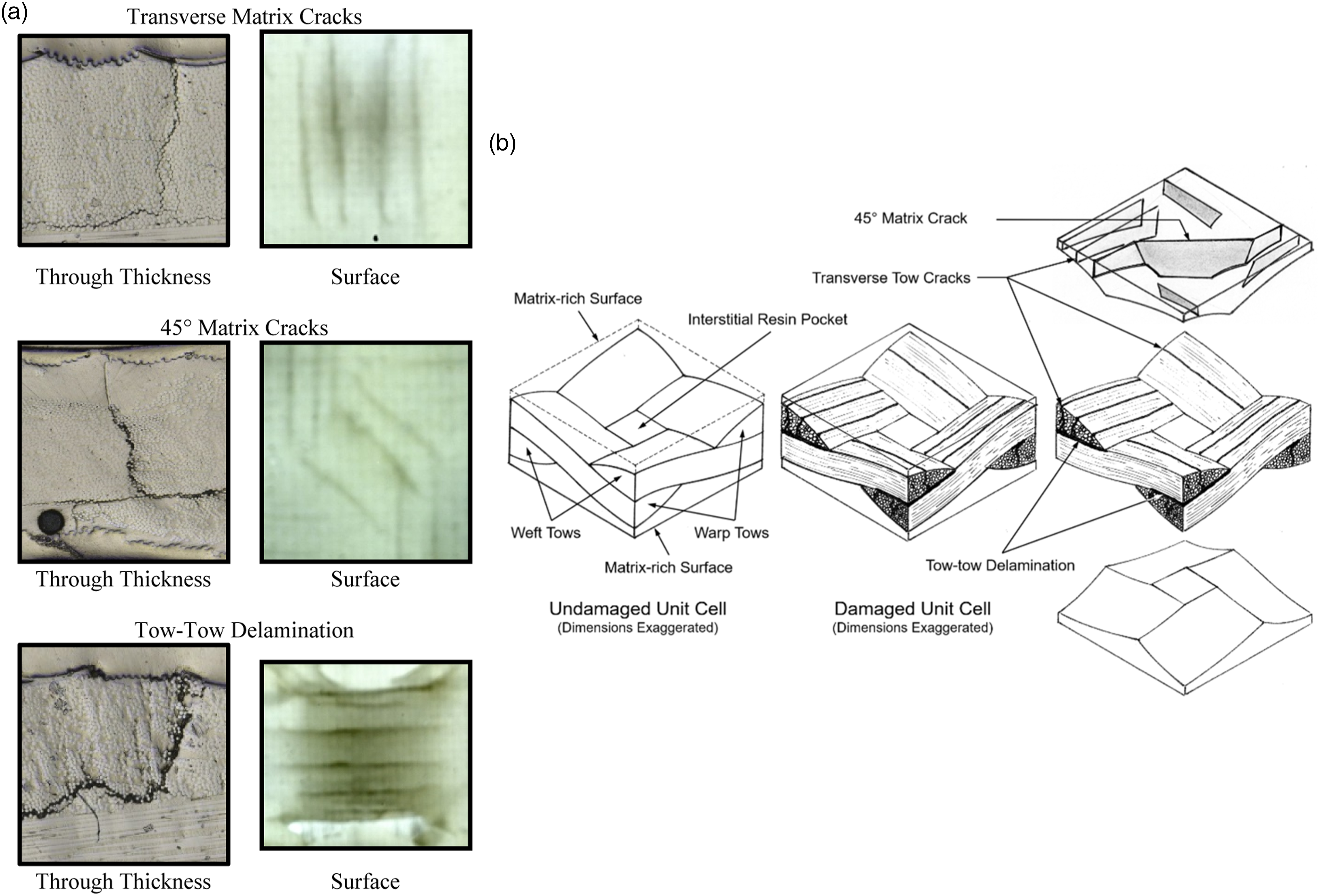

Quasi-static punch-shear testing (described in the next section) was conducted at two load levels to produce consistent results at two damage levels. Dynamic effects, such as transverse deformation cone wave propagation, lead to 45° matrix cracks. Hence, using a quasi-static test method eliminates the presence of these cracks, which are optically similar to transverse cracks but are oriented 45° from transverse cracks. The low energy of the experiments resulted in the presence of minimal tow–tow delamination, and because such delamination cracks propagate parallel to the inspection plane (as seen in Figure 1), they are optically different than transverse cracks and so do not interfere with transverse crack detection.

Specimens were put through two damage identification, quantification, and visualization processes to evaluate these processes relative to a control. The control involved software-enhanced manual counting of the transverse cracks, which is an improvement upon previous work without the software. Additionally, prior work investigated using an 8-bit image processing technique, so a natural extension investigated in the present work is the use of a 16-bit image processing technique. An 8-bit grayscale image includes 256 shades of gray, but a 16-bit grayscale image includes 65,536 shades of gray, so 16-bit images ostensibly include more information. However, the 16-bit images are roughly double the size of 8-bit images, so there is a data-storage cost to using greater bit depth. In this work, the automated 8-bit and 16-bit methods were applied to six specimens at each load level, and the resulting damage identification and quantification was compared with the control results. The techniques and results are described below.

Experiment

Materials

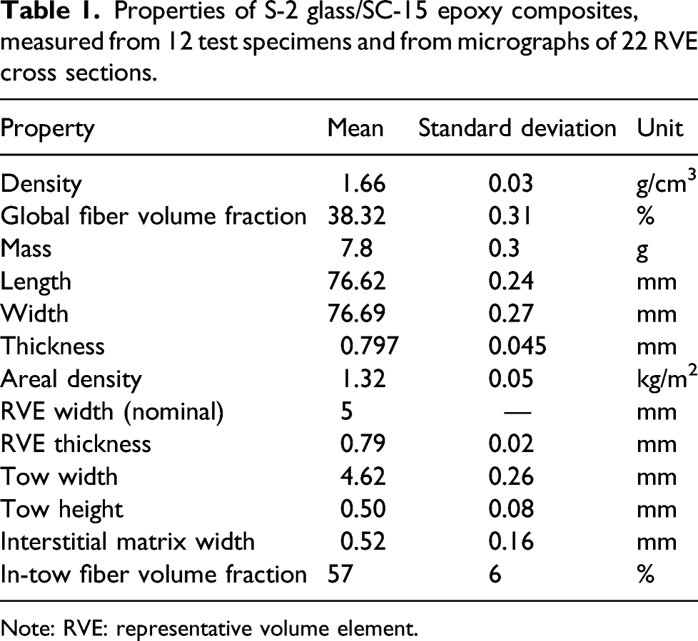
Two 12 × 12 in² (305 × 305 mm²) single-ply composite panels were produced by vacuum-assisted resin transfer molding (VARTM) using plain weave S-2 glass fabric (5 × 5 tows/inch, areal density 744 g/m² (24 oz./yd²), AGY 463-AA-2BL, 30 ends) infused with SC-15 epoxy resin (Kaneka Corp., formerly Applied Poleramic). To ensure uniform surfaces, VARTM was conducted between two glass tooling surfaces as shown schematically in Figure 2(a). Following infusion, shown in Figure 2(b), the composite was cured under vacuum at 35°C (95°F) for 24 h and then the temperature was ramped up at 0.5°C/min to 115°C (239°F) and was held for 3 h. To ensure smooth, undamaged edges, a surface grinder (ACER AGS 1020 AHD) was used to machine 12 test specimens from the two panels: specimens P18-S1 to P18-S9 from panel P18 and specimens P3-S5 to P3-S7 from panel P3. Each specimen was 3 × 3 in² (76 × 76 mm²), which corresponds to 15 × 15 unit cells. A representative test specimen is shown in Figure 2(c). Cross-sectional geometry of a representative volume element (RVE) is shown in Figure 2(d). Properties of the composite are provided in Table 1. Density was measured by pycnometer (ASTM D8171-18) and confirmed by calculation from mass and volume measurements. Global fiber volume fraction (FVF) was measured by burnout (ASTM D3171-99). Global FVF is lower than typical VARTM composites due to the glass tooling, which results in a more resin-rich surface than vacuum bagging alone. This process was used because the controlled surface is more uniform and convenient for finite element modeling. Thickness is averaged from four measurements, one for each of the four specimen ends. Microscopic examination of cross sections (e.g., Figure 2(d)) provided local FVF within tows as well as typical RVE geometry (Table 1).

Figure 2.

Single-ply S-2 glass, SC-15 epoxy composites produced by vacuum-assisted resin transfer molding, (a) shown schematically, and (b) photographically. (c) A representative 3 × 3 in² (76 × 76 mm²) test specimen cut from the single-ply panel before testing. (d) Cross section through orthogonal tows showing internal composite geometry and flat top and bottom surfaces (circular lines are the specimen holder).

Table 1.

Properties of S-2 glass/SC-15 epoxy composites, measured from 12 test specimens and from micrographs of 22 RVE cross sections.

Property	Mean	Standard deviation	Unit
Density	1.66	0.03	g/cm³
Global fiber volume fraction	38.32	0.31	%
Mass	7.8	0.3	g
Length	76.62	0.24	mm
Width	76.69	0.27	mm
Thickness	0.797	0.045	mm
Areal density	1.32	0.05	kg/m²
RVE width (nominal)	5	—	mm
RVE thickness	0.79	0.02	mm
Tow width	4.62	0.26	mm
Tow height	0.50	0.08	mm
Interstitial matrix width	0.52	0.16	mm
In-tow fiber volume fraction	57	6	%

Note: RVE: representative volume element.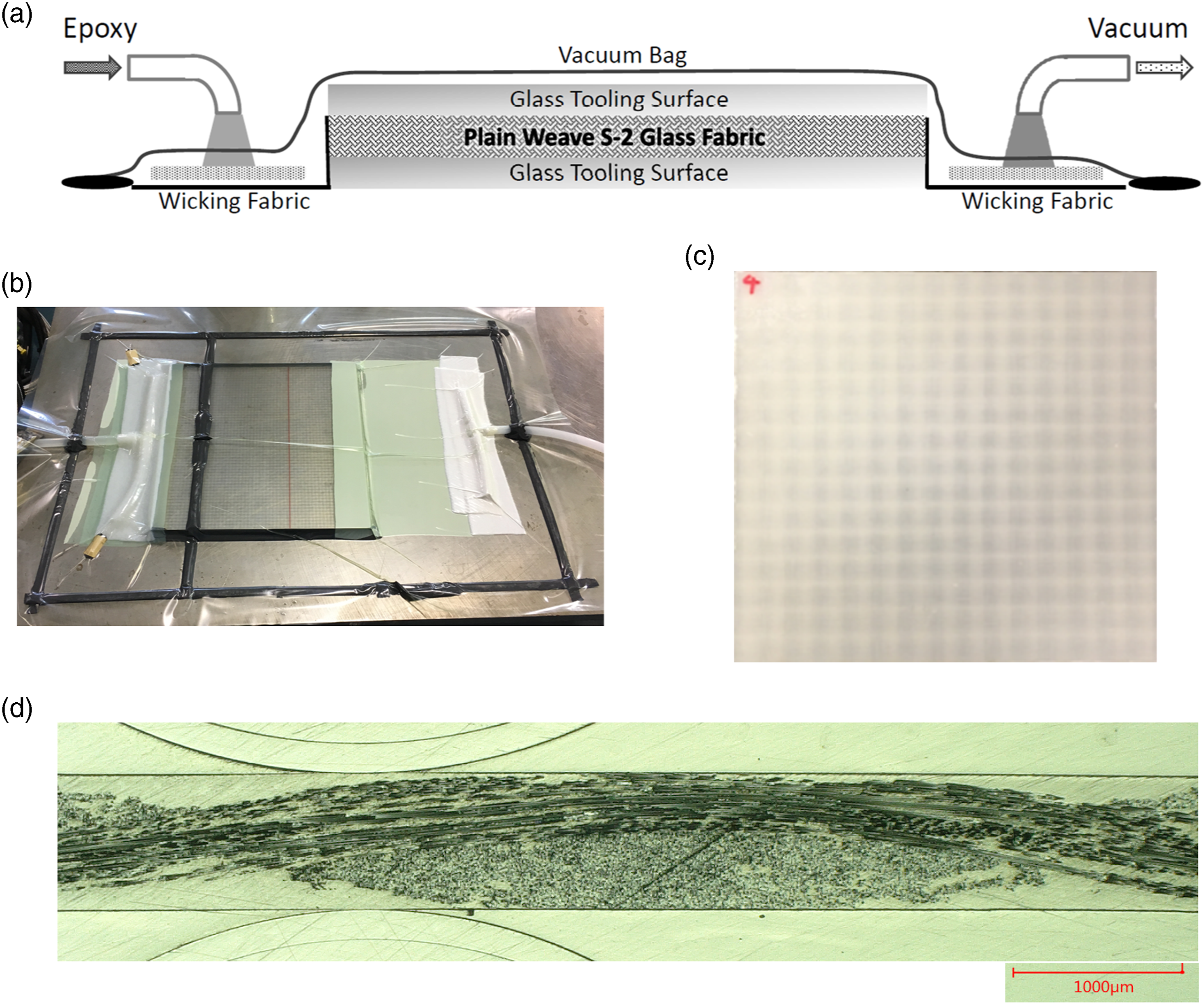

Punch-shear testing

Quasi-static punch-shear testing²¹ was conducted on 3 × 3 in² (76 × 76 mm²) specimens that were clamped in a fixture, shown schematically in Figure 3(a), with $D_{S} = 2 in (50 mm)$ support span. An Instron 5985 load frame with a 30 kN load cell was used to load specimens with a $D_{P} = 0.5 in (12.7 mm)$ hemisphere-nosed punch. As given in Table 1, average specimen thickness is $H_{C} = 0.797 \pm 0.045 mm$ , and each specimen thickness is provided in Table 2. Thickness was measured four times per specimen, once in each quadrant. All tests were conducted at 1.27 mm/min under displacement control. Initially, an experiment was conducted to specimen punch-through failure, which occurred at 2647 N and about 8.5 mm extension. Two load levels were considered, ½ and ⅓ of the maximum (punch-through failure), which corresponded to extensions of about 4.5 mm and 3.0 mm. Tests 1–6, conducted to 4.5 mm extension, resulted in specimens with more damage than tests 7–12, conducted to 3.0 mm extension, and these are subsequently referred to as “½ max” and “⅓ max,” respectively. The average and standard deviation of the area under the curve, which is the total energy of the test at extension, was consistent for each group: 1.426 ± 0.019 N-m (coefficient of variation, COV: 0.013) for ½ max and 0.436 ± 0.029 N-m (COV: 0.066) for ⅓ max. These data are provided in Table 2. Load-displacement curves for tests 1–6 are provided in Figure 3(b). Load-displacement curves for tests 7–12 are provided in Figure 3(c). In this work, damage is only examined on the punch-contact side of the test specimens.

Figure 3.

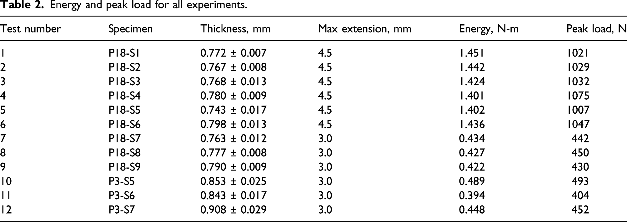
(a) Schematic depiction of punch-shear test fixture with hemispherical punch. Punch is 0.5-inch (12.7 mm) diameter (D_P), support span (D_S) is 2 inches (50.8 mm), and specimen thickness (H_C) is as given above. (b) Load-displacement data for tests 1–6. (c) Load-displacement data for tests 7–12.

Table 2.

Energy and peak load for all experiments.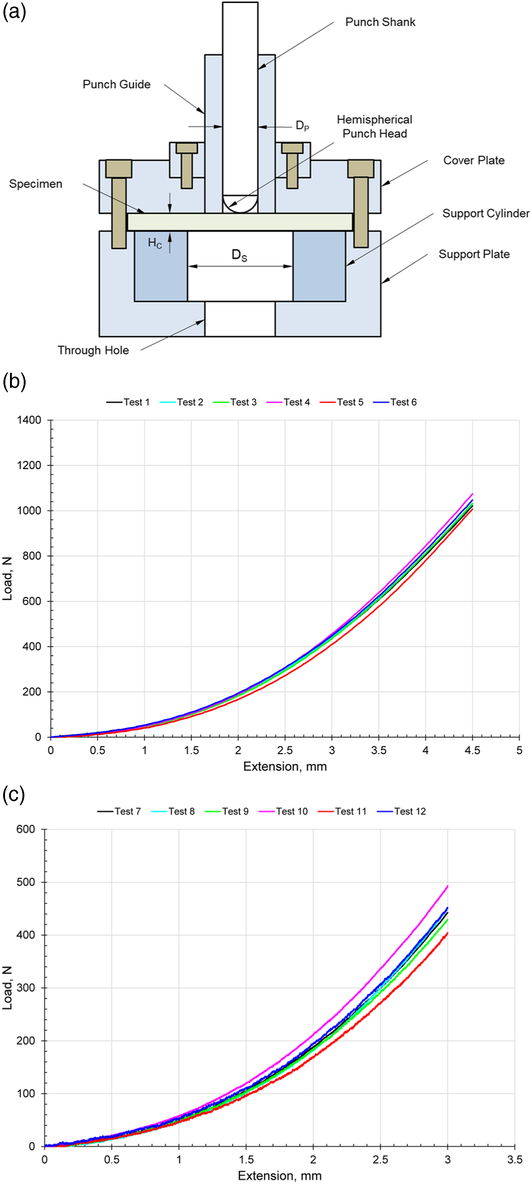

Test number	Specimen	Thickness, mm	Max extension, mm	Energy, N-m	Peak load, N
1	P18-S1	0.772 ± 0.007	4.5	1.451	1021
2	P18-S2	0.767 ± 0.008	4.5	1.442	1029
3	P18-S3	0.768 ± 0.013	4.5	1.424	1032
4	P18-S4	0.780 ± 0.009	4.5	1.401	1075
5	P18-S5	0.743 ± 0.017	4.5	1.402	1007
6	P18-S6	0.798 ± 0.013	4.5	1.436	1047
7	P18-S7	0.763 ± 0.012	3.0	0.434	442
8	P18-S8	0.777 ± 0.008	3.0	0.427	450
9	P18-S9	0.790 ± 0.009	3.0	0.422	430
10	P3-S5	0.853 ± 0.025	3.0	0.489	493
11	P3-S6	0.843 ± 0.017	3.0	0.394	404
12	P3-S7	0.908 ± 0.029	3.0	0.448	452

Specimen characterization and analysis

Post-experimental high-resolution images were captured using a Phase One IQ180 80MP CCD (10,328 × 7760 pixels) digital back and DT-RCam reprographic camera, Phase One 120 mm macro lens, Kaiser RSD adjustable copy stand, and Huion light box backlight and two movable incandescent front lights. 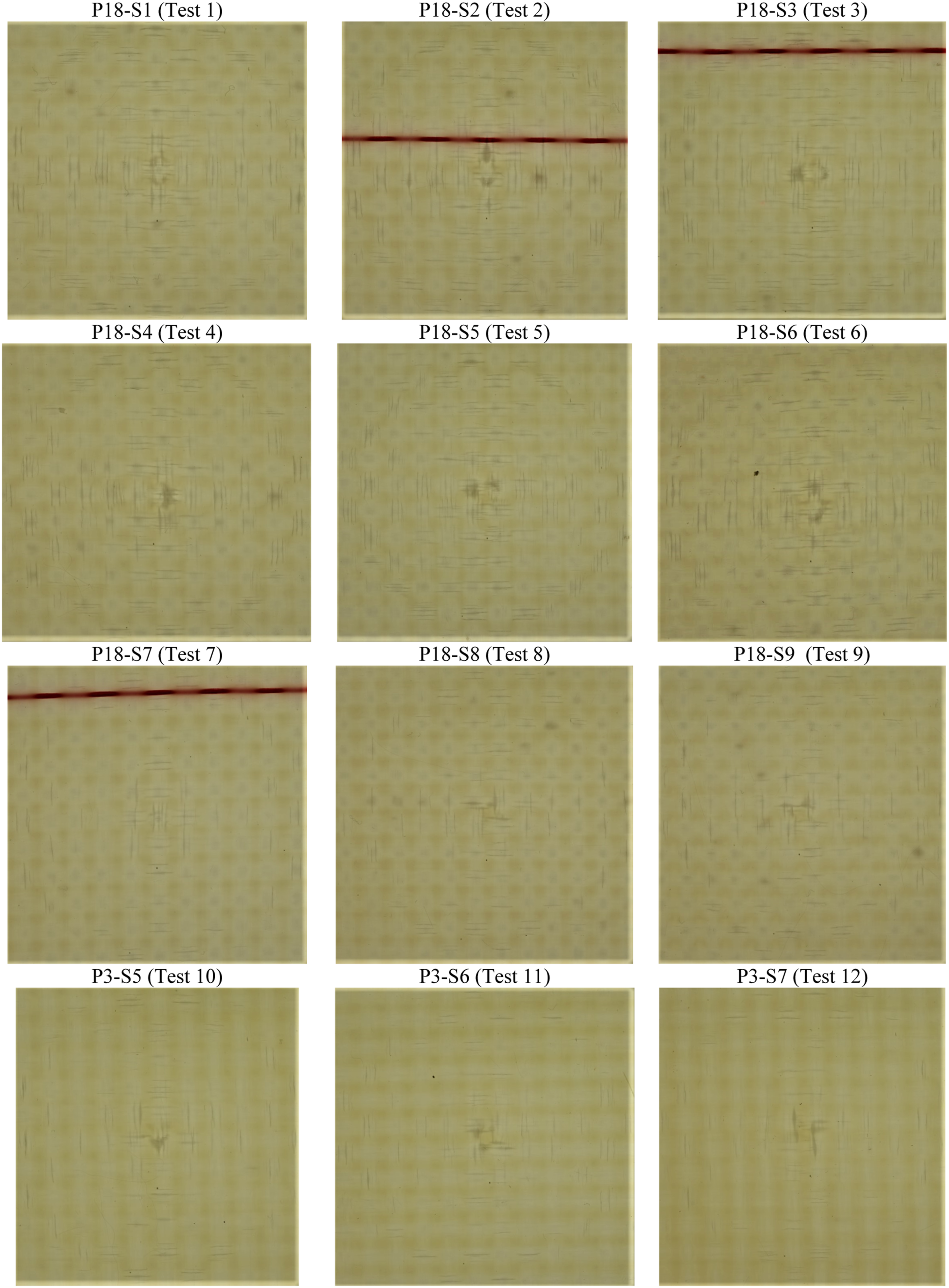Although this work investigated single-layer composites, it may be extended to multilayer composite surface investigations using fluorescence techniques investigated in previous work.²³ Capture One DB 9.1.2 software was used with the Phase One IQ180 to capture RAW images (*.IIQ format). The full resolution of the captured images of the 3 × 3 in² (76 × 76 mm²) specimens is 8205 × 7760 pixels with a spatial resolution of 300 dots per inch. The minimum dimension of image sensor resolution of 7760 pixels means that $76 mm \times 1 pixel / 7760 pixel = 0.01 mm (10 μ m)$ is the smallest sized feature that can be resolved with 1 pixel across. This is sufficient to distinguish multiple transverse cracks across an average $5080 μ m$ tow width (unit cell). Smaller tow widths can also be adequately imaged with current technology, and imaging technology continues to improve, but investigating other tow sizes is beyond the scope of this work. Figure 4 shows that transverse cracks are approximately $10 μ m$ across at the surface, but the projected area of this crack is about $50 μ m$ wide so the difference in contrast between the crack shadow and surrounding uncracked area will have five pixels across. Unprocessed images of the six ½ max and six ⅓ max damaged specimens are provided in Figure 5.

Figure 4.

Confocal micrograph of tow cross section showing transverse crack dimension (fiber diameter $\sim 10 μ m$ ).

Figure 5.

High-resolution images of all damaged S-2 glass/SC-15 epoxy plain weave composite specimens: ½ max load tests 1–6 and ⅓ max load tests 7–12. Full 3×3 in² (76 × 76 mm²) specimens are shown.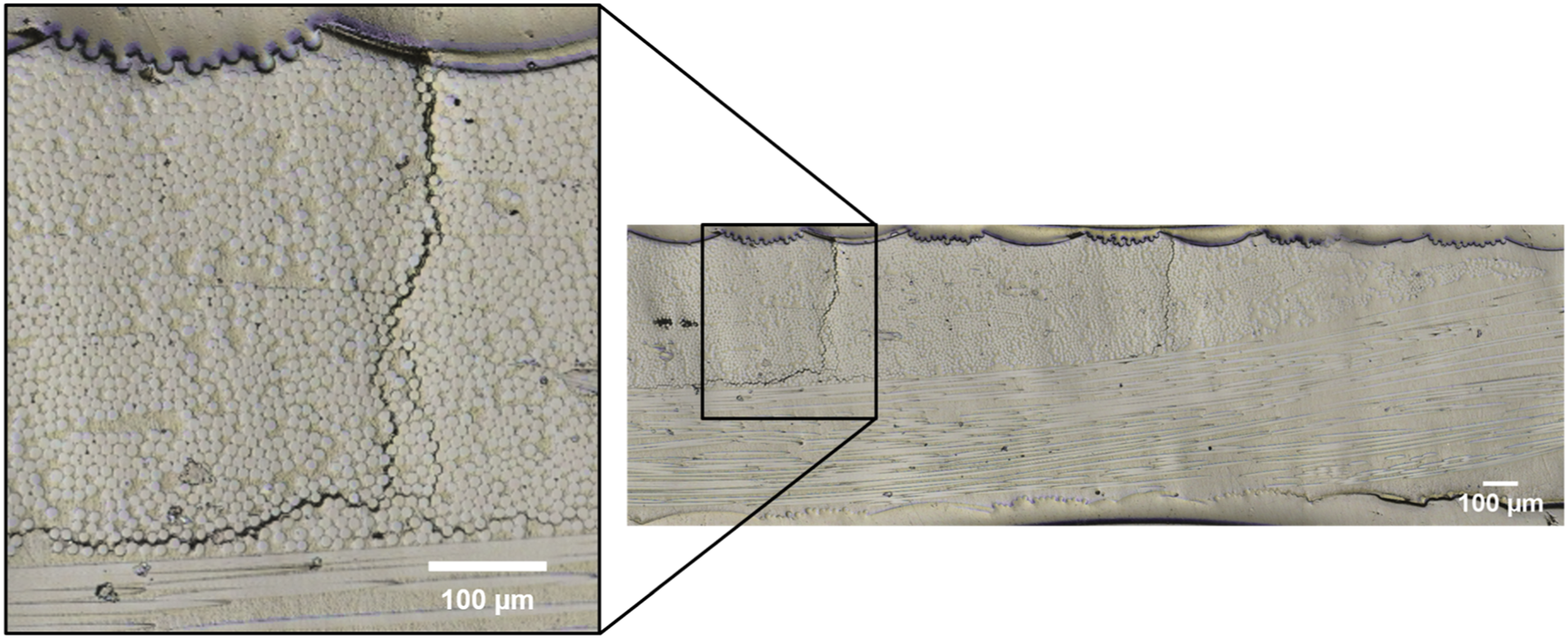

Manual method: Damage counting with LAS X software (a control method)

Raw high-resolution images were converted to JPEG format for fast and efficient manual analysis in commercially available imaging software using a personal computer (PC). Leica Application Suite X (LAS X ver.3.4.2.18368 from Leica Microsystems, Buffalo Grove, IL, USA) software was used on a desktop PC (Intel Core i7-4790, 4-core 8-thread, processor running at 3.6–4.0 GHz and 32 GB of 1600 MHz DDR3 memory). The JPEG images were opened in LAS X, and the transverse cracks were manually traced, measured, and counted on a per-unit-cell basis using the “measure” option in LAS X. Counts of transverse crack damage were saved to a separate Microsoft Excel table (*.XLS format) for each specimen. Damage tables contain 30 columns by 30 rows corresponding to the 3×3 in² (76×76 mm²) specimens, which provide spatial data for the quantified damage. Hence, each column–row pair for each specimen represents half of a unit cell by half of a unit cell. Damage tables were translated into digital damage maps using an in-house written MATLAB (build R2019b) script described previously.¹⁷ The total time required to manually process a single image is approximately 120 min. To minimize human error, manual damage counts were verified by at least two operators. Because of the high confidence in the accuracy of the damage quantification results, this manual method is the control to which subsequent automated methods are compared.

Automated method 1: 8-bit image processing using ImageJ and MATLAB

ImageJ (version 1.52p) was used to trace, analyze, and quantify the transverse crack damage in each of the 12 specimens. Images were loaded into ImageJ software and converted from 16-bit color JPEG into 8-bit grayscale (hence, “8-bit method”). A ridge detection plug-in was then applied to identify horizontal and vertical transverse cracks. For all specimens, the ridge detection plug-in parameters were set as follows: line width = 0.01 μm, minimum and maximum line lengths = 10 μm and 50 μm, low and high contrast = 87, 230, and lower and upper threshold = 2.8 and 7. Count summaries were generated for the transverse crack damage in each specimen. Then 8-bit grayscale images of transverse crack damage were generated for each specimen and exported in JPEG format. Pixels in these images were all in the color range 0–20 (dark) and 220–255 (light), hence straightforward to binarize without error associated with threshold value. “Binarize” means to make an image binary wherein all pixel gray color values above a threshold value are turned to white pixels, and all pixel gray color values below that threshold are turned to black pixels. These images provide transverse crack damage separated from the background.

The processed ImageJ output grayscale images were imported into MATLAB. Images were binarized using the “imbinarize” function in the image processing MATLAB script (MATLAB-1), which uses Otsu’s method for thresholding.²⁵ The “bwboundries” function in MATLAB was then used (“noholes”) to separate the background from objects (damage) to identify cracks. To reduce the risk of including artifacts that were not cracks, a length constraint was applied to the output of the “bwboundries” function. Using a selected specimen (P18-S6), optimization of line intensity for identifying transverse cracks was carried out for line intensities from 1 to 200 pixels using MATLAB-1. For the 8-bit automation method, it was found that a constraint of 130 pixels for line intensity was optimal for identifying horizontal transverse cracks and five pixels for vertical transverse cracks. The output from the line intensity optimization study is included as Figure S1 and Figure S2 in the Supplementary Information. This damage identification process runs separately for horizontal transverse cracks and then for vertical transverse cracks.

In addition, a secondary optimization step was performed for the damage map block size, which corresponds to visualization of damage within specimen unit cell(s). Damage map blocks comprising rows and columns ranging from 15 × 15 px² to 50 × 50 px² were optimized using MATLAB-1. It was found that optimal digital damage maps were generated for horizontal cracks by constraining block size to 35 × 35 px² and for vertical cracks by constraining block size to 5 × 5 px².

Following MATLAB crack identification, the image is broken down into 35 × 35 px² squares, which represents one composite unit cell. Damage within each square is automatically recorded and exported to an Excel file. Excel files are imported into a second MATLAB script (MATLAB-2), which transforms the file into a numeric matrix corresponding to the size of the composite material under consideration. MATLAB-2 then generates a digital damage map for the transverse crack damage, which allows the data to be graphically represented by a grayscale binned scatterplot to visualize the damage data at a glance.

Automated method 2: 16-bit image processing using MATLAB

In this method, high-resolution images in JPEG format were first cropped to 668 pixel x 689 pixel (300 dots per inch, bit depth of 24) with the following adjustments: clarity = 100%, light = −25% using Microsoft Photos software on a PC (Windows operating system 10, build 1903), and saved in 16-bit JPEG format (note that this preprocessing was carried out manually here, but is straightforward to automate using MATLAB or a similar tool). The 16-bit method was optimized similar to the 8-bit method. The optimal line intensity for identifying transverse cracks was identified using MATLAB-1 by examining results for line intensities from 5 to 15 px for a selected specimen (P18-S6). It was found that a constraint of nine pixels for line intensity was optimal for identifying horizontal cracks and five pixels for vertical cracks for the 16-bit automation method. For the 16-bit automation method, output from the optimization of intensity is provided in Figure S3. Optimal digital damage maps were generated for horizontal cracks by constraining block size to 35 × 35 px². Optimal digital damage maps were generated for vertical cracks by constraining block size to 5 × 5 px². To ensure best results, application of these automated methods to specimens from different configurations or test conditions will require optimization of line intensity parameters for each new series. As with the 8-bit automated method, this damage identification process runs first for horizontal and then for vertical transverse cracks.

Cropped high-resolution images were imported into MATLAB-1, the background was separated from damage, and transverse cracks were identified using the optimized line intensity parameters. Following MATLAB crack identification, the image is broken down into 35 × 35 px² squares, each of which represents one composite unit cell. Damage within each square is automatically recorded and exported to an Excel file. Excel files are imported into MATLAB-2, which transforms the file into a numerical matrix corresponding to the size of the composite material under consideration. MATLAB-2 then generates a digital damage map for transverse crack damage, which allows the data to be graphically represented by a grayscale binned scatterplot to visualize the damage data at a glance.

Processing time

A flowchart of the automated methods (both 8-bit method 1 and 16-bit method 2) is provided in Figure 6. The flow chart includes approximate processing time for a single image, to compare the time involved in each of the automated methods. The first step involves capturing high-resolution images (HRIs). Next, for 8-bit processing, the second step is to preprocess the HRI with ImageJ. An example of the output from this preprocessing step, applied to posttest specimen P18-S6, is provided in Figure 6, Step 2. The binary output from ImageJ is shown as black cracks on white background. For 16-bit processing, the second step is the same as step 3 for 8-bit processing, as in Figure 6 (i.e., the 16-bit method does not include ImageJ preprocessing). The MATLAB-1 script is applied to the image (either preprocessed output from ImageJ for 8-bit or HRI for 16-bit) with previously optimized parameters. Sample output from step 3 is provided in Figure 6 where the binary image is shown as white cracks on a black background to differentiate it from the ImageJ step. The tabulated damage output from step 3 (MATLAB-1) is input to MATLAB-2 in step 4, which plots binned scatterplots of the damage. The manual counting method takes about 120 min per sample, the automated 8-bit method takes about 10 min per sample, and the automated 16-bit method takes about 20 min per sample. For the 16-bit automated method, processing time is approximately double that of the 8-bit method because computation time is increased due to the larger image file size and the processing of these images is more complex because they are not imported as preprocessed binary images. The processing time is short for all of these methods compared with CT scanning, for example, and automated processing time may be further reduced using more/faster computer processors.

Figure 6.

Schematic depiction of 8-bit and 16-bit automated damage assessment methods. All images show results from processing specimen P18-S6.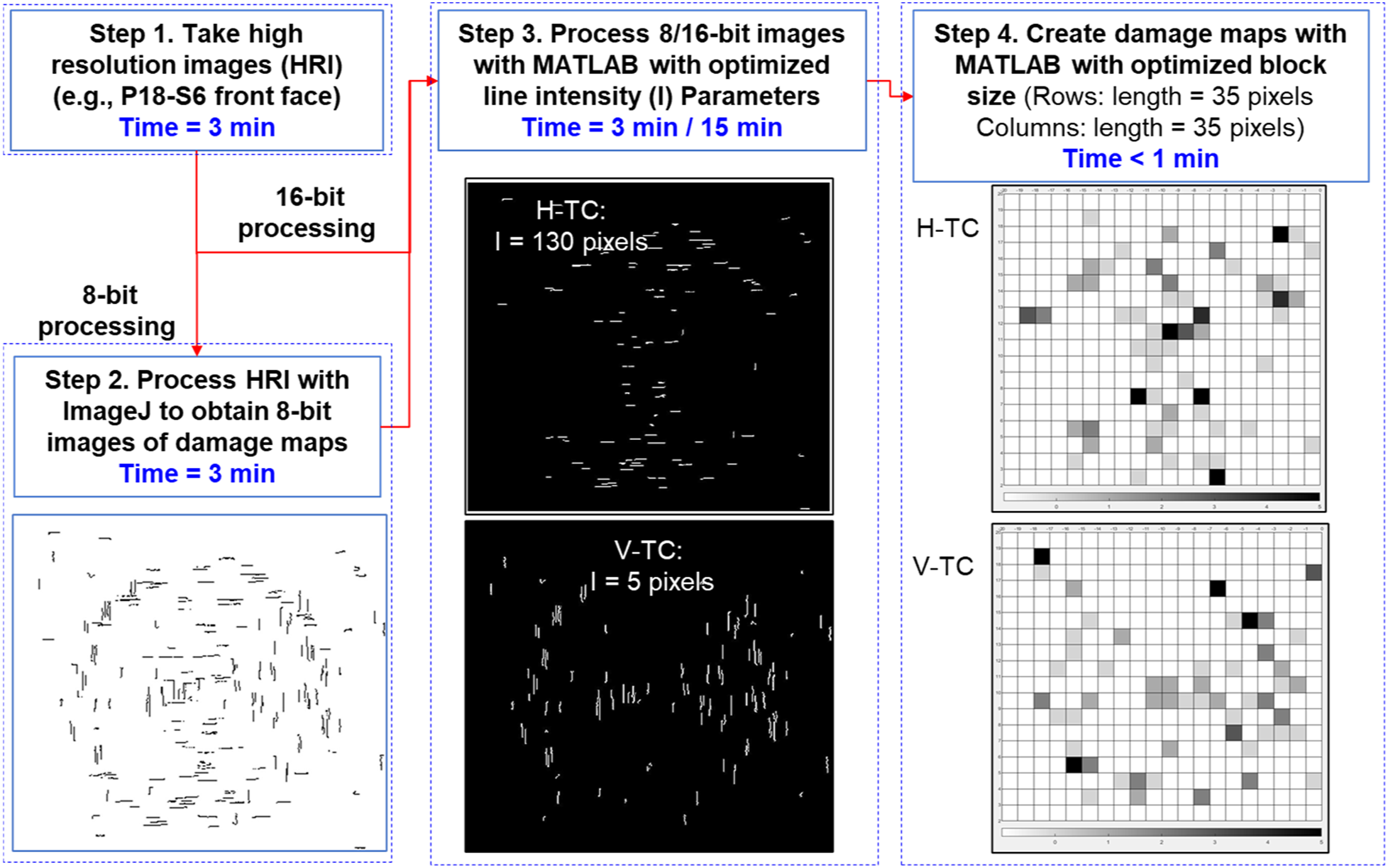

Results and discussion

Manual method (control)

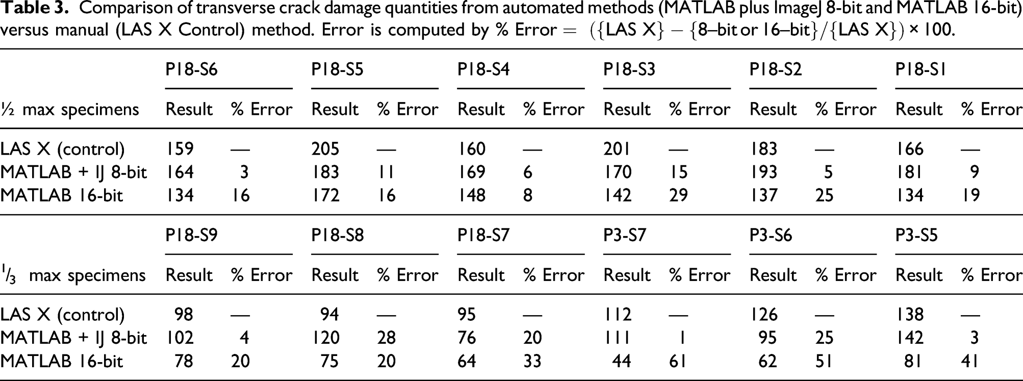
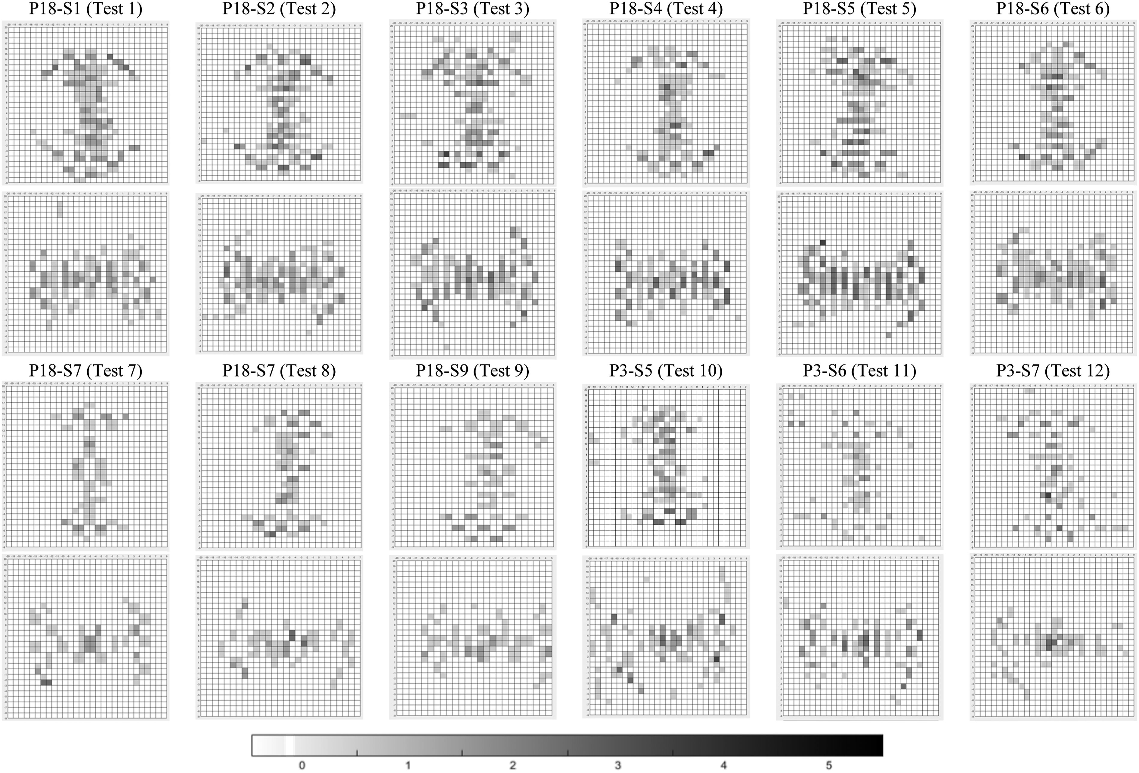
The transverse crack identification results from the manual method, assisted by LAS X software, are provided in Figure 7. The high-resolution images of each specimen are imported into the LAS X software, the images are scaled up so the user can easily identify transverse cracks, and the software is used to manually mark the location and length of each crack. Marked cracks are manually counted, and images of the identified cracks overlaid on the ROI are exported. The results in Figure 7 show each crack marked for both the ½ max and ⅓ max test specimens. The total transverse crack counts found with the LAS X manual method are provided in Table 3 for the ½ max and ⅓ max experiments. It is worth noting that the test fixture and support span used in the experiments result in the specimen being clamped on the region outside the support span, and this means that the majority of transverse cracks will be found within the diameter of the support span. This is exactly what is observed in Figure 7. The damage data tables were plotted as digital damage maps¹⁷ shown in Figure 8. Qualitatively comparing the damage maps in Figure 8 to the experimental results in Figure 7, the concentration of damage within the support span diameter and the severity of damage, as indicated by color (darker means more damage), is captured well by the damage maps. These damage maps provide the operator an at-a-glance view of the damage state of the specimen.

Figure 7.

High-resolution images of ½ max load (tests 1–6) and ⅓ max load (tests 7–12) damaged specimens. Full 3 × 3 in² (76×76 mm²) specimens are shown. Horizontal transverse cracks (top) and vertical transverse cracks (bottom) were manually identified and counted using LAS X imaging software.

Table 3.

Comparison of transverse crack damage quantities from automated methods (MATLAB plus ImageJ 8-bit and MATLAB 16-bit) versus manual (LAS X Control) method. Error is computed by $% Error = ({LAS X} - {8 –bit or 16 –bit} / {LAS X}) \times 100$ .

½ max specimens	P18-S6		P18-S5		P18-S4		P18-S3		P18-S2		P18-S1
½ max specimens	Result	% Error	Result	% Error	Result	% Error	Result	% Error	Result	% Error	Result	% Error
LAS X (control)	159	—	205	—	160	—	201	—	183	—	166	—
MATLAB + IJ 8-bit	164	3	183	11	169	6	170	15	193	5	181	9
MATLAB 16-bit	134	16	172	16	148	8	142	29	137	25	134	19

⅓ max specimens	P18-S9		P18-S8		P18-S7		P3-S7		P3-S6		P3-S5
⅓ max specimens	Result	% Error	Result	% Error	Result	% Error	Result	% Error	Result	% Error	Result	% Error
LAS X (control)	98	—	94	—	95	—	112	—	126	—	138	—
MATLAB + IJ 8-bit	102	4	120	28	76	20	111	1	95	25	142	3
MATLAB 16-bit	78	20	75	20	64	33	44	61	62	51	81	41

Figure 8.

LAS X manual method: damage maps for ½ max load (tests 1–6) and ⅓ max load (tests 7–12) full 3 × 3 in² (76 × 76 mm²) specimens are shown with spatially indicated quantities of horizontal transverse cracks (top) and vertical transverse cracks (bottom). The color bar indicates quantity of cracks.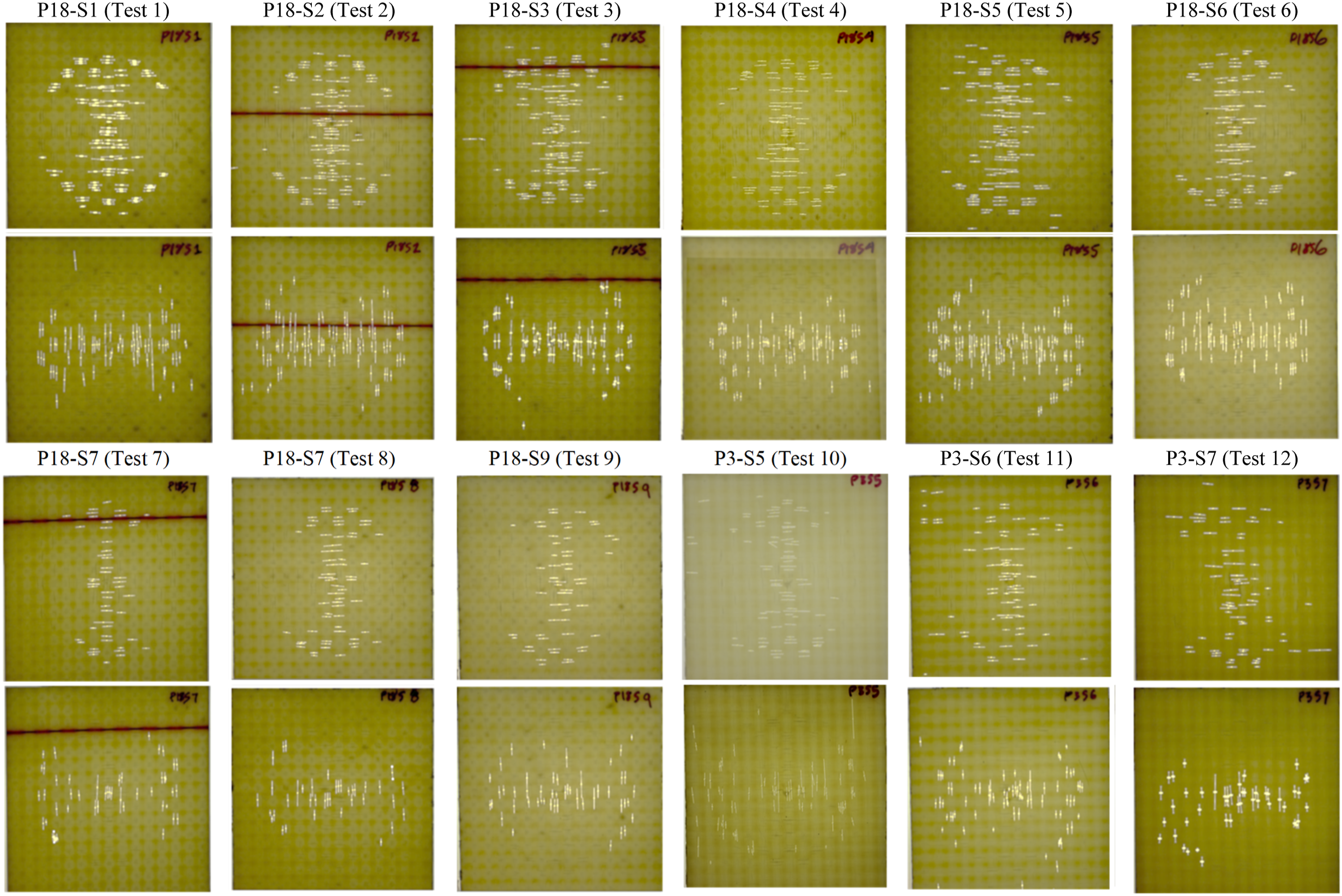

Automated method 1 (8-bit)

For the ½ max and ⅓ max load experiments, transverse crack identification results from the first automated method, which includes an ImageJ preprocessing step, are reported in Table 3. The output from the ImageJ preprocessing step and from the MATLAB step are provided in the Supplementary Information Figure S4 and Figure S5 for ⅓ max and ½ max experiments.

Automated method 2 (16-bit)

For the ½ max and ⅓ max experiments, transverse crack identification results from the second automated method, which directly imports HRI into MATLAB-1, are reported in Table 3 (total crack counts). The output from MATLAB is provided in the Supplementary Information Figure S6 for ⅓ max and ½ max experiments.

Evaluation of the automated methods

From the damage data output by MATLAB-1, total transverse crack counts were found for all specimens using both 8-bit and 16-bit automated methods. These data are compared with the manually counted control results in Table 3. The binary output from ImageJ (8-bit) provided in Figure S4a and Figure S5a may be visually compared to the control results in Figure 7. Qualitative comparison of these results suggests that the ImageJ preprocessing is separating the cracks from the background reasonably well. These data are input into MATLAB-1, processed, and output as white cracks on a black background (to differentiate between ImageJ and MATLAB results). All three methods, 8-bit (Figure S4 and Figure S5), 16-bit (Figure S6), and manual (Figure 7), show the circular region of cracks inside the support span diameter, which is a result of the loading conditions. All three methods also show the typical appearance of transverse cracks confined within alternating unit cells, which is a result of the woven fabric geometry. It appears in the 8-bit results that cracks are shorter or divided since many small cracks appear, and these results are overall less reminiscent of the control than the 16-bit results. In the 16-bit results, while the crack field appears qualitatively very similar to the actual crack field, some noise is present due to light reflections in the images and the red yarn found in some specimens. The processing works by separating the foreground (cracks) from the background, so any high-contrast artifacts (reflections, red yarns, dirt, ink marks, etc.) could be interpreted as cracks. These are not present in the 8-bit images because the ImageJ preprocessing step eliminates them, but also reduces the cracks to lines while the 16-bit method more truly maintains the crack appearance.

For all specimens tested at ½ max load, quantitative results for total crack count are found in Table 3. The LAS X manual count (control) has an average and standard deviation of 179 ± 21 cracks, a 12% coefficient of variation (COV). The 8-bit (automated method 1) average is quite similar to the control, 177 ± 11 cracks, and has a 6% COV. The 16-bit (automated method 2) average of all specimens tested at ½ max load is outside of the experimental scatter (control), 145 ± 15 cracks (10% COV). For all specimens tested at ⅓ max load, the average and standard deviation for the LAS X manual count (control) is 111 ± 18 cracks (16% COV); for the 8-bit method, 108 ± 23 (21% COV); and for the 16-bit method, 67 ± 14 (21% COV). Overall, comparing the percent error included in Table 3, the 8-bit method has greater accuracy than the 16-bit method. As mentioned earlier, the ImageJ preprocessing step reduces the error associated with high-contrast artifacts, so the 8-bit method is more accurate than the 16-bit method, which does not include this step. Additionally, including more data, as in 16-bit images vs. 8-bit images, can also include more high-contrast artifacts. Also, there is more error for the less damaged ⅓ max load than for the more damaged ½ max load. This suggests that the automated methods are better able to find cracks when there are more cracks to find.

It should be noted that there is a difference in experimental results when comparing the LAS X (control) total counts for the ⅓ max load specimens in Table 3. The experiments on samples from Panel 3 show more total damage than the experiments on samples from Panel 18. The data in Table 2 include all specimen thicknesses, and the average thickness of Panel 3 specimens is 0.868 ± 0.039 mm, while the average thickness of Panel 18 specimens is 0.773 ± 0.019 mm. Thickness difference is primarily in the matrix since the fabric is from the same roll, and the difference is due to the greater surface matrix thickness resulting from the glass tooling fabrication method. Length and width of all specimens was similar with a coefficient of variation (standard deviation ÷ average) of less than 0.4% (see Table 1). Thickness affects mass, so average mass and standard deviation are 8.2 ± 0.3 g for Panel 3 and 7.6 ± 0.1 g for Panel 18, and the areal densities are then 1.40 ± 0.05 for Panel 3 and 1.30 ± 0.02 for Panel 18. As seen in Figure 3(b) and in Table 2, the total energy and peak load for the 3.0 mm extension experiments of the Panel 18 (tests 7–9) and Panel 3 (tests 10–12) are similar. The reason for the difference in damage quantity is the greater matrix thickness of Panel 3, which results in formation of more brittle matrix cracks during flexure. However, considering results for Panel 18 alone or Panel 3 alone still arrives at the same conclusion, which is that the 8-bit method is more accurate than the 16-bit method for reasons discussed earlier. Development of a calibration standard could solve the issue of panel-to-panel variation. However, such development leads to other issues such as how to produce real damage while controlling where and how much damage is produced or such as how to produce simulated damage while ensuring damage identification algorithms work for real damage.

Transverse cracks are small and common in a woven fabric composite, and the energy of each crack is minute, so a large number of cracks are expected to be present before the overall structural health of a composite is critically affected. Despite the occasional large error, it is believed that these automated techniques are useful for indicating the overall condition in terms of the presence and quantity of surface transverse cracks. Additionally, in real structural composites, less resin-rich surfaces will increase accuracy with fewer reflected-light optical artifacts.

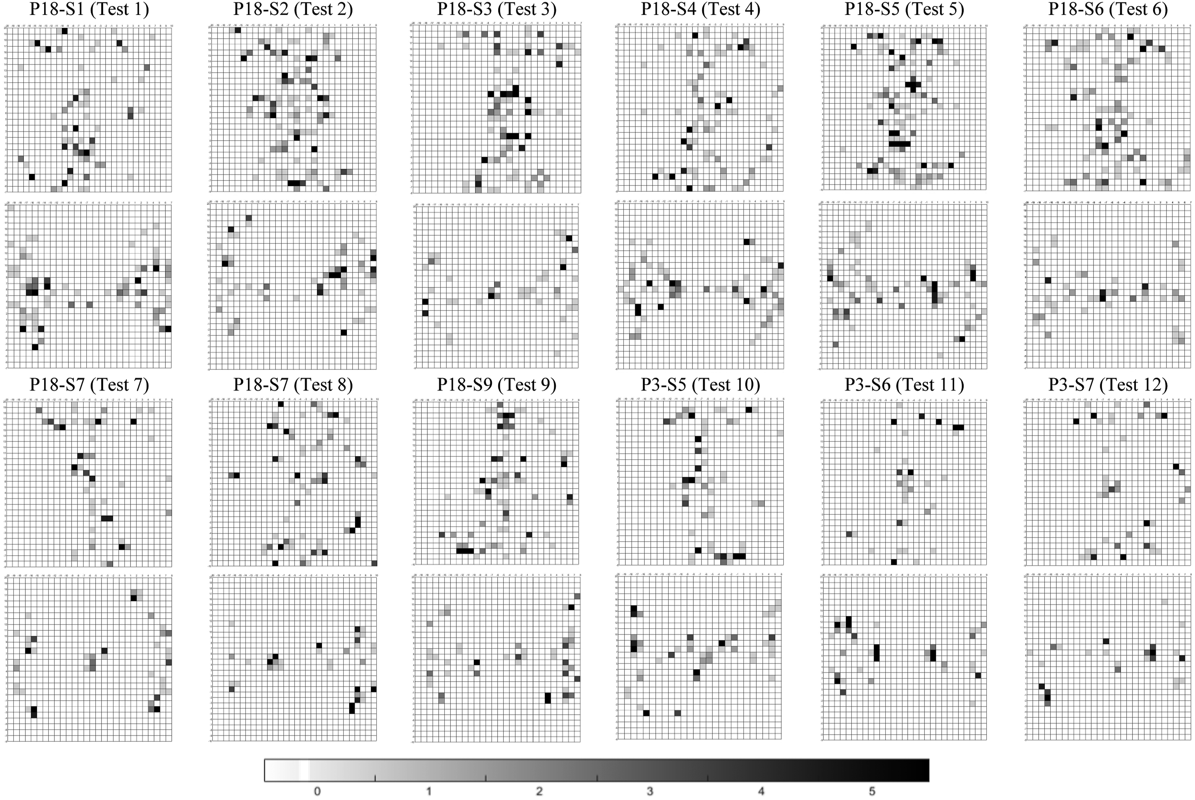
The quantitative crack information is processed by MATLAB-2 and binned scatterplots are output. These plots, included in Figure 9 (8-bit) and Figure 10 (16-bit), provide an at-a-glance indication of the overall condition of the specimens. However, the support span is not as obvious in the automated method plots as in the damage maps in Figure 8 (manual). This is because each square in the damage map represents ½ unit cell in the manual method (30 cells × 30 cells). In the automated methods, there is distortion due to the optimization of the block size reducing the number of blocks plotted for the 8-bit (20 cells × 20 cells) and for the 16-bit (26 cells × 26 cells), which means that portions of unit cells are merged together such that regions with longer or overlapping cracks may show with a higher intensity (darker color) in the damage map. The MATLAB-2 script was developed for the manual method, which outputs counts of cracks, while the automated methods output intensities related to the presence of cracks. Therefore, some refining of the MATLAB-2 damage map plotting script is necessary for the automated methods.

Figure 9.

8-bit automated method: damage maps for ½ max load (tests 1–6) and ⅓ max load (tests 7–12) full 3 × 3 in² (76 × 76 mm²) specimens are shown with spatially indicated quantities of horizontal transverse cracks (top) and vertical transverse cracks (bottom). The color bar indicates quantity of cracks.

Figure 10.

16-bit automated method: damage maps for ½ max load (tests 1–6) and ⅓ max load (tests 7–12) full 3 × 3 in² (76 × 76 mm²) specimens are shown with spatially indicated quantities of horizontal transverse cracks (top) and vertical transverse cracks (bottom). The color bar indicates quantity of cracks.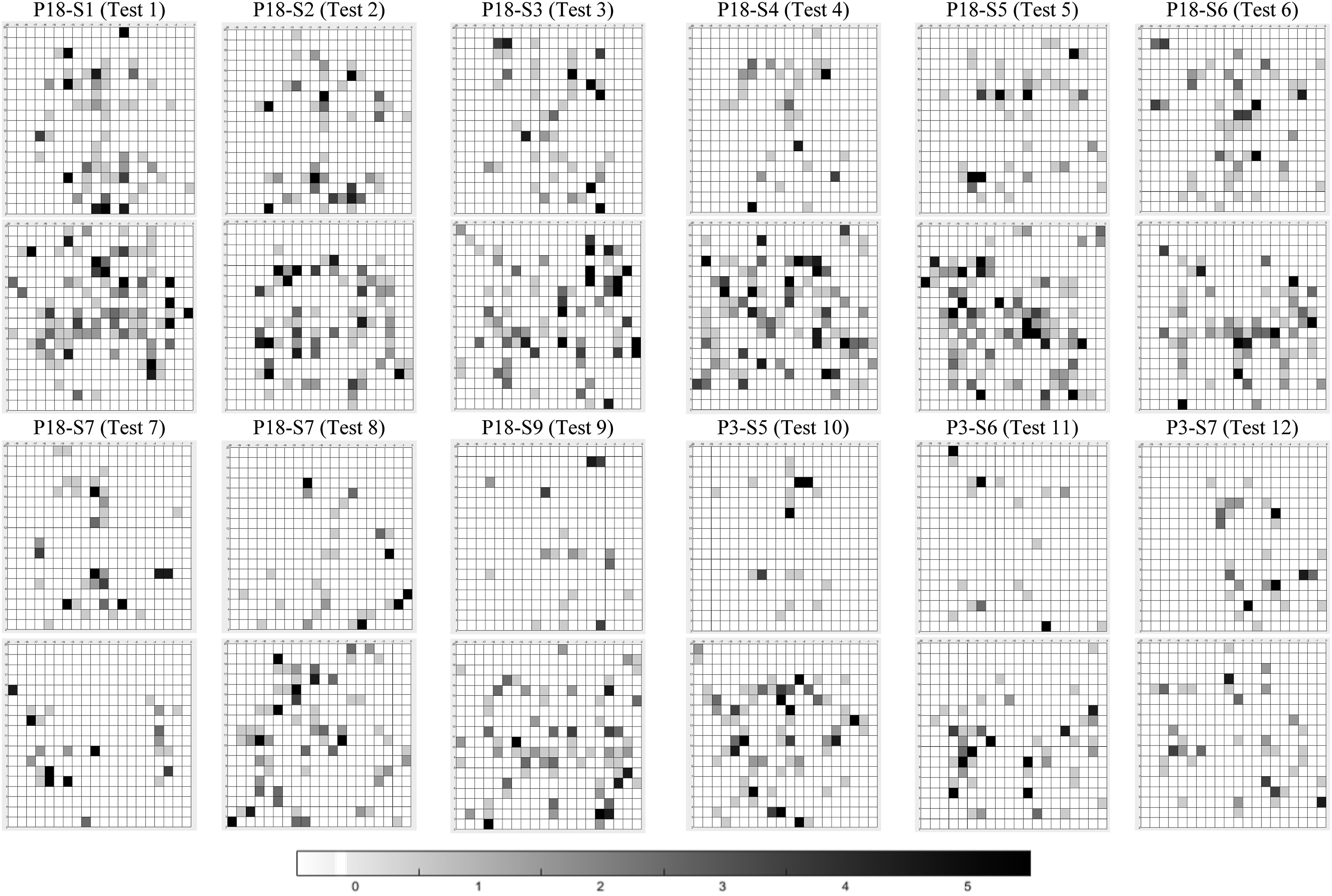

Conclusions

Two automated methods, an 8-bit and a 16-bit method, were presented for identifying and quantifying transverse cracks in a woven composite. These automated methods were evaluated by comparing with a control method in which transverse cracks were manually identified and counted. Quasi-static punch-shear experiments were conducted on 12 uniform specimens at two load levels, ½ of failure load and ⅓ of failure load, producing two damage states. Transverse cracks were qualitatively processed and quantitatively evaluated by each automated method and compared with the qualitative and quantitative results of the manual method.

Results of the 16-bit automated method appear qualitatively more similar to the experimental (unprocessed) and control (manually processed) results than do the 8-bit results, in terms of crack morphology, crack concentration within the support span diameter, crack shape and thickness, and the woven nature of cracks appearing in alternating unit cells. Both 8-bit and 16-bit automated methods are better able to find and count the number of cracks for conditions of greater damage. The 8-bit automated method was quantitatively more accurate than the 16-bit method. This indicates that a preprocessing step, present in the 8-bit method and not in the 16-bit method, aids in quantitative damage identification by reducing artifacts (sharp differences in contrast such as reflections, off-color yarns, dirt, and ink marks) that may lead to false positives or negatives.

Digital damage maps were produced for the manual method results, and these provide an at-a-glance view of the damage state of the specimen. Binned scatterplots were made for the 8-bit and 16-bit results, plotting intensity as an indicator of damage state (darker color means more damage). However, due to optimization steps, there is distortion resulting in portions of unit cells that are merged such that regions with longer or overlapping cracks may show with a higher intensity in the damage map. Additional work is needed to refine these plots into damage maps.

The manual method is fully hands-on, requiring an operator to count each crack, though this is the most accurate method (particularly if multiple users cross-check their counts). The 8-bit automated method has more processing steps, requires operator interface during the ImageJ preprocessing step, and is reasonably accurate when compared with the manual method. The 16-bit method eliminates the need for an ImageJ step and completes the analysis fully within MATLAB and so is more automated but less accurate. These automated methods are useful for a fast analysis of the damage state as indicated by the approximate magnitude of cracks generated by various means of quasi-static and dynamic damage generation including impact and other conditions. The automated methods described here for identifying transverse cracks can be performed from any adequately resolved image as an indication of this damage state. It is possible to extend this method into a portable platform, such as a mobile phone, for damage identification and quantification in the field. Field investigations at lower resolution could coarsely identify the damage state and indicate whether a higher fidelity study is needed. Future work should investigate the application of these methods to opaque and multilayer composites. Also of interest is how this approach could be applied to real-world structures, what specialized lighting and equipment may be required, and the development of standards and damage quantity references that could indicate structural health.

Supplemental Material

sj-pdf-1-jrp-10.1177_07316844211017647 – Supplemental Material for Automated detection and quantification of transverse cracks on woven composites

Supplemental Material, sj-pdf-1-jrp-10.1177_07316844211017647 for Automated detection and quantification of transverse cracks on woven composites by Christopher S Meyer, Enock Bonyi, Kyle Drake, Taofeek Obafemi-Babatunde, Aimanosi Daodu, Demilade Ajifa, Amber Bigio, Justin Taylor, Bazle Z (Gama) Haque, Daniel J O’Brien, John W Gillespie and Kadir Aslan in Journal of Reinforced Plastics and Composites

Footnotes

Declaration of conflicting interests

The author(s) declared no potential conflicts of interest with respect to the research, authorship, and/or publication of this article.

Funding

The author(s) disclosed receipt of the following financial support for the research, authorship, and/or publication of this article: This research was sponsored by the U.S. Army Research Laboratory and was accomplished under Cooperative Agreement Number W911NF-12-2–0022. The views and conclusions contained in this document are those of the authors and should not be interpreted as representing the official policies, either expressed or implied, of the U.S. Army Research Laboratory or the U.S. Government. The U.S. Government is authorized to reproduce and distribute reprints for Government purposes notwithstanding any copyright notation herein.

ORCID iD

Christopher S Meyer

Supplemental material

Supplemental material for this article is available online.

References

Talreja

. Damage development in composites: mechanisms and modelling. The Journal of Strain Anal Eng Des 1989; 24(4): 215–222.

Abrate

. Matrix cracking in laminated composites: a review. Composites Eng 1991; 1(6): 337–353.

Meyer

Haque

O’Brien

, et al. Mesoscale ballistic damage mechanisms of a single-layer woven glass/epoxy composite. Int J Impact Eng 2018; 113: 118–131.

Ogin

Brønsted

Zangenberg

. Composite materials: constituents, architecture, and generic damage. In: Talreja

Varna

(eds). Modeling Damage, Fatigue, and Failure of Composite Materials. Boston, MA: Woodhead Publishing, 2016, pp. 3–23.

Adams

Walton

Flitcroft

, et al. Vibration testing as a nondestructive test tool for composite materials. In: Wu

(ed). Composite Reliability, ASTM STP 5. Conshohocken, PA: American Society for Testing Materials, 1975, pp. 159–175.

Yan

Yam

. Online detection of crack damage in composite plates using embedded piezoelectric actuators/sensors and wavelet analysis. Compos Struct 2002; 58(1): 29–38.

Wang

, et al. FBG-based real-time evaluation of transverse cracking in cross-ply laminates. Compos Struct 2016; 138: 151–160.

Scholey

Wilcox

Wisnom

, et al. Quantitative experimental measurements of matrix cracking and delamination using acoustic emission. Compos A Appl Sci Manuf 2010; 41(5): 612–623.

Baker

Morscher

Pujar

, et al. Transverse cracking in carbon fiber reinforced polymer composites: modal acoustic emission and peak frequency analysis. Compos Sci Technol 2015; 116: 26–32.

10.

Pereira

Generazio

. Improved transverse crack detection in composites. Cleveland, OH: NASA. NASA Tech Memo 103261, 1990.

11.

Steiner

Eduljee

Huang

, et al. Ultrasonic NDE techniques for the evaluation of matrix cracking in composite laminates. Compos Sci Technol 1995; 53(2): 193–198.

12.

Kobayashi

Takeda

. Experimental and analytical characterization of transverse cracking behavior in carbon/bismaleimide cross-ply laminates under mechanical fatigue loading. Compos B Eng 2002; 33(6): 471–478.

13.

Garcea

Wang

Withers

. X-ray computed tomography of polymer composites. Compos Sci Technol 2018; 156: 305–319.

14.

Wilson

Chang

. Monitoring fatigue-induced transverse matrix cracks in laminated composites using built-in acousto-ultrasonic techniques. Struct Heal Monit 2016; 15(3): 335–350.

15.

Bradley

Soutis

, et al. A comparison of different approaches for imaging cracks in composites by X-ray microtomography. Philos Trans R Soc A Math Phys Eng Sci 2016; 374(2071): 1–15.

16.

Mohan

Poobal

. Crack detection using image processing: a critical review and analysis. Alexandria Eng J 2018; 57(2): 787–798.

17.

Bonyi

Meyer

Kioko

, et al. Assessment and quantification of ballistic impact damage of a single-layer woven fabric composite. Int J Damage Mech 2019; 28(2): 249–269.

18.

Gamstedt

Sjögren

. Micromechanisms in tension-compression fatigue of composite laminates containing transverse plies. Compos Sci Technol 1999; 59(2): 167–178.

19.

Gillespie

Hansen

. Transverse cracking of composite laminates with interleaves: a variational approach. Journal of Reinforced Plastics Composites 1997; 16(12): 1066–1092.

20.

Naik

Shrirao

Reddy

BCK

. Ballistic impact behaviour of woven fabric composites: Formulation. Int J Impact Eng 2006.

21.

Xiao

Gama

Gillespie

. Progressive damage and delamination in plain weave S-2 glass/SC-15 composites under quasi-static punch-shear loading. Compos Struct 2007; 78(2): 182–196.

22.

Gama

Gillespie

. Punch shear based penetration model of ballistic impact of thick-section composites. Compos Struct 2008; 86(4): 356–369.

23.

Bonyi

Kioko

Meyer

, et al. Toward automated identification and quantification of meso-scale damage modes in plain weave glass/epoxy composite laminates. Int J Damage Mech 2020; 29(5): 831–848.

24.

Rueden

Schindelin

Hiner

, et al. ImageJ2: imageJ for the next generation of scientific image data. BMC Bioinformatics 2017; 18(1): 1–26.

25.

Otsu

. A threshold selection method from gray-level histograms. IEEE Trans Syst Man Cybern 1979; 9(1): 62–66.

Supplementary Material

Please find the following supplemental material available below.

For Open Access articles published under a Creative Commons License, all supplemental material carries the same license as the article it is associated with.

For non-Open Access articles published, all supplemental material carries a non-exclusive license, and permission requests for re-use of supplemental material or any part of supplemental material shall be sent directly to the copyright owner as specified in the copyright notice associated with the article.

0.00 MB

0.73 MB