Assessment of cure cycle shortening for advanced composites via ultrasonics and dynamic mechanical analysis

Abstract

Composite materials are incorporated in various applications and their industry is widely growing. They offer cost savings and are more environmentally friendly than conventional metal structures. Some of the concerns this industry faces are the energy and time spent on long curing cycles to achieve permanent bonding between the matrix and fibers. In our previous work, a reusable sensing polytetrafluoroethylene (PTFE) system that can monitor the degree of cure of the composite while curing was developed and tested through Lamb waves analysis. This thin film is now used to monitor the same cure parameters for a shorter curing cycle than that suggested by the CFRP manufacturer. The results show that the three cure parameters: Minimum viscosity, full gelation, and vitrification are offset by the same time deducted from the cycle, highlighting the feasibility of using such technology. To verify the viability of this approach, tensile testing and dynamic mechanical analysis are performed on these composites. Tensile testing results show that the average tensile modulus for the shortened cycle is of similar values if not slightly higher than that of the normal cycle. Dynamic mechanical analysis (DMA) results verify both previous conclusions: Time shift of cure parameters and enhanced mechanical properties of the shortened cycle.

Keywords

Carbon fiber composites curing cycle cure monitoring non-destructive testing Lamb waves DMA

Introduction

The inclusion of fiber reinforced polymer composites (FRPs) in the automotive industry has grown significantly over the past decade as their usage moved from high-end niche vehicles to more affordable commercial cars and motorcycles. The presence of carbon FRPs in these vehicles is estimated to reduce the latter’s weight by 30–50%.¹ For example, the latest models in civil aviation, such as the Boeing Dreamliner and Airbus A350, are made of up to 52% CFRP.² This weight reduction has a remarkable impact on fuel efficiency and reductions in greenhouse gas emissions. In addition, CFRPs provide high specific strength and stiffness, corrosion and electrical resistance, low thermal expansion, good vibration damping characteristics, and superior fatigue and wear resistance than traditional metals.³ However, one major problem that the industry faces is that several manufacturers often provide curing cycles for the end customers based on trial and error. The cycles are not optimized to their fullest potential as they suffer from high safety factors that these companies establish.⁴ This struggle directly affects the consumers’ production time hence setting a drawback for the whole composites industry. Other problems facing the industry are mostly related to damages and air gaps appearing also during the curing process.⁵ This is why different methods exist for the monitoring of the curing process of the composites. In our previous work, a system that can effectively monitor the composites during curing using ultrasonic waves was implemented successfully.⁶ The goal here is to capitalize on that system to shorten the cure cycle time of the tested CFRP while making sure that the part is still cured properly.

Conventional resin cure monitoring methods include dynamic mechanical analysis (DMA), differential scanning calorimetry (DSC), rheology, and dielectric analysis (DEA).⁷ These techniques offer different curing parameters in their own prospect. Although they are all set up in a lab with ideal conditions, they are key for providing knowledge about glass transition temperature (T_g), cross-linking process progression, onset of cure, and degree of cure.⁸ They also give information about the glassy state transition (vitrification) and the progression of viscosity during curing.⁹ Stark tested various CFRP samples via DMA under different heating rates and damping frequencies to find how these parameters affect the state changes of the resin from liquid to rubbery, and then glassy state.¹⁰ Most in-situ cure monitoring research involves DEA as it is the most viable for this purpose. Hardis used DSC as a baseline comparison to determine the kinetic parameters of epoxy resin while establishing a relationship between T_g and the degree of cure from Raman spectroscopy and DEA under a single soaking temperature.¹¹ Kim and Lee developed a new method to monitor the cure of glass fiber/polyester composite by embodying a dielectric sensor and a thermocouple to measure the dissipating factor and temperature of the part.¹² Their method showed 70% matching compared to standard DSC. Two studies used a laboratory dielectric instrument to detect dielectric properties in conductive FRP composites samples during a resin transfer molding cure cycle.^13,14 Through a parallel plate, they measured these parameters through the thickness to evaluate the cure kinetics: minimum viscosity, gelation, vitrification, and full cure. Although all of these methods are widely used, they are usually limited to in-lab setups hence are not feasible at an industrial production and processing level.¹⁵ This is why research involving ultrasonic methods was popularized in the past two decades to study the resin curing cycle. One study monitored epoxy resin by exciting transducers to send and receive bulk ultrasonic waves and identifying the gelation and vitrification points respectively through amplitude and wave velocity curves.¹⁶ Wave velocity, being directly linked to the material stiffness, is an essential parameter in almost all research involving ultrasonics.¹⁷ On the other hand, viscosity of the curing resin was found to be related to the attenuation of the propagating wave.¹⁸ Lionetto and Maffezzoli determined the onsets of gelation and vitrification using air-coupled transducers as analyzed that the second onset happens when the kinetics of the reaction slow down while the latter becomes controlled by only diffusion.¹⁹ Hudson and Yuan made an interesting automated process to monitor the CFRP using guided Lamb waves.²⁰ Their analysis was based on only the amplitude graphs of mainly the antisymmetric A₀ mode of the propagating Lamb waves to determine all three cure parameters at several frequencies. Mizukami used a combination of signal processing for Lamb waves and a numerical micromechanics predictive model to respectively obtain attenuation and energy velocity then predict the CFRP complex modulus.^21,22 They also compared their predictions with DMA measurements to verify the validity of the proposed method. Liu used a Semi-Analytical Finite Element (SAFE) method and manufactured an FBG and PZT smart sensing film embedded within the laminate, to predict the modulus first then monitor it respectively. The film was later used to detect defects after curing.²³

To achieve serious cost savings and make advantage of the curing process of the composite laminate, it is essential to reduce the manufacturing time.²⁴ Hence, cutting the time suggested by the manufacturer of the curing cycle is crucial as it can also improve properties of the finished product, especially in unoptimized out-of-autoclave processes.²⁵ Numerically, Pantelelis developed a computational method to optimize and design the cure cycle of composites.²⁶ The method proved viability for several optimality criteria and the efficiency was demonstrated. Experimental cure cycle optimization techniques include the work by Dong on developing a rapidly cured out-of-autoclave resin then implementing it in a prepreg to minimize the curing cycle time with most optimized properties of the cured part.²⁷ Costa on the other hand, used DMA, DSC, and rheology to prove that slowing the heating rate of a certain composite from 5 and 10 to 2.5°C/min lowers the gelation temperature and slows down the rapid cure kinetics to better improve the cycle.²⁸ Other studies focused on optimizing the volume fraction of the fibers on one hand and getting rid of the voids and porosity on the other.^29,30 Hamdan focused on optimizing the manufacturing process as a whole and not just the curing time hence finding optimum pressure and temperature using numerical DOE (design of experiment) method.³¹

The focus of this article is to study the feasibility of the proposed technology when cutting down the curing time and analyze the properties of the composite when shortening the curing time. This investigation is done using a reusable flexible sensing film which encourages recycling and produces less material waste while keeping a faster pace in the setup, prior to the monitoring process. Matching acoustic impedance with resins, chemical inertness, and a high melting point are key factors that make Skived (PTFE) Polytetrafluoroethylene the best candidate for such sensing capabilities.³² This material, also known as Teflon, is usually used to integrate delaminations inside the composite laminates and study the wave changes after incorporating these artificial debondings.³³ Two thin PTFE layers sandwiching piezo-electric transducers (PZTs) would make a fine sensing network that adheres to the composite temporarily during curing while being reusable afterward.

This article first introduces experimental ultrasonic non-destructive evaluation of the cure cycle time change by explaining briefly the basics of Lamb waves and how the sensing network works to gather information needed for the monitoring of the cure successfully. Then, online monitoring of woven CFRP laminates is done by analyzing Lamb wave mode A₀ through velocity and amplitude curves before and after the cycle time shortening. Tensile testing is then done to prove that this time cutting does not affect the mechanical properties of the finished product. After that, dynamic mechanical analysis is used in its single cantilever setup to monitor the two cycles while curing, and to test for any T_g or static fatigue differences between them after curing. Eventually, the final verdict is concluded from the results of this traditional resounding method.

Ultrasonic non-destructive testing

Lamb waves fundamentals

In 1917, Horace Lamb published his deconstruction of elastic waves present in thin solid media that propagate by reflecting off the upper and lower boundaries of a plate thus expanding into two infinite sets of wave modes: symmetrical, and antisymmetrical modes.³⁴ Named after him, Lamb waves have complex properties that depend on the relationship between plate thickness and the wavelength.³⁵ The two sets of wave modes are made up of a superposition of longitudinal and shear vibrations, and their propagation characteristics vary with the excitation type, angle, and the structure shape itself.³⁶ 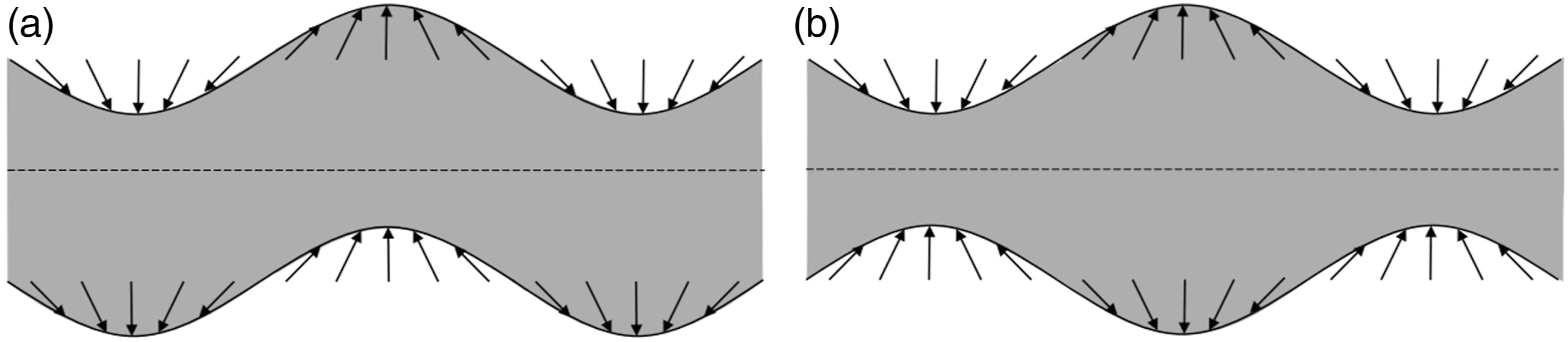Figure 1 shows the particle displacement of symmetric and anti-symmetric modes. Guided Lamb waves (guided along a certain path within the structure) have been used in many non-destructive testing (NDT) applications to assess the structural health of metallic and non-metallic structures. They are easily propagated once excited and have high sensitivity to damage. Their generation and data collection is relatively simple too. In many ways, Lamb waves have substituted conventional NDT tools because of their precise damage detection and localization.³⁸ Harb and Yuan assembled a fully non-contact system for identification of delamination in composite laminates and for imaging hardly visible damages in metallic plates, both using the basic antisymmetric A₀ Lamb wave mode.^39,40 Tarraf and Fakih scrutinized the effect of plastic deformation within metal plates joint by friction stir welding on the propagation behavior of guided Lamb waves to assess the material discontinuity in this weld application.^41,42

Figure 1.

Displacement of particles in an (a) antisymmetric and (b) symmetric Lamb wave modes. The median dotted line of the plate is shown.³⁷

Lamb waves are dispersive, which means that the velocity of each mode is not constant, but dependant on the excitation frequency.⁴³ In our work, frequencies usually vary between 50 and 300 kHz, which, for a thin CFRP plate (aprox. 1 mm thickness), makes the set of Lamb waves consist of only the first symmetric and asymmetric modes: S₀ and A₀, making the signal processing less complex. Usually, S₀ is faster than A₀ at low ultrasonic frequencies. As the frequency increases, S₀ velocity decreases while that of A₀ increases, as they both converge towards each other in values transforming into a Rayleigh-Lamb wave.⁴⁴ Also, these modes propagate with different displacement amplitudes, making each frequency denoting an amplitude dominant mode over the other regardless of their speeds. All these variants make Lamb waves complex to work with but also easy to distinguish once understood and analyzed. In this work, the frequency used to excite the CFRP laminate is 70 kHz for which the A₀ is at its highest respective strain compared to S₀. The choice to work with A₀ derives from the fact that it propagates in an out-of-plane fashion, making it more suitable to propagate through the sensing film and into the CFRP laminate. Whereas, the S₀ mode, propagating in-plane, loses much of its amplitude when transmitting from one material layer to another.

Ultrasonic measurements

Figure 2 shows the CFRP prepreg layup within the oven with all the bagging components. Two 0.25 mm thick Skived PTFE layers sandwich two PZTs: one actuator and one sensor. This sensing sandwich is placed directly in contact with the laminate as it adheres to it temporarily during curing while under vacuum giving very good signal propagation inside the CFRP and then is removed easily after the curing cycle is done and the bagging is opened. The PZTs used are disc shaped PZT-5J material type with 0.5 mm thickness, 7 mm diameter, and have a Curie temperature of 320°C, which means that they are effective up to 160°C. The CFRP laminate consists of three layers of out-of-autoclave XPREG XC110 woven prepreg. It is 220 mm³ × 350 mm³ × 1 mm³ in dimension. The sensing film is of the same length and width, and the PZTs inside are distant 240 mm from each other along the 0° direction of the fibers.

Figure 2.

Composite layup process with the bonded sensing film layer.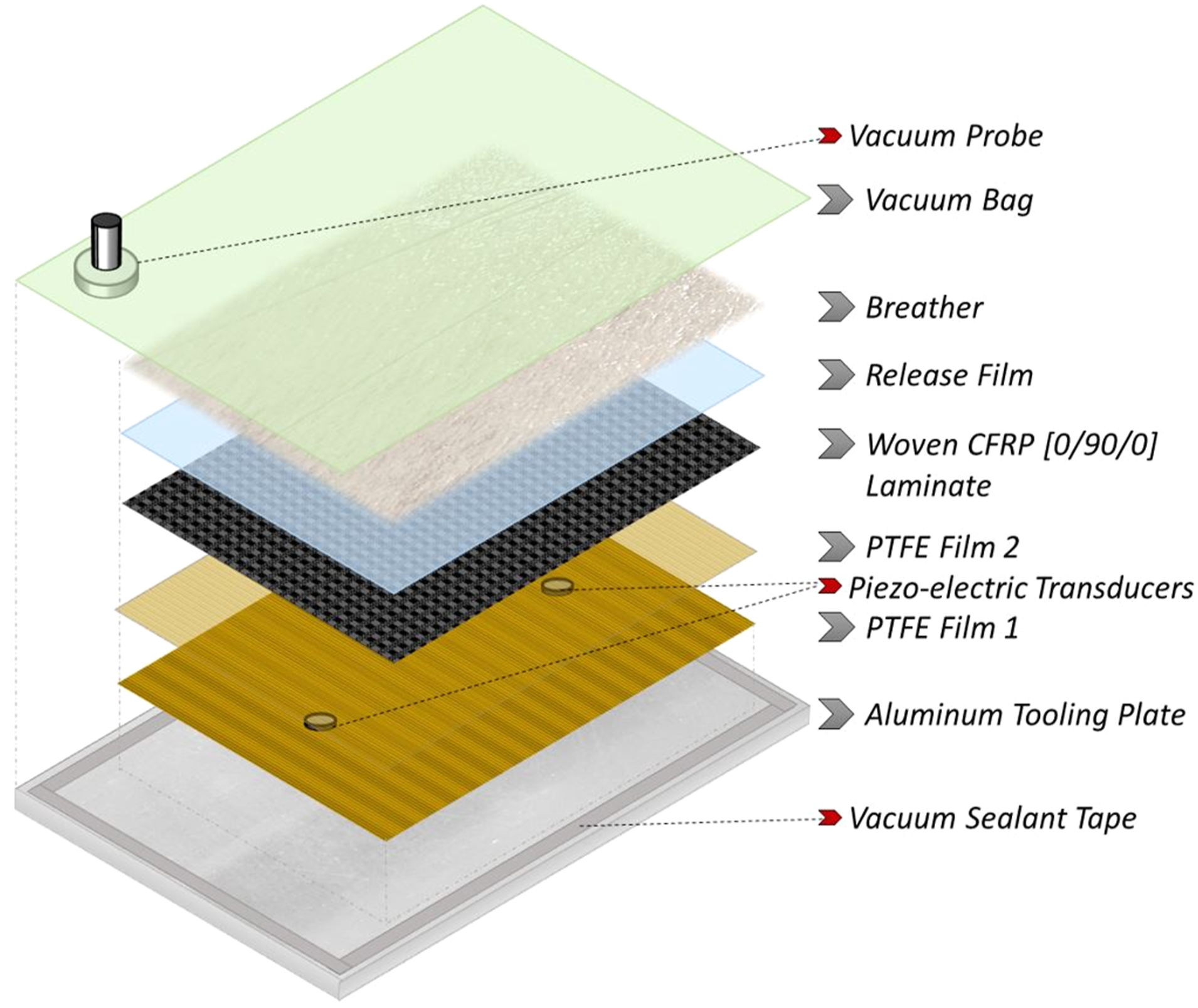

The layed up composite goes into the oven according to the curing cycle set by the manufacturer and shown in Figure 3 (4hr-soak). The temperature ramps up from room temperature to 70°C in 50 min then soaks at this temperature for 4 h before ramping up again to 120°C within 25 min, soaking for 1 h and then cooling naturally. The cool down shown in the figure is in just 1 h, whereas there is no cooling system inside the oven. The part cools naturally therefore it takes up to 3 h for the laminate to fully cool down (exponential decay).

Figure 3.

Cure cycle proposed by the manufacturer (4hr-soak) and the shortened cycle tested (3hr-soak) shown with vacuum pressure in an out-of-autoclave setup.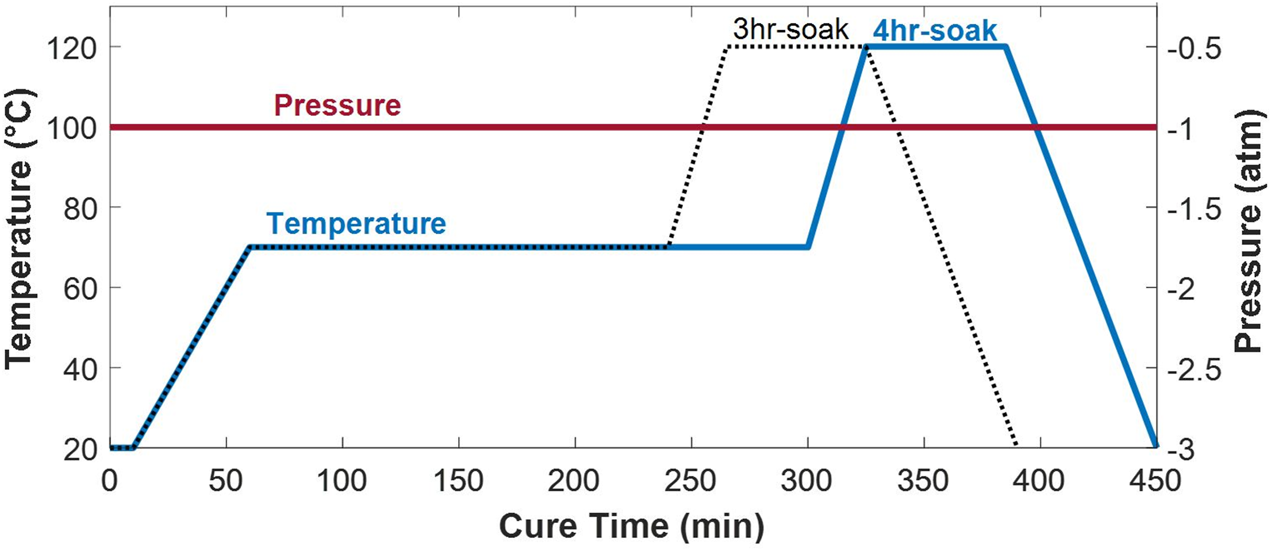

To excite Lamb waves during curing, the actuator PZT is soldered to a wire attached to the amplifier which intensifies the five-peak sinusoidal Hanning-windowed signal generated by a signal generator. The wave then travels within the CFRP laminate reaching the sensor PZT which is wired to an oscilloscope, recording any measured signal. The amplified signal to the actuator is 160 Vpp (peak-to-peak voltage) at a central frequency of 70 kHz. This frequency was chosen after some testing as it provides highest A₀ amplitude and barely records S₀. Data were being recorded by the oscilloscope every 10 min.

The cure cycle shortening is cut from the longest soak of the cycle, the first one. The modification is cutting one full hour of the 4 h soak period at 70°C, making it a 3hr-soak period. This was done based on a conclusion from previous work where the cure parameters were present in the second ramp and second soak stages following the end of this first (4 h) soak period.⁶ Hence the total time of the modified curing cycle would now be 390 min instead of 450 min. The 3hr-soak curing cycle is also shown in Figure 3 in the dotted line. The data for both cycles are analyzed through two parameters: A₀ mode group velocity and its amplitude. From previous conclusions, the three curing parameters (minimum viscoscity, gelation, and vitrification) are all present in both curves, but the first two appear better in the amplitude curve while vitrification is distinguished more clearly in the velocity curve.

The group velocity is basically the distance between the transmitting and receiving transducers, covered by the propagating signal, divided by the time of flight between the actuated packet of signal and the first received A₀ mode packet. Figure 4(a) shows the time of flight covered by the first received A₀ packet. The third peak of the wave packet is chosen to calculate the time of flight since it is the highest peak in the five-peak sinusoidal Hanning-windowed signal generated. Although the actuated signal is not shown in the figure, the electromagnetic noise is usually overlapping with it time-wise therefore it is a good estimation to look at it instead; however the calculations are based on the actual generated signal. Figure 4 shows the direct comparison of signals at the three cure parameters points and one final data point at a typical glassy state (minute 390 or 450 for the 3hr-soak and 4hr-soak experiments respectively).

Figure 4.

Raw data points from the curing experiment comparing cure stages for both cycles.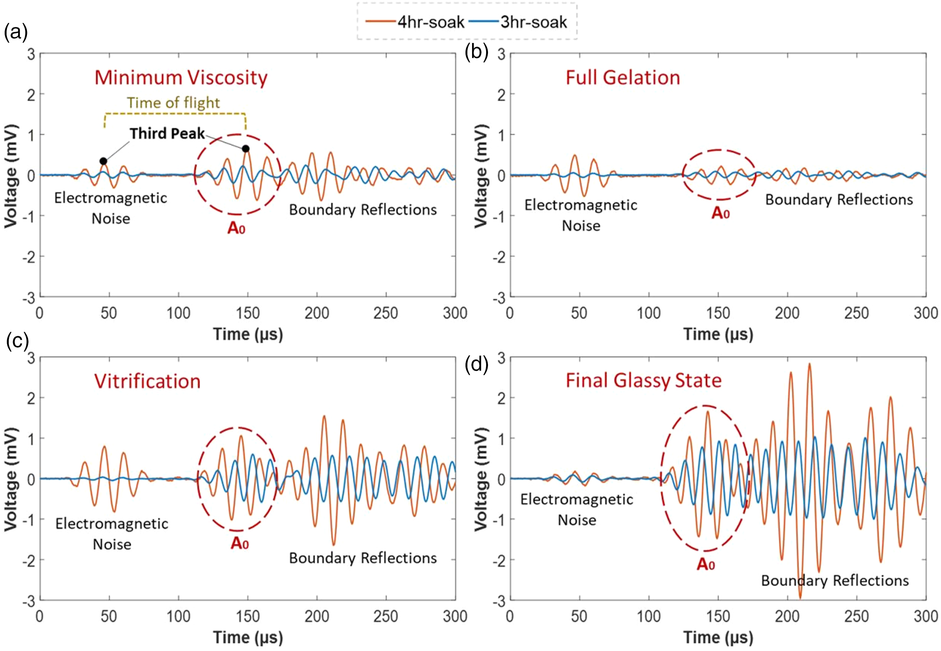

Figure 5 shows the group velocity and voltage curves for both 4hr-soak and 3hr-soak experiments. They follow the same trend, and the 1 h shift between them is noticeable after the end of the first soak at 70°C. The cure parameters are deduced for both cycles as follows: The minimum viscosity point is the maximum the end of the first soak. That is where the viscosity of the whole composite, not the resin, is at its lowest; full gelation occurs at the minimum after that, where the viscosity is at its highest in this rubbery region; then vitrification occurs on the change of slope during the ascent. The latter point is more reliably taken from the velocity curves while the minimum and maximum viscosity (gelation) points are better determined from the voltage curves. Clearly, all three points are shifted exactly by 60 min backward in the 3hr-soak experiment: vitrification moving from 365 to 305 min, full gelation from 335 to 275 min, and minimum viscosity (always at the end of the long soak-therefore redundant) from 300 to 240 min. This means that the reduction of the first soak period by 1 h kept the curing process functioning normally for the rest of the cycle.

Figure 5.

Group velocity and voltage of A₀ mode generated and received over the [0/90/0] woven laminate for the 4hr-soak and 3hr-soak experiments.⁶

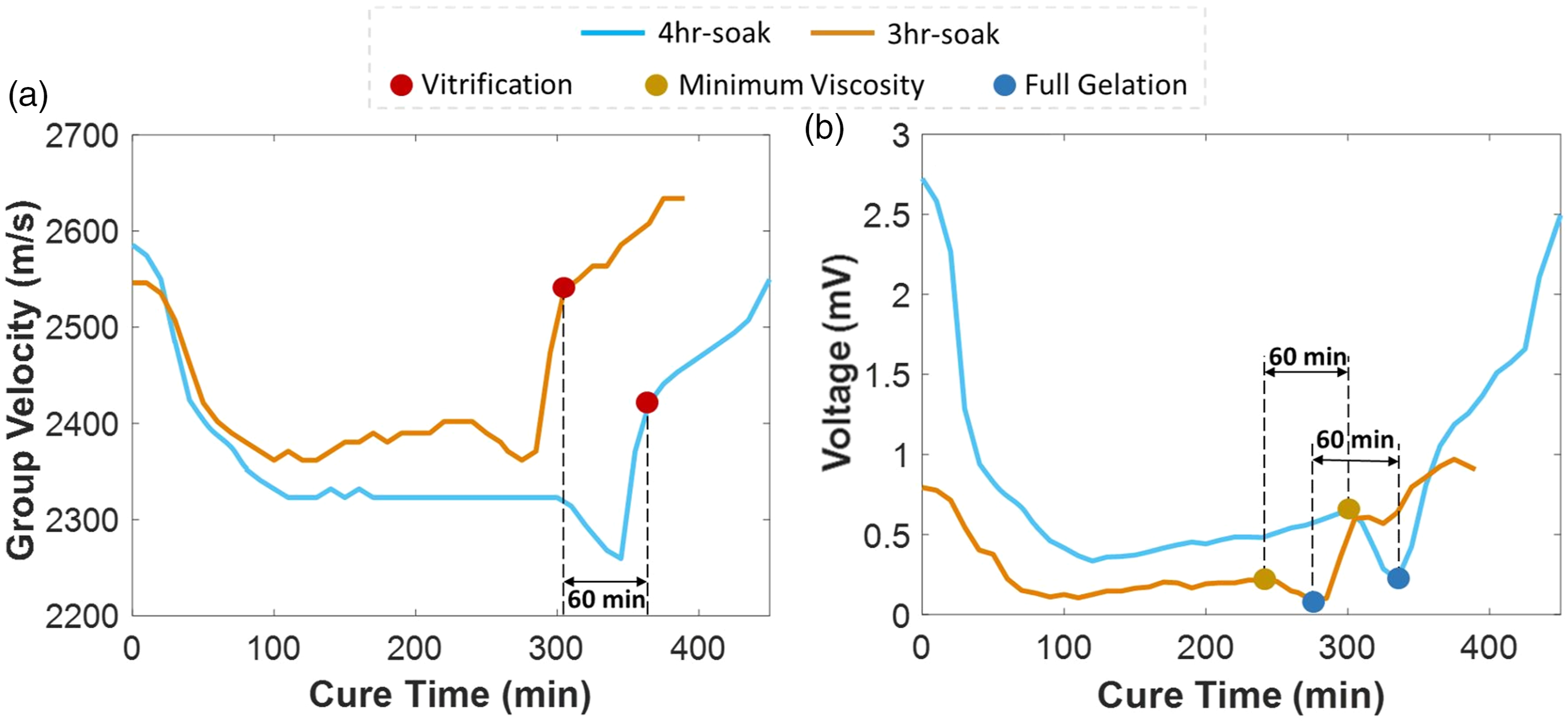
The trends seen in Figure 5 are very similar but the range of values differs from one experiment to another. For example, the velocity curve in the new 3hr-soak cycle starts at a marginally lower value than that in the 4hr-soak experiment but after 20 min it surpasses the latter for the rest of the cycle. On the other hand, the amplitude curve of this A₀ wave mode in the 3hr-soak experiment is always lower than that in the 4hr-soak experiment. Several reasons may cause these slight differences in values: Minor difference in the layup, inconsistency in the bonding between the sensing film and the layup, or the effect of the shelf life on the CFRP prepreg since the two cycle experiments were tested separated by a long period of time. These inconsequential variations in the curves amplitude have little meaning, however. The importance of this cure monitoring method is in the trend of the curve and the time of the cure parameters derived from these curves. After verifying that the cycle reduction of the CFRP kept the curing normal according to the cure parameters deducted by the ultrasonic cure monitoring, more proof is required to make sure that the mechanical properties are kept intact after the part is cured.

Tensile testing

The simplest way of inspecting some mechanical properties of the used CFRP is by doing a tensile test which mainly gives information about the tensile strength and the tensile modulus (Young’s) of the material. Samples were prepared according to ASTM standards which suggest 25 cm long and 2.5 cm wide samples for the woven composite while leaving some freedom in choosing the thickness (according to the number of laminas) and the tab length (according to the tab material used).⁴⁵ Since the layup in the cure monitoring experiments always consisted of three layers with [0/90/0] orientation, the same is ought to be used in the samples which makes the thickness around 1 mm. The orientation of the laminas in the tensile testing samples is [0]₃ since this will directly give the Young’s modulus in the first direction of the fibers although the woven nature of this CFRP makes the 0° and 90° directions in-plane have almost the same properties hence it is directly comparable to the previous ultrasonic-experiment layup.

On this basis, ten specimens were made for each curing cycle, laid-up and cured with 1.5 mm thick aluminum tabs on each end of the specimen on both sides (four tabs for each specimen). The tab is 6 cm long and 2 cm wide. Adhesive layers were placed between the tabs and the specimens to ensure bonding while curing. These tabs are essentially used for eliminating slippage of the samples from the UTM grips while the test is running. After curing, the specimens are trimmed properly and each one is tested in the UTM at a 1 mm/min rate. The distance between the two strips of reflective tape, known as gage length, is set to be 10 cm. These white strips are placed to measure the strain in the sample using the laser vibrometer.

Figure 6 shows the first set of five samples for each cure cycle after curing and trimming. Tensile tests are then carried out for all the samples until failure which happens “suddenly” (fracture) since this is a brittle material. The results of the test show the stress–strain curves which have a direct relationship with the modulus (the slope). The latter is calculated via the insertion of a linear trendline since the curves are almost linear in this brittle test. For the same last reason, the ultimate stress (highest stress on the curve) is the same as the tensile strength since there is no yielding in this case. Figure 7 shows four distinct stress–strain curves, two for the 4hr-soak cycle and two for the 3hr-soak cycle of random specimens.

Figure 6.

Some samples after cure and trim, before tensile testing.

Figure 7.

Stress–strain curves for four random tensile-tested specimens.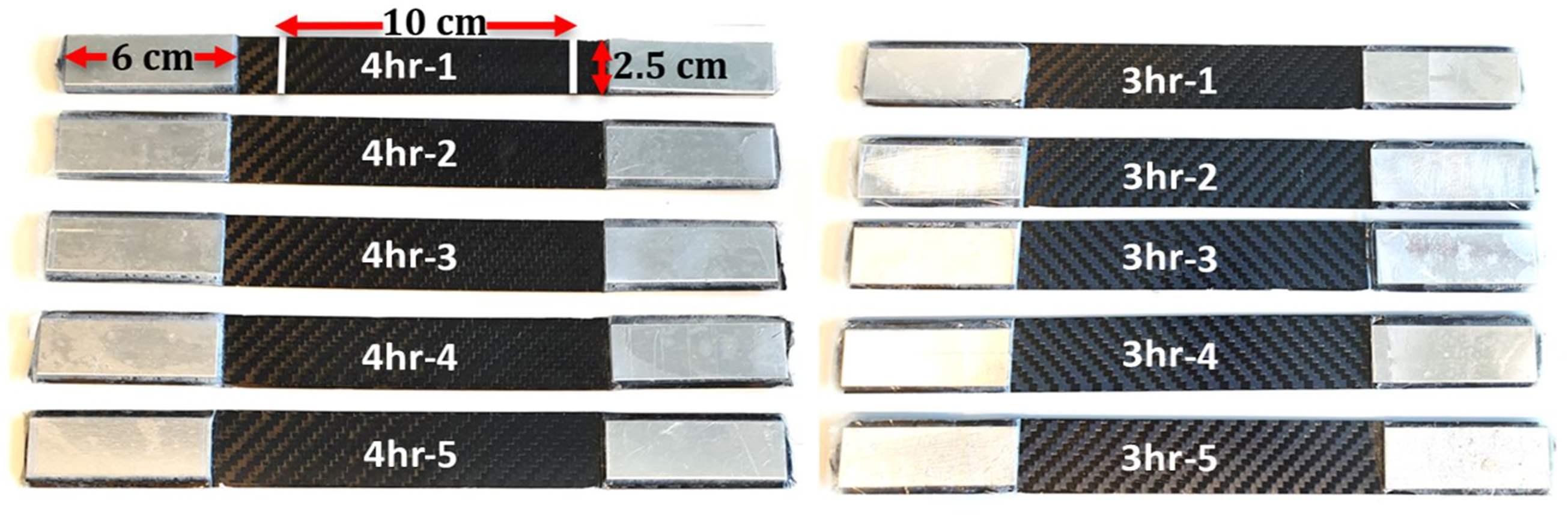

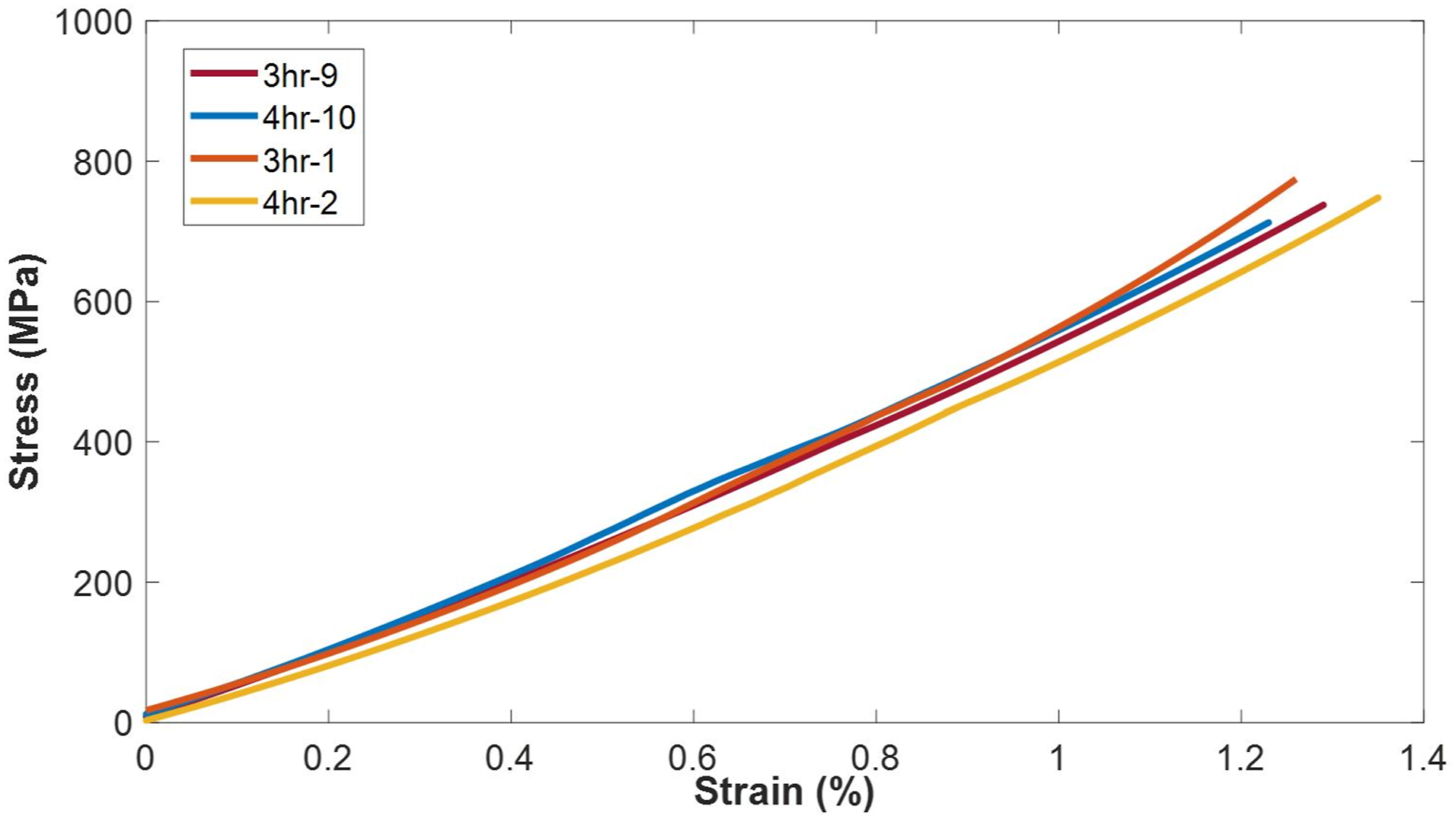
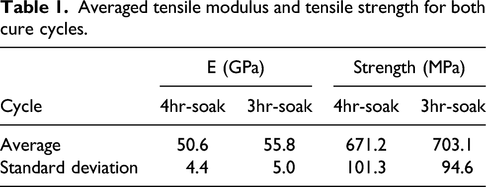
Figure 8 summarizes the tensile test results. It shows the Young’s modulus (8.a) and the strength (8.b) of the material for each specimen for both curing cycles. The averaged tensile modulus and tensile strength for both cure cycles specimens are shown along with the standard deviation in Table 1. The averaged E for the regular 4hr-soak cycle is 50.6 GPa while that of the modified 3hr-soak cycle is higher at 55.8 GPa. The same can be said for the averaged strength as they compare at 671 and 703 MPa, respectively. While the standard deviation is very close in both cases, it can be said that the cycle modification is in fact an enhancement not only by cutting time but also by improving mechanical properties to an extent, especially the tensile modulus. These values should be compared to that of the manufacturer where they claim the tensile modulus to be 55.1 GPa (very close to the 3hr-soak cycle average) and the tensile strength to be 645 MPa (exceeded in both cycles). The enhanced mechanical properties in the trimmed cycle could be due to better and more optimized cross-linking between the matrix and the fibers during curing, especially since the cycle proposed by the manufacturer usually has a safety factor large enough to actually lower the efficiency of this cross-linking.⁴⁶

Figure 8.

Results of the tensile test for all specimens for both cure cycles.

Table 1.

Averaged tensile modulus and tensile strength for both cure cycles.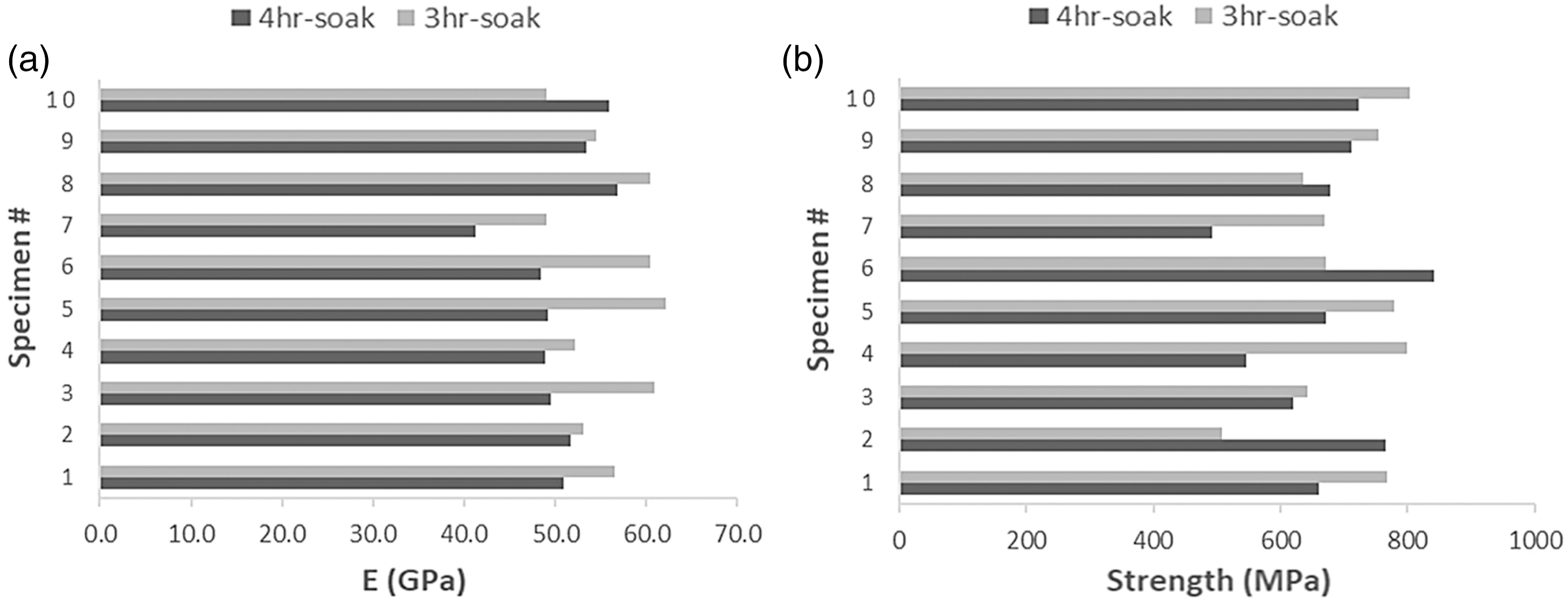

	E (GPa)		Strength (MPa)
Cycle	4hr-soak	3hr-soak	4hr-soak	3hr-soak
Average	50.6	55.8	671.2	703.1
Standard deviation	4.4	5.0	101.3	94.6

Dynamic mechanical analysis

To further prove the effectiveness of this cycle time shortening, a DMA machine was used to test both cycles for small woven CFRP specimens. DMA measures the complex modulus and compliance as a function of temperature, time, and frequency. Thermoset properties measured include storage and loss modulus, storage and loss compliance, tan δ and several more. Tan δ is the phase lag between stress and strain (the ratio of loss modulus over storage modulus), and a typical measure of damping or energy dissipation.⁴⁷

The most common use for DMA is to get the glass transition temperature T_g. It can also be used to monitor the curing cycle of any polymer. For the latter use, the same cycle can be implemented inside the machine with the addition of a sinusoidal constant strain at a single or several frequencies.⁴⁷ In order to compare this reliable method with the ultrasonic method used in this work, the same cycle is used on the woven prepreg to differentiate the cure parameters. Figure 9 shows the setup of the DMA experiment inside the PerkinElmer DMA 8000. A couple of differences between the oven-cured CFRP and the DMA-tested CFRP are present. First, the size of the sample in DMA (30 mm³ × 10 mm³ × 1 mm³ using the same [0/90/0] layup) is much smaller than the original cured plate size and has a much larger thickness to length ratio than the latter. Second, during the DMA test, a constant straining vibration of the specimen is used at a frequency of 1 Hz in a single cantilever setup with initial force and displacement of 2 N and 0.05 mm, respectively. This cyclic loading is required for the calculation of the gain and loss moduli during the cycle. Last, the specimen in the DMA furnace chamber cannot be set under vacuum which is essential to the proper cure and the acquisition of good mechanical properties in the CFRP. However, this test is only performed to verify the previous cycle trimming and its inertness regarding the cure parameters. Therefore, two sets of specimens were tested, some for the regular 4hr-soak cycle and others for the new 3hr-soak cycle.

Figure 9.

Setup of DMA experiments showing the specimen in single cantilever mode.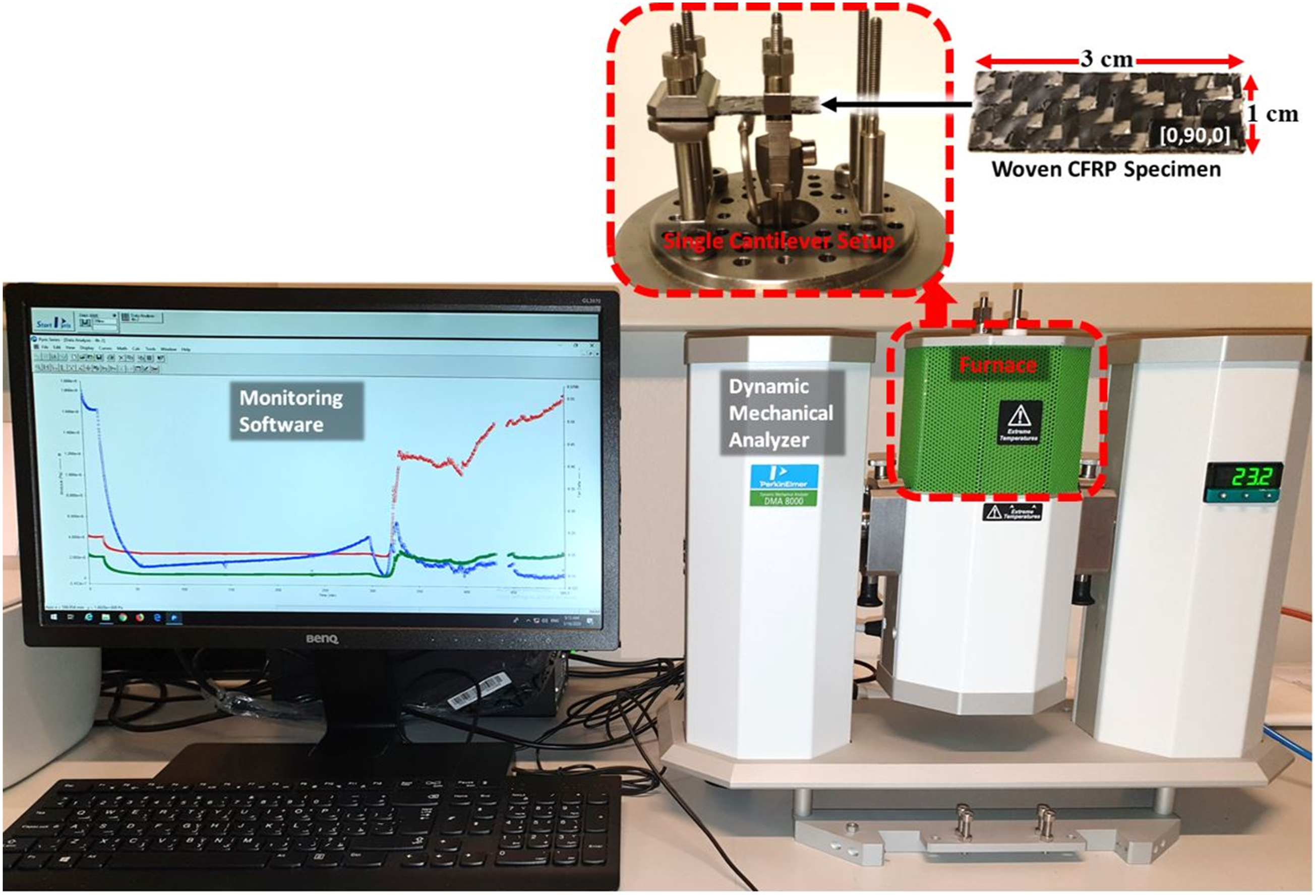

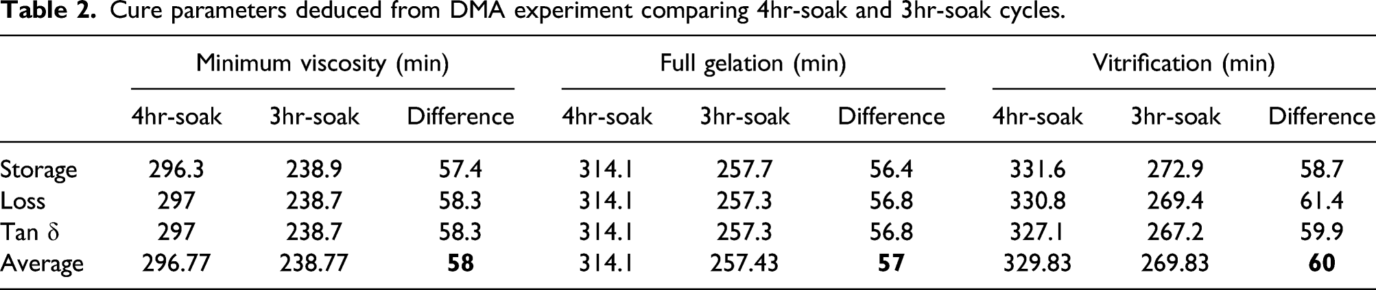
The graphs in Figure 10 show the storage and loss moduli, E^′ and E^″ respectively, and tan δ (E^″/E^′) with respect to curing time for both cycles. The trends of these curves at first glance replicate directly the trends of the previous ultrasonic curves with the three main cure parameters clearly present as denoted in black dots. Table 2 summarizes the time values of these points concerning both cycles and all three represented curves. Each given time in the table is averaged for five different specimens for each curing cycle. The average time difference between the vitrification onsets of both cycles is 60 min while full gelation and minimum viscosity are shifted by 57 and 58 min, respectively. This is more reliable and accurate since data is taken every second, whereas in the ultrasound case, it was taken every 10 min; hence, the minor difference in 2–3 min. This 1 h shift between the cure parameters of the two cycles further proves the effectiveness of this cycle shortening. However, comparing these times to the ultrasonic ones, the minimum viscosity of the resin occurring at the end of the first soak is still present at the same time while gelation is shifted earlier by approximately 20 min and vitrification also occurring earlier by almost 35 min for both cycles. This could be due to several reasons, some of them are mentioned in the previous paragraph: Having different length-to-thickness ratios than the original plates, no vacuum, and cyclic loading at a constant frequency. Also, the small specimen in the furnace is molded by the temperature faster and better than the respectively larger CFRP plate that is in a large oven surrounded by the vacuum bag, Teflon, and a thick aluminum plate. This time shift in the last two cure parameters between the oven-cured, ultrasonically tested plate and the DMA-tested specimen can also be considered as a safety factor for the cure cycle, meaning it would be safe to say that the part is cured if the ultrasound cure parameters are present within the cycle.

Figure 10.

DMA results showing loss factor, gain and loss moduli versus cure time for both cycles.

Table 2.

Cure parameters deduced from DMA experiment comparing 4hr-soak and 3hr-soak cycles.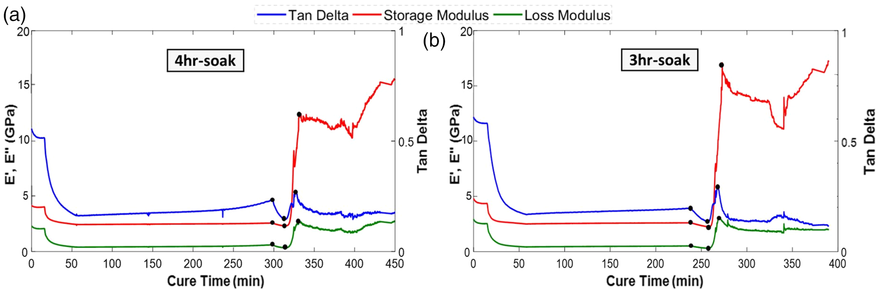

	Minimum viscosity (min)			Full gelation (min)			Vitrification (min)
	4hr-soak	3hr-soak	Difference	4hr-soak	3hr-soak	Difference	4hr-soak	3hr-soak	Difference
Storage	296.3	238.9	57.4	314.1	257.7	56.4	331.6	272.9	58.7
Loss	297	238.7	58.3	314.1	257.3	56.8	330.8	269.4	61.4
Tan δ	297	238.7	58.3	314.1	257.3	56.8	327.1	267.2	59.9
Average	296.77	238.77	58	314.1	257.43	57	329.83	269.83	60

As for the variance in values between the curves of each cycle, all three curves start at a slightly higher value for the 3hr-soak specimen, this is due only to the specimen itself. The loss modulus and tan δ resemble their counterparts in the two cycles for the rest of the curing time. However, the storage modulus, which indicates mainly the complex dynamic modulus of the specimen (since the loss modulus is very low), ascends to a higher value during the transition from rubbery to glassy state (before vitrification onset) in the 3hr-soak cycle than in the regular 4hr-soak cycle. Then, it keeps on rising at a slower rate after entering the glassy state for both cycles while the 3hr-soak reaching a higher value of around 17.5 GPa compared to 15 GPa in the 4hr-soak cycle case. This affirms the previous results concluded from the tensile test that the mechanical properties of the CFRP at the end of the new shortened cycle are improved. These values for the moduli are low when compared to 51 and 56 GPa for the 4hr-soak and 3hr-soak cycles, respectively, from the previous tensile test. In fact, Stark tested another carbon fiber prepreg during curing in a DMA machine between −90 and 280°C.⁴⁸ At the minimum temperature, the storage modulus was high at 45 GPa but within the temperature range used in this experiment (above room temperature), the storage modulus had a similar maximum to this experiment (around 15 GPa). This mechanical property value decrease in the DMA, while the CFRP is curing inside could be due to the absence of vacuum within the furnace and the extensive dynamic strain on the specimen while it is curing. This, however, does not affect any of the conclusions as it is sufficient in this test to check for the trend of the curves and compare the cycles to each other.

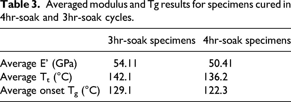
Curing CFRP inside the dynamic mechanical analyzer is not the most traditional use in DMA testing. Conventionally, DMA is used in a heating ramp cycle while oscillating at a constant or varying frequency to find T_g, the glass transition temperature, of these polymer composites. Thus, two sets of specimens of the same size mentioned above were cured in the oven separately, each by one of the two cycles. After proper curing, these specimens were tested in the DMA machine on a 10°C/min temperature ramp from 25 to 180°C and at a frequency of 1 Hz with initial force and displacement of 2 N and 0.05 mm, respectively, to get both the initial storage moduli and the glass transition temperature. Traditionally, T_g is found in two ways, either from the tan δ peak, or from the first onset of the storage modulus curve drop. The manufacturer states that T_g calculated from the storage modulus curve onset is 121°C, whereas the T_g found from the tan δ maximum (usually denoted T_t) is 135°C. The results are summarized in Table 3 below. This table shows the averaged values of at least five specimens tested for each cycle. The storage moduli found are comparable to the previous tensile testing results with 54.1 and 50.4 GPa, respectively, for the 3hr-soak and 4hr-soak cycles, whereas the Young’s moduli found previously were 55.8 and 50.6 GPa, respectively. This confirms that the mechanical properties conclusions from the previous experiment are intact at this smaller scale in the DMA machine. As for T_g, in the original 4hr-soak cycle results, the values of 122 and 136°C are very close to the manufacturer’s (difference by only 1°C). In the 3hr-soak case, onset T_g and T_t are 129 and 142°C, respectively, which are also higher than those of the 4hr-soak cycle. This, and the modulus change, could be due to better cross-linking in the curing of the shortened cycle, and/or a more stress-relaxed composite rubber after the additional 1 h in the original cycle, resulting in better mechanical and thermal properties for the shortened cycle. Figure 11 shows the averaged storage modulus and tan δ curves for the woven CFRP specimens of both cycles. Notice that the storage moduli in Table 3 were found using many more samples that were tested isothermally only and are not shown in Figure 11. This is why in the averaged curves the storage moduli values at the start of the temperature ramp are different from the storage moduli values in the table.

Figure 11.

DMA temperature ramp results for oven-cured specimens showing averaged storage modulus and tan δ curves for both cycles.

Table 3.

Averaged modulus and Tg results for specimens cured in 4hr-soak and 3hr-soak cycles.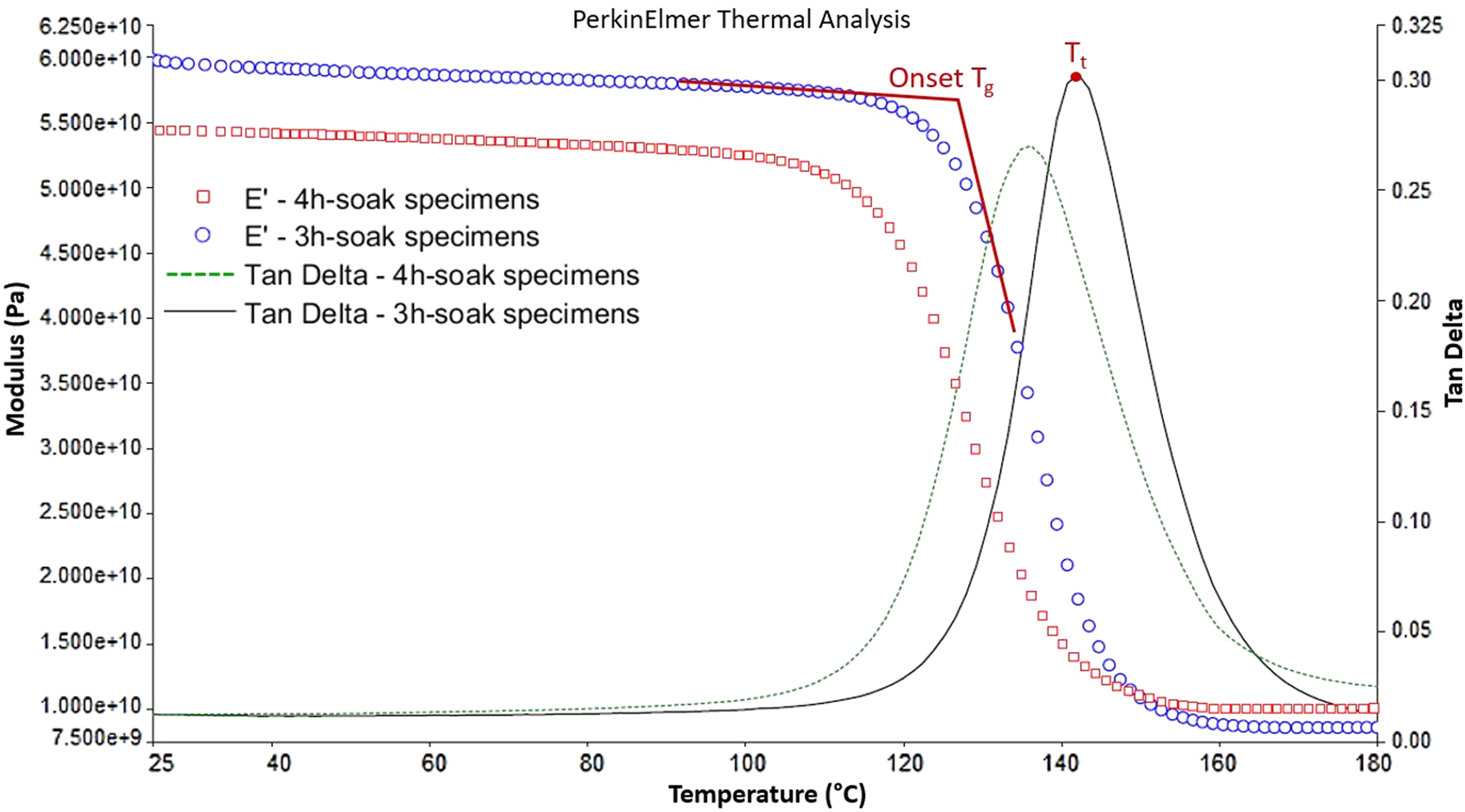

	3hr-soak specimens	4hr-soak specimens
Average E’ (GPa)	54.11	50.41
Average T_t (°C)	142.1	136.2
Average onset T_g (°C)	129.1	122.3

One final use of the DMA machine is to test for creep and compare both cycles in terms of static fatigue properties. Creep is the tendency of a material to strain gradually or deform permanently when constant stress, lower than the strength of the material, is applied.⁴⁹ Therefore, it is a time-dependent form of deformation. After long periods of time, and depending on the properties of the material, creep can lead to static fatigue failure, known as rupture.⁵⁰ To compare creep testing for the two cycles in a relatively short period of time, heat should also be added since high temperature expedites the severity of the creep process. Thus, the following experiment was conducted in the DMA machine. Two sets of three specimens, each cured in one of the two cycles, were tested at three different temperatures each: Room temperature, T_t temperature, and one in between. The manufacturer T_t temperature is 135°C. At this temperature, the CFRP is clearly rubbery since it surpassed the onset T_g temperature of 121°C and exceeded its service temperature given by the manufacturer (115°C).

The tests are conducted in a way that each specimen will strain for 5 min under minimal loading (0.1 N) before promptly increasing the load to 6 N and maintaining it for 20 min, then going back to the minimal loading for another 5 min. After that, the temperature will increase from 25 to 80°C and the specimen will be loaded in the same previous fashion for 30 min. Then, the process is again repeated at 135°C. This type of loading is not bound by frequency since it is held statically. Figure 12(a) shows each specimen’s strain versus time during the creep test, and Figure 12(b) shows the averaged strain curves for the 3hr-soak and 4hr-soak cycles specimens. In the latter, it is clear that the response at room temperature is very similar in both averaged curves. After applying the high load at 80°C, the 3hr-soak curve strains less than the 4hr-soak one by an average of 0.03% strain, before also bouncing back to a lower value in the post-load region of 0.1 N. At 135°C, the pre-loaded and post-loaded regions are very similar in both cycles, almost returning to 0.005% (negligible) strain at the end of the experiment. However, within the high-loaded region at this temperature, the 3hr-soak average curve response is much lower than that of the 4hr-soak curve (an average of 0.1% strain difference). This shows that although almost all specimens bounce back to a regular state after loading, the response of the 3hr-soak cycle specimens to this creep test is similar if not better than that of the 4hr-soak cycle specimens; thus, confirming that this cycle shortening did not diminish the static fatigue performance of the tested composite. Rather, it might also have improved it.

Figure 12.

Creep test results for (a) all specimens from both cycles, and (b) averaged curves for each cycle, also showing temperature and loading schemes.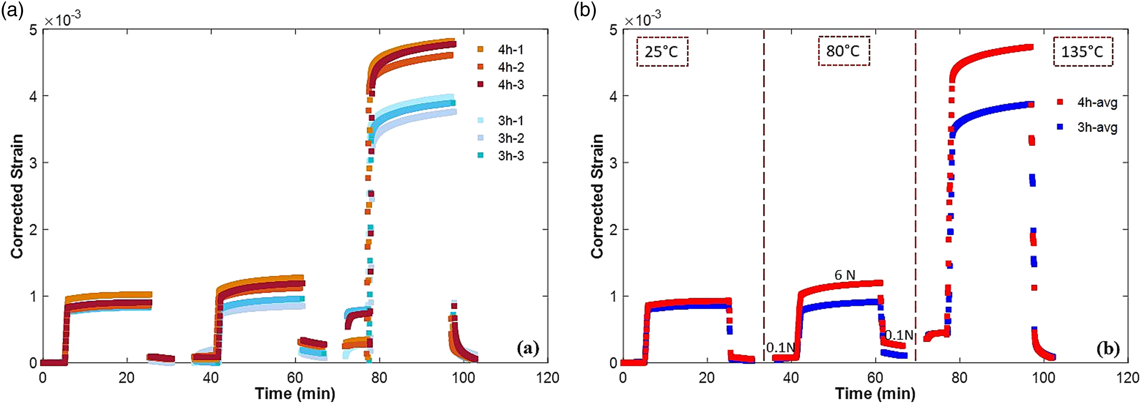

Conclusion

In this work, a thin reusable Skived PTFE sensing film was effectively used to shorten the curing cycle time of a woven CFRP laminate by in-situ cure monitoring using Lamb waves at 70 kHz excitation. Three key cure parameters were looked at to determine the cure stages of the laminate and conclude that the cycle shortening was done successfully, all determined from the velocity and amplitude curves of the recorded A₀ mode: minimum viscosity, full gelation, and vitrification, all occurring after the first soak period which was cut by 1 h. The new 3hr-soak curing cycle was then viably tested for Young’s modulus and tensile strength by doing tensile testing on specimens that were cured at both cycles. The 3hr-soak cycle proved to have superiority in values of both these properties from averaging 10 different specimens for each cycle. To further validate the new cycle enhancement, DMA testing was also used on both cycles in the single cantilever setup. DMA cure findings were similar to both conclusions, as the shift between the cure parameters were also averaged at 1 h, and the final storage modulus recorded slightly higher values for the 3hr-soak cycles. Then, already cured specimens for both cycles were tested in the DMA machine for storage modulus and glass transition temperature. The findings proved better mechanical and thermal properties for the shortened cycle. Finally, DMA was used to test for static fatigue properties in both cycles. Already cured specimens were tested for creep at three temperature scans and the results showed similar performance for both cycles at 25 and 80°C, and better performance for the shortened cycle at T_t of 135°C. Thus, the viability of this cycle shortening was proved. More development can be tested in future work to possibly cut the soaking period by more than 1 h, or to cut down time on different single soak cure cycles.

Footnotes

Acknowledgments

Recognition and gratitude are addressed to the University Research Board at the American University of Beirut and the Lebanese National Council for Scientific Research (CNRS).

Author Contributions

EM: Conceptualization, Formal analysis, Investigation, Writing—Original Draft & Reviewed Manuscript, Visualization. MH: Conceptualization, Validation, Writing—Revision & Editing, Supervision, Funding acquisition.

Declaration of Conflicting Interests

The authors declared no potential conflicts of interest with respect to the research, authorship, and/or publication of this article.

Funding

The authors disclosed receipt of the following financial support for the research, authorship, and/or publication of this article: This work was supported by the University Research Board (URB) at the American University of Beirut grant numbers 103371.

ORCID iD

Elie Mahfoud

References

Mathes

. The composites industry: plenty of opportunities in heterogeneous market. Reinf Plast 2018; 62: 44–51.

Marsh

. Airbus takes on boeing with reinforced plastic A350 XWB. Reinf Plast 2007; 51: 26–29.

Jollivet

Peyrac

Lefebvre

. Damage of composite materials. Proced Eng 2013; 66: 746–758.

Van Grootel

Chang

Wardle

, et al. Manufacturing variability drives significant environmental and economic impact: the case of carbon fiber reinforced polymer composites in the aerospace industry. J Clean Prod 2020; 261: 121087.

Oromiehie

Garbe

Prusty

. Porosity analysis of carbon fibre-reinforced polymer laminates manufactured using automated fibre placement. J Compos Mater 2019; 54: 1217–1231.

Mahfoud

Harb

. Reusable piezo-sandwiched PTFE film for in-process monitoring of advanced composites. J Intell Mater Syst Struct 2021; 32(20): 1045389X2110026. DOI: 10.1177/1045389X211002660

Konstantopoulos

Fauster

Schledjewski

. Monitoring the production of FRP composites: a review of in-line sensing methods. Express Polym Lett 2014; 8: 823–840.

Michel

Ferrier

. Effect of curing temperature conditions on glass transition temperature values of epoxy polymer used for wet lay-up applications. Constr Build Mater 2020; 231: 117206.

Lange

Altmann

Kelly

, et al. Understanding vitrification during cure of epoxy resins using dynamic scanning calorimetry and rheological techniques. Polym 2000; 41: 5949–5955.

10.

Stark

Jaunich

McHugh

. Dynamic mechanical analysis (DMA) of epoxy carbon-fibre prepregs partially cured in a discontinued autoclave analogue process. Polym Test 2015; 41: 140–148.

11.

Hardis

Jessop

JLP

Peters

, et al. Cure kinetics characterization and monitoring of an epoxy resin using DSC, raman spectroscopy, and DEA. Compos A: App Sci Manuf 2013; 49: 100–108.

12.

Kim

Lee

. Dielectric cure monitoring for glass/polyester prepreg composites. Compos Struct 2002; 57: 91–99.

13.

Abraham

McIlhagger

. Glass fibre epoxy composite cure monitoring using parallel plate dielectric analysis in comparison with thermal and mechanical testing techniques. Compos A: App Sci Manuf 1998; 29: 811–819.

14.

McIlhagger

Brown

Hill

. The development of a dielectric system for the on-line cure monitoring of the resin transfer moulding process. Compos A: App Sci Manuf 2000; 31: 1373–1381.

15.

García-Manrique

Marí

Ribes-Greus

, et al. Study of the degree of cure through thermal analysis and raman spectroscopy in composite-forming processes. Materials 2019; 12: 3991.

16.

Aggelis

Paipetis

. Monitoring of resin curing and hardening by ultrasound. Constr Build Mater 2012; 26: 755–760.

17.

Maffezzoli

Quarta

Luprano

, et al. Cure monitoring of epoxy matrices for composites by ultrasonic wave propagation. J Appl Polym Sci 1999; 73: 1969–1977.

18.

Dixon

Jaques

Palmer

, et al. The measurement of shear and compression waves in curing epoxy adhesives using ultrasonic reflection and transmission techniques simultaneously. Meas Sci Technol 2004; 15: 939–947.

19.

Lionetto

Maffezzoli

. Monitoring the cure state of thermosetting resins by ultrasound. Materials 2013; 6: 3783–3804.

20.

Hudson

Yuan

. Automated in-process cure monitoring of composite laminates using a guided wave-based system with high-temperature piezoelectric transducers. J Nondestruct Eval Diagn Progn Eng Syst 2018; 1: 021008.

21.

Mizukami

Ikeda

Ogi

. Measurement of velocity and attenuation of ultrasonic guided wave for real-time estimation of cure-dependent anisotropic viscoelastic properties of carbon fiber-reinforced plastics. Ultrasonics 2019; 99: 105952.

22.

Mizukami

Ikeda

Ogi

. Ultrasonic guided wave technique for monitoring cure-dependent viscoelastic properties of carbon fiber composites with toughened interlaminar layers. Adv Compos Mater 2021; 30: 85–105.

23.

Liu

Zhu

, et al. Cure monitoring and damage identification of CFRP using embedded piezoelectric sensors network. Ultrasonics 2021; 115: 106470.

24.

Kravchenko

Casares

, et al. Digital image correlation measurement of resin chemical and thermal shrinkage after gelation. J Mater Sci 2015; 50: 5244–5252.

25.

Liu

Zhang

Wang

, et al. Effects of cure cycles on void content and mechanical properties of composite laminates. Compos Struct 2006; 73: 303–309.

26.

Pantelelis

Vrouvakis

Spentzas

. Cure cycle design for composite materials using computer simulation and optimisation tools. Forsch Ingenieurwes 2003; 67: 254–262.

27.

Dong

Zhao

, et al. Cure cycle optimization of rapidly cured out-of-autoclave composites. Materials 2018; 11: 421.

28.

Costa

Botelho

Paiva

, et al. Characterization of cure of carbon/epoxy prepreg used in aerospace field. Mater Res 2005; 8: 317–322.

29.

Hernández

Sket

González

, et al. Optimization of curing cycle in carbon fiber-reinforced laminates: Void distribution and mechanical properties. Compos Sci Technol 2013; 85: 73–82.

30.

Hwang

Park

Kwon

, et al. Cure kinetics and viscosity modeling for the optimization of cure cycles in a vacuum-bag-only prepreg process. Int J Adv Manuf Technol 2018; 99: 2743–2753.

31.

Hamdan

Lafi

Hassan

. Optimizing the manufacturing processes of carbon fiber epoxy resin composite panels. J Manuf Sci Eng 2018; 140: 011003.

32.

Frick

Sich

Heinrich

, et al. Relationship between structure and mechanical properties of melt processable PTFE: influence of molecular weight and comonomer content. Macromol Mater Eng 2012; 298: 954–966.

33.

Pernice

De Carvalho

Ratcliffe

, et al. Experimental study on delamination migration in composite laminates. Compos A: App Sci Manuf 2015; 73: 20–34.

34.

Lamb

. On waves in an elastic plate. Proc R Soc Lond Ser A Math Phys Char 1917; 93: 114–128.

35.

Wang

Yuan

. Group velocity and characteristic wave curves of lamb waves in composites: modeling and experiments. Compos Sci Technol 2007; 67: 1370–1384.

36.

Moulin

Assaad

Delebarre

, et al. Modeling of lamb waves generated by integrated transducers in composite plates using a coupled finite element–normal modes expansion method. J Acoust Soc Am 2000; 107: 87–94.

37.

Vázquez

Gosálbez

Bosch

, et al. Comparative study of coupling techniques in lamb wave testing of metallic and cementitious plates. Sensors 2019; 19: 4068.

38.

. Guided lamb waves for identification of damage in composite structures: a review. J Sound Vib 2006; 295: 753–780.

39.

Harb

Yuan

. Impact damage imaging using non-contact ACT/LDV system. Struct Health Monit 2015; 15: 2567–2574.

40.

Harb

Yuan

. Air-coupled nondestructive evaluation dissected. J Nondestr Eval 2018; 37: 50.

41.

Tarraf

Mustapha

Fakih

, et al. Application of ultrasonic waves towards the inspection of similar and dissimilar friction stir welded joints. J Mater Process Technol 2018; 255: 570–583.

42.

Fakih

Tarraf

Mustapha

, et al. Characterization of lamb waves propagation behavior in friction stir welded joints of dissimilar materials. In: IWSHM 2017, Stanford, CA, 12–14 September 2017, pp. 55–62.

43.

Dodson

Inman

. Thermal sensitivity of lamb waves for structural health monitoring applications. Ultrasonics 2013; 53: 677–685.

44.

Feng

Ribeiro

Ramos

. Interaction of lamb waves with the edges of a delamination in CFRP composites and a reference-free localization method for delamination. Measurement 2018; 122: 424–431.

45.

ASTM International . ASTM D 3039/3039M-17: standard test method for tensile properties of polymer matrix composite materials. In: Annual book of ASTM standards. West Conshohocken, PA, American Society for Testing and Materials; 2017.

46.

Ray

Rathore

. Durability and integrity studies of environmentally conditioned interfaces in fibrous polymeric composites: critical concepts and comments. Adv Colloid Interf Sci 2014; 209: 68–83.

47.

Prime

. Dynamic cure analysis of thermosetting polymers. In: Porter

Johnson

(eds) Analytical Calorimetry. Boston, MA: Springer, 1970, pp. 201–210.

48.

Stark

. Investigation of the curing behaviour of carbon fibre epoxy prepreg by dynamic mechanical analysis DMA. Polym Test 2013; 32: 231–239.

49.

Pedrazzoli

Dorigato

Pegoretti

. Monitoring the mechanical behavior under ramp and creep conditions of electrically conductive polymer composites. Compos A: Appl Sci Manuf 2012; 43: 1285–1292.

50.

Chang

F-C

Lam

Kadla

. The effect of temperature on creep behavior of wood-plastic composites. J Reinf Plast Compos 2014; 33: 883–892.