
Abstract
A widely cited study by Osgood and Chambers appeared to extend the generalizability of social disorganization theory to youth violence in rural areas. The results of a very similar study we conducted, however, did not show support for social disorganization, and we concluded that the theory may not be as robust an explanation for rural youth violence as believed. In the current article, we take an important first step in addressing the conflicting findings by examining three likely methodological reasons for the inconsistent results: spatial autocorrelation, sample composition, and measurement of the dependent variable. Multiple tests suggest the first two explanations do not influence the results. Our analyses do indicate, however, that the association between social disorganization and violence in rural areas is sensitive to how the dependent variable is measured. We conclude that scholars should not rely solely on official crime data from rural areas when testing sociological and criminological theories.
Keywords
Introduction
The Federal Bureau of Investigation (FBI, 2009) issued the 2008 Crime in the United States: Preliminary Annual Uniform Crime Report in the summer of 2009. News outlets across the country reported that while violent crimes were decreasing in cities with one million residents or more, small towns with less than 10,000 residents were experiencing increases in violent crimes. While rural crime has received increasing attention in the last decade, it is still an understudied phenomenon. Further, rural areas are sometimes conceptualized as miniature versions of urban areas, with similar social processes occurring at a smaller scale. Others suggest that rural areas are part of a continuum and that there are not only similarities and differences between rural and urban areas but within areas defined as rural as well (Wells & Weisheit, 2004). Until recently, however, hypotheses about rural and urban similarities and differences with respect to crime and its causes have gone untested.
The structural theory that has received the majority of attention in studies of crime in rural areas is social disorganization theory. The handful of studies on this topic relied on arrest data and revealed mixed results, though authors tend to conclude the theory generalizes to rural areas (Barnett & Mencken, 2002; Bouffard & Muftić, 2006; Lee, Maume, & Ousey, 2003; Osgood & Chambers, 2000; Petee & Kowalski, 1993). Unfortunately, these studies all use slightly different measures of social disorganization, different samples, and different measures of dependent variables, so explanations for their inconsistencies are difficult to isolate.
In a recent study, on the other hand, we used the exact same measures of the explanatory variables as Osgood and Chambers (2000), yet relative to the latter come to very different conclusions about the generalizability of social disorganization to rural youth violence (Kaylen & Pridemore, 2011). We suggested three likely methodological reasons for the conflicting results of the two studies 1 : Spatial autocorrelation, sample composition, and measurement of the dependent variable. The goal of this article is to test systematically these three potential explanations for the conflicting results of these two very similar studies of social disorganization and rural youth violence. While the current analysis is specific to these two studies, the nature of the findings will have a broad impact on the growing area of crime in rural areas.
Literature Review
Rural Social Disorganization
Although little empirical research has focused on social disorganization in rural settings, there are theoretical reasons to believe the theory is applicable to rural communities. The concept of social disorganization was popularized by Shaw and McKay’s (1942) analysis of juvenile delinquency across Chicago neighborhoods. While the theory has been refined over time, the general premise remains that communities with high rates of poverty, residential instability, and ethnic heterogeneity are socially disorganized. That is, such communities are more likely to be poorly integrated and thus less able to exert informal social control, properly socialize youth, and solve common problems, thereby resulting in higher rates of crime. The much later work of Sampson (1985) and Sampson and Groves (1989) added family disruption to the list of structural measures of social disorganization.
A variety of literature exists beyond social disorganization theory that links community social and economic change to disorganization in both rural and urban areas. Rapid population growth, ethnic diversity, and the percentage of female-headed households are related to social problems in communities of all sizes (Bacigalupi & Freudenburg, 1983; Freudenburg & Jones, 1991; Guillaume & Wenson, 1980; Rephann, 1999). Research has consistently found links between these factors and crime rates in general (Allan & Steffensmeier, 1989; Crutchfield, 1989; Shihadeh & Ousey, 1998; White, 1999). Major economic changes are also associated with disorganization similarly in urban and rural settings. Deindustrialization and economic restructuring in urban areas and the farm crisis in rural areas similarly led to outmigration of residents, decreased tax bases, increased concentrations of poverty, and weaker social institutions (Bluestone & Harrison, 1982; Ginder, Stone, & Otto, 1985; Wilson, 1996). These similar social effects of economic structural changes in rural and urban areas provide indirect support for the hypothesis that the structural antecedents of social disorganization—residential instability, family disruption, poverty, and ethnic heterogeneity—are similarly associated with social disorganization in urban and rural areas. Whether this corresponding social disorganization is similarly associated with crime in both urban and rural areas remains an empirical question.
For the most part, tests of social disorganization theory in rural settings are said to support the theory. That is, they generally find significant relationships between some of the structural antecedents of social disorganization and crime, with most authors concluding the theory generalizes to rural areas. Specifically, the positive association of crime with residential instability, ethnic heterogeneity, and family disruption is largely consistent in the empirical literature on social disorganization and crime in rural areas (Barnett & Mencken, 2002; Bouffard & Muftić, 2006; Lee et al., 2003; Osgood & Chambers, 2000; Petee & Kowalski, 1993).
Yet while patterns of similarity exist between the rural and urban social disorganization literature, and within the rural literature, researchers have found a number of differences in the relationships between the structural antecedents of social disorganization and violence. These dissimilarities call into question assertions that the theory generalizes to rural areas. These differences include largely conflicting associations between violence and economic measures and a few conflicting findings for the association between violence and racial diversity measures (Barnett &Mencken, 2002; Bouffard & Muftić, 2006; Lee et al., 2003; Osgood & Chambers, 2000; Petee & Kowalski, 1993).
The Kaylen and Pridemore Study
The most widely cited study of social disorganization and crime in rural areas is Osgood and Chambers (2000), the results of which are largely consistent with social disorganization. Given the attention on this article and the carefully documented data and methods employed (see Osgood, 2000), we decided to extend the study using the same measures for the independent variables, sample selection criteria, and methods (Kaylen & Pridemore, 2011). Specifically, we wished to see if the association between social disorganization and crime rates was moderated by population size of the community.
Although we employed a different sample of nonmetropolitan counties, our most substantial departure from the Osgood and Chambers (2000) study was the use of a different measure of the dependent variable (Kaylen & Pridemore, 2011). Osgood and Chambers used youth violent arrest rates as their dependent variables. Subsequent to the Osgood and Chambers (2000) study, however, a series of published studies pointed out serious measurement errors in county-level Uniform Crime Reporting (UCR) arrest data, especially in counties with small populations (Lott & Whitley, 2003; Maltz & Targonski, 2002, 2003). These errors are explained more in depth below. In light of these findings, we employed hospital data on injuries due to assaults among youth and young adults to measure serious violent victimization as the dependent variable (Kaylen & Pridemore, 2011).
As mentioned above, the original intent of our earlier study was to test whether population size moderates the effects of the structural covariates of social disorganization on rural youth violence. However, we found only one measure of social disorganization—single-parent households—to be associated with youth violent victimization, leading us to very different conclusions relative to Osgood and Chambers (2000) about the effects of social disorganization on rural youth violence. We proposed a number of methodological and theoretical explanations for the differences between the two studies. The potential methodological explanations included the presence of spatial autocorrelation (accounted for by us, but not Osgood and Chambers), sample composition (Osgood and Chambers used nonmetropolitan counties from Florida, Georgia, South Carolina, and Nebraska and we used nonmetropolitan counties from Missouri), and measurement of the dependent variable. We carried out extensive tests of the first two explanations and found no evidence to suggest that spatial autocorrelation or sample composition was responsible for the conflicting findings (Kaylen, 2010). Our findings do provide strong evidence, however, that the statistical association between social disorganization and rural youth violence is sensitive to how the dependent variable is measured.
Dependent Variable Measurement
While Osgood and Chambers (2000) used FBI data on youth violent arrests for several types of crime as their dependent variables, we used hospital data on youth violent victimizations as our measure of serious violent victimization (Kaylen & Pridemore, 2011). At the time Osgood and Chambers published their article, there was little research on the validity of arrest data in rural areas. Following their study, however, analyses of these data have shown that a number of serious errors exist at the county level.
Crime data are reported to the FBI by police agencies—or to state agencies who forward the data to the FBI—as part of the UCR Program. Maltz and Targonski (2002, 2003) outline a number of measurement problems that threaten the validity of county-level UCR arrest data. Two of these include missing data and imputation of these missing data. Depending on the data source (i.e., local law enforcement agencies that usually do not impute their data, the FBI, or the National Archive of Criminal Justice Data), the values for any particular county will be different (for more information on imputation procedures, see Maltz & Targonski, 2002).
A third problem with UCR arrest data stems from counties with small populations. Lott and Whitley (2003) emphasized the Maltz and Targonski (2002, p. 313) finding that “smaller counties are more likely to have reporting deficiencies than larger counties.” In some imputation processes, crimes in rural areas are undercounted. For example, when statewide agencies report data at the state level, crime counts are distributed to counties according to their share of the state’s population. In some cases, state agencies operate mostly in rural counties. However, due to imputation decisions, those agencies’ arrests are distributed across all counties. The data for counties with low crime counts, therefore, are severely and systematically affected. For these reasons, Maltz and Targonski conclude that “at this point, county-level crime data cannot be used with any degree of confidence” (2002, p. 316). In fact, they suggest “all studies that use aggregated UCR data—especially at the county level—should be looked at carefully to determine the extent to which coverage gaps and imputations affect their findings” (2002, p. 317). 2
In light of this literature on measurement problems with UCR data, and given the growing number of studies of violence that employ victimization data from hospitals and emergency rooms, we used violent victimization data from hospitals as our measure of youth serious violent victimization in our earlier study (Kaylen & Pridemore, 2011). Hospitals collect data on patients who present to the emergency room. Patients are assigned external cause of injury codes (E-codes) based on the causes of their injuries, including assault (X85–Y09). The Appendix presents a complete list of E-codes used in our analyses. These E-codes are based on the World Health Organization’s (2007) International Classification of Diseases (ICD) codes and are uniform across hospitals. Research has shown these codes to be a reliable source of information about assault injuries treated in hospitals (LeMier, Cummings, & West, 2001) and these type of data are commonly used in studies of violence (e.g., Fabio, Li, Strotmeyer, & Branas, 2004; Fabio, Sauber-Schatz, Barbour, & Li, 2009; Gruenewald, Freisthler, Remer, LaScala, & Treno, 2006). One criticism of using hospital data to gauge patterns of violence is that not all assault victims go to the hospital. This is hardly unique to hospital data, though, and is a common limitation of police data on assault. Of note, May, Hemenway, and Hall (2002) found that offenders—a group thought to be especially unlikely to seek medical treatment—actually do go to the hospital 90% of the time they are seriously injured. Further, hospitals collect patient residency information, so even if a county does not have hospitals, a county can still be assigned a victimization count. For example, if a person living in County A is assaulted and must go to a hospital in County B, the assault will be recorded as an assault for County A due to residency information being collected by the hospital. 3
Given the documented problems with UCR data, we took advantage of the hospital data as an alternative measure of youth violence (Kaylen & Pridemore, 2011). Thus, the differences in the conclusions drawn by the Osgood and Chambers (2000) and us may be attributed to measurement error in the UCR data used by the former and the different measures of youth violence used in these two studies. The purpose of the current study was to address these inconsistent findings. To do this, we examined systematically the crucial question of whether the conflicting results of the two studies are due to differences in the measurement of the dependent variable. If the answer is yes, then this will have broad implications for studying crime and testing sociological and criminological theory in rural areas.
Data and Method
In order to address this question, four data sets were collected and four models estimated. The data sets included (1) hospital victimization data for the Missouri sample (used in our 2011 study), (2) aggravated assault arrest data for the Missouri sample, (3) hospital victimization data for the Florida, Georgia, Nebraska, and South Carolina sample (used by Osgood and Chambers), and (4) aggravated assault arrest data for the multistate sample.
Sample
The same selection criteria used by Osgood and Chambers (2000) and our 2011study were utilized to create the samples. That is, nonmetropolitan counties were selected that have populations of less than 100,000 residents and neither a city of more than 50,000 residents nor more than 50% of their population residing in a metropolitan area of 100,000 or more. The Missouri counties (n = 106) used in the victimization and arrest models are the same as those used in our 2011 study and have total populations ranging in size from 2,382 to 93,807. The multistate arrest model originally used by Osgood and Chambers (2000) is replicated here and consists of nonmetropolitan counties in Florida, Georgia, Nebraska, and South Carolina. This sample of counties (n = 264) has populations ranging in size from 560 to 98,000 residents. Our multistate victimization model has nonmetropolitan counties from Georgia, Nebraska, and South Carolina (n = 197) with populations ranging in size from 444 to 91,582. 4 Florida counties were excluded due to data limitations that are discussed below.
Dependent Variables
Four sets of dependent variable data are used to answer the question of whether measurement of the dependent variable explains differences in the results of the studies by Osgood and Chambers (2000) and us (Kaylen & Pridemore, 2011). The former study used youth violent arrests as their dependent variable while the latter used youth violent victimizations. In order to test the research question, youth violent arrests from the UCR and youth violent victimizations from hospital data were used for each sample. Table 1 provides the descriptive statistics for all dependent and independent variables utilized in addressing the research question. The first row of data for each variable refers to the year 2000 and the second row refers to the year 1990.
Descriptive Statistics for Nonmetropolitan Counties in Five States.
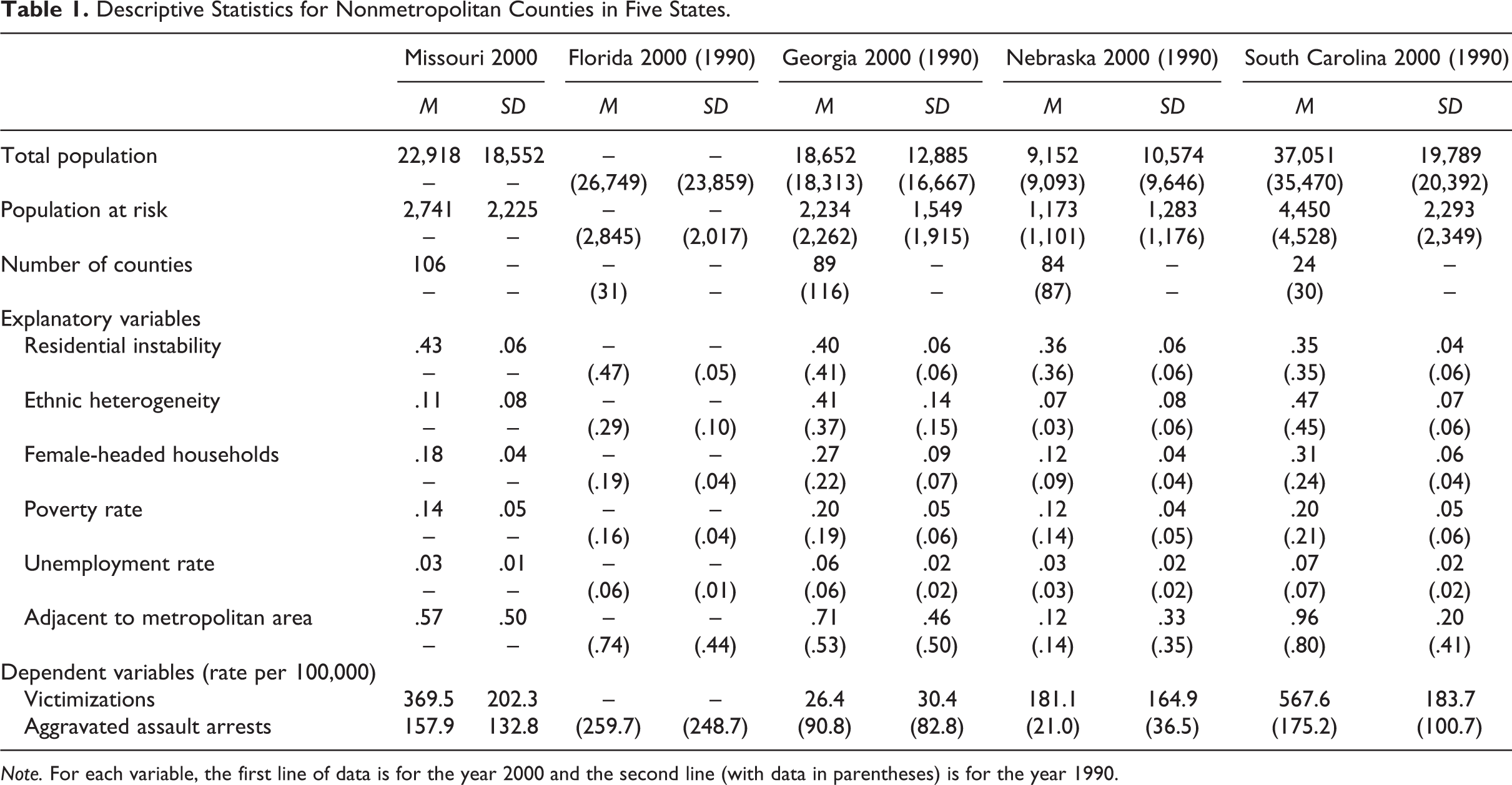
Note. For each variable, the first line of data is for the year 2000 and the second line (with data in parentheses) is for the year 1990.
The youth violent victimization data for Missouri include counts of youth (age 10–17) who were outpatients with injuries coded as assault pooled for the years 1999–2001. As mentioned in the literature review, hospitals collect data on patients who present to the emergency room, including external cause of injury codes and residency information. In all cases, we assigned victims to counties based on residency rather than location of the hospital. These data came from the Missouri Department of Health and Senior Services.
We also collected data on youth arrests in rural Missouri counties. The original study by Osgood and Chambers (2000) employed youth arrest data for eight crime categories. The current study focuses on the aggravated assault category because this most closely mirrors the victimization data employed in our earlier study (Kaylen & Pridemore, 2011). These data include youth (age 10–17) arrests pooled for the years 2001–2003 for aggravated assaults in Missouri.5 The Missouri victimization counts and arrest counts have a significant correlation of .573 (p < .001).
The youth aggravated assault arrest data originally used by Osgood and Chambers (2000) are used in this article for the sample of counties from Florida, Georgia, Nebraska, and South Carolina. The arrest data were provided to the authors by Wayne Osgood and consist of counts of youth (age 11–17) arrests pooled for the years 1989–1993.
The youth violent victimization data for the multistate sample are consistent with those used by us in 2011 and include counts of youth (age 11–17) who were outpatients with injuries coded as assault, pooled for the years 1999–2001.6 Care was taken to ensure similar data were obtained from the Georgia Hospital Association, the Nebraska Department of Health and Human Services, and the South Carolina Office of Research and Statistics. Data were also provided by Florida’s Agency for Health Care Administration. However, these data are reported by hospital location rather than the patient’s county of residence, which is not consistent with our victimization data from the other states. As a result, victimization data were not used for Florida counties.
In order to ensure temporal affects are not accounting for possible differences in the multistate arrest and victimization models, UCR arrest data for Georgia, Nebraska, and South Carolina were collected for the years 1999–2001 and a supplemental analysis was conducted. The arrest and victimization counts for 1999–2001 for the multistate sample have a significant correlation of .697 (p < .001).
Explanatory Variables
The explanatory variables were the same across all models and were consistent with those used by Osgood and Chambers (2000) and us (Kaylen & Pridemore, 2011). These variables are commonly used as measures of the structural antecedents of social disorganization in other studies as well. The variables included residential instability, ethnic heterogeneity, family disruption, and poverty. The Missouri victimization and arrest models and the multistate victimization model used data from the 2000 Census, and the multistate arrest model used data from the 1990 Census (US Census Bureau, 1990, 2000). 7
Residential instability was measured as the proportion of households occupied by people who moved from another dwelling in the preceding 5 years. Ethnic heterogeneity was measured as Lieberson’s (1969) diversity index, which is calculated as
Variable Transformation
The continuous independent variables for the Missouri victimization and arrest models all had positively skewed distributions with skew statistics greater than twice their standard errors. The variables were all transformed by taking their natural logarithms, and since all were substantially less skewed following these transformations, the logged values were used in the analyses. Osgood and Chambers (2000) did not attempt to normalize their continuous explanatory variables that were positively skewed. In the multistate arrest sample, the distributions of residential instability and poverty were both positively skewed with skew statistics greater than twice their standard errors. After transforming their values by taking their natural logarithms, the variables were substantially less skewed and thus the transformed variables were employed in the models. Three of the independent variables—female-headed households, poverty, and unemployment—for the multistate victimization sample were positively skewed, with skew statistics greater than twice their standard errors. Again, these variables were transformed by taking their natural logarithms. The transformed variables were used in the analyses because they were substantially less skewed. 8
Analytic Strategy
Our main research question asks whether the conflicting results of the two studies are due to differences in the measurement of the dependent variable. To address this question, we compare results from the arrest and victimization models within each sample. Consistent results using the same sample (and independent variables) but different measures of the dependent variable would rule out dependent variable measurement as the source of differences between the original two studies. On the other hand, inconsistent results would suggest dependent variable measurement as a likely source of differences between the original two studies.
Following the lead of Osgood and Chambers (2000), we employed the negative binomial estimator in our analyses. Instead of using rates as the dependent variable (as would be done with ordinary least squares regression), counts of the dependent variables were used in negative binomial models. However, as rates are of interest, the models were standardized using the natural logarithm of the size of the population at risk as the offset variable. In addition, dummy variables were also included in the multistate models for all but one of the states to account for any differences between reporting practices in each state. We used SPSS statistics 17 (SPSS Inc., 2009) to carry out the model estimation. In order to test for spatial autocorrelation in the models—something Osgood and Chambers (2000) did not do—global and local tests for spatial autocorrelation of the residuals were conducted. ArcMap 9.3.1 (ESRI, 2009) was used to carry out the spatial analyses separately for each state. Global tests were done using a global Moran’s I statistic (Moran, 1950) with an inverse Euclidean distance spatial weights matrix. Larger values of the statistic indicate greater spatial autocorrelation and thus greater clustering of values by geographical unit. When the global tests revealed spatial autocorrelation was present, the global statistic was decomposed for the model using Anselin’s (1995) local Moran’s I statistic with an inverse Euclidean distance spatial weights matrix. Dummy variables were created to account for clusters of spatial autocorrelation. For each significant cluster, the counties in the cluster were assigned a 1 while all other counties were assigned a 0. These dummy variables were then systematically added to the negative binomial regression model individually and in concert.
Results
Comparison of Missouri Models
Table 2 shows the comparison of the results of the negative binomial models for victimization and aggravated assault arrests for Missouri. It could be argued that if we had originally used arrest data in our 2011 article, there would have been no differences between our findings and those from Osgood and Chambers (2000). In other words, the differential results could be due to our use of a different measure of the dependent variable in our earlier study. However, in comparing the results for victimizations and arrests in Missouri, it is clear this is not the case.
Youth Violent Victimizations and Arrests Regressed on Explanatory Variables With Control for Spatial Autocorrelation; Missouri (n = 106).
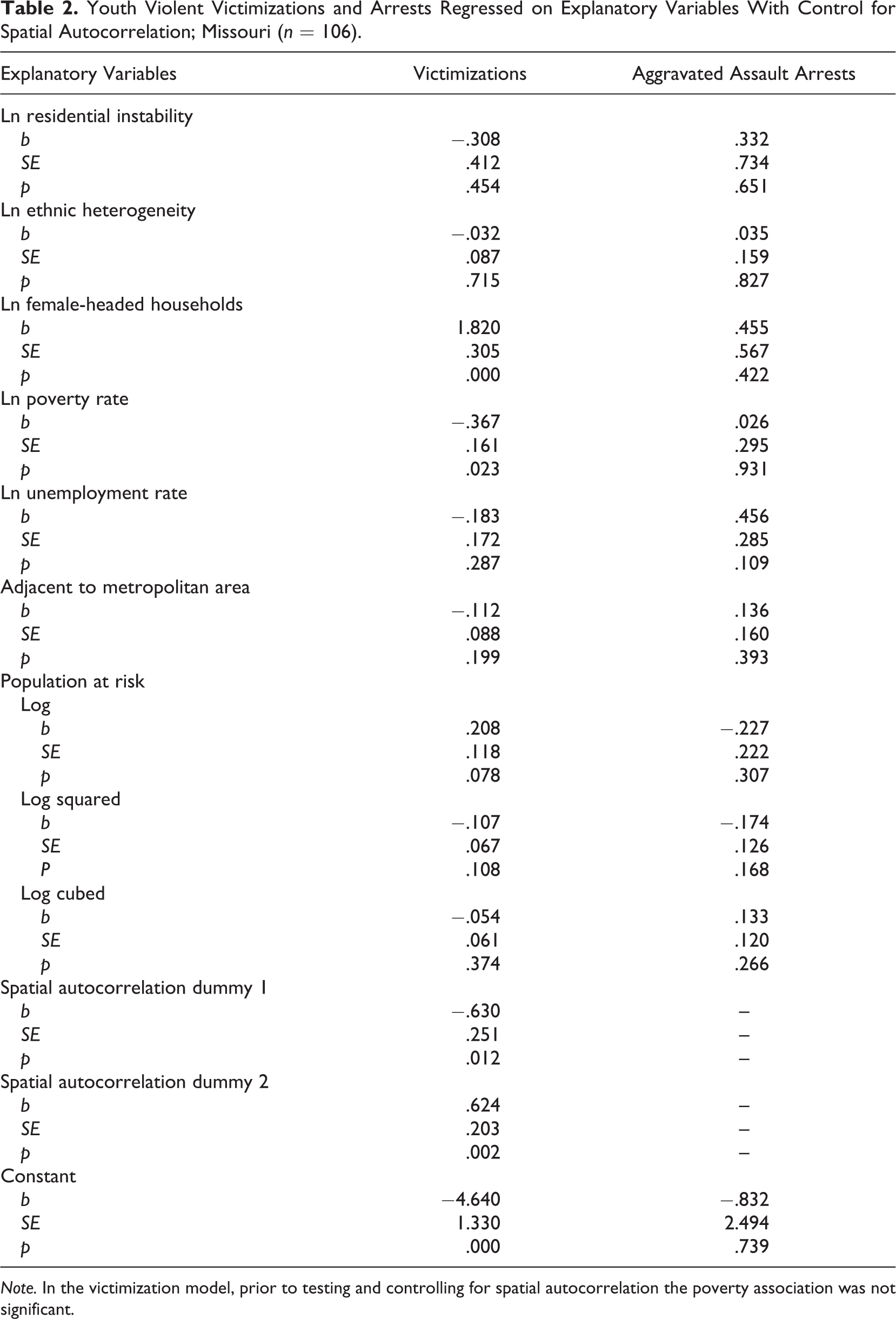
Note. In the victimization model, prior to testing and controlling for spatial autocorrelation the poverty association was not significant.
For the Missouri sample, the inferences drawn from the model employing arrest data are the same as those drawn from the model using victimization data. The results for victimization do not support social disorganization theory in rural areas. Only female-headed households and poverty are significantly associated with youth victimization, with the latter in the negative (unexpected) direction. The remaining social disorganization measures—residential instability and ethnic heterogeneity—are not significantly associated with victimization. The aggravated assault model also does not support social disorganization theory in rural Missouri. None of the measures of social disorganization are significantly associated with aggravated assault arrests.
Common regression sensitivity analyses were conducted for these models along with global and local tests for spatial autocorrelation. The sensitivity analyses revealed no threats to the stability of the models and the inferences drawn. There was evidence of spatial autocorrelation in the victimization models (Moran’s I = .182, p = .006), but not the arrest models (Moran’s I = −.047, p = .566). The local test for spatial autocorrelation in the victimization model revealed two clusters. As shown in Table 2, we have controlled for this spatial autocorrelation.
Comparison of Multistate Models
Table 3 shows the comparison of the results of the negative binomial models for victimization (Georgia, Nebraska, and South Carolina) and aggravated assault arrests (Florida, Georgia, Nebraska, and South Carolina). As discussed above, the Florida counties were excluded from the victimization analyses due to data reporting problems. Furthermore, the arrest and victimization data—and their corresponding explanatory variables—come from different years. The victimization data come from 1999 to 2001 with explanatory variable data coming from the 2000 Census and the arrest data from 1989 to 1993 with explanatory variable data coming from the 1990 Census. Given the different explanatory variables, the variable transformations are not the same for victimization and arrest models. The variables for the victimization model are listed first and the arrest models are listed second.
Youth Violent Victimizations and Arrests Regressed on Explanatory Variables With Control for Spatial Autocorrelation; Florida, Georgia, Nebraska, and South Carolina (n = 264/197).
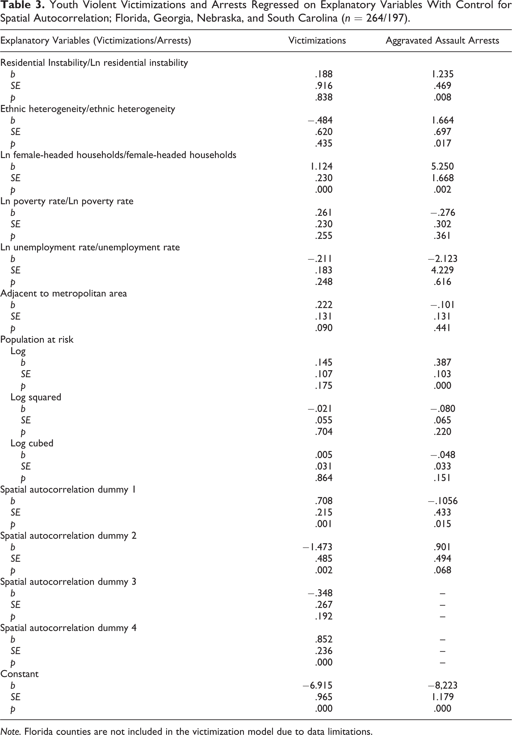
Note. Florida counties are not included in the victimization model due to data limitations.
Comparing the results for victimizations and arrests, it is clear that there are substantial differences in the inferences drawn in relation to social disorganization theory. Consistent with the results from the Missouri models, the results for the victimization model do not support social disorganization theory in rural Georgia, Nebraska, and South Carolina. Of the measures of social disorganization, only the female-headed households association is significant. In comparing these results to the aggravated assault arrest model for Florida, Georgia, Nebraska, and South Carolina, there are considerable differences in the inferences drawn about the applicability of social disorganization theory to rural areas. 9 The arrest model largely supports social disorganization theory with residential instability, ethnic heterogeneity, and female-headed households positively and significantly associated with youth violence. Common regression sensitivity analyses were conducted for the models but revealed no irregularities. There was no evidence of spatial autocorrelation in the global tests for Georgia’s (Moran’s I = .075, p = .090) and South Carolina’s victimization models (Moran’s I = .001. p = .860), but there was for Nebraska’s victimization model (Moran’s I = .187, p = .001). The local test for spatial autocorrelation in Nebraska revealed four clusters. In the arrest models, global tests revealed spatial autocorrelation in Florida (Moran’s I = .343, p = .019) but not Georgia (Moran’s I = −.065, p = .332), Nebraska (Moran’s I = .606), or South Carolina (Moran’s I = −.041, p = .973). The local test for spatial autocorrelation in Florida revealed two clusters. In instances in which spatial autocorrelation was present, it was accounted for in the models as shown in Table 3.
Supplemental Analysis
An additional analysis was conducted in order to ensure there was not a temporal cause for the differences in the multistate arrest and victimization models. UCR arrest data for Georgia, Nebraska, and South Carolina were collected for the years 1999–2001 to be consistent with the victimization model. 10 UCR arrest data were not available for Florida during this time. As such, the multistate arrest and victimization samples and independent variables for 2000 are identical. Table 4 shows the results of this model. Overall, the model is fairly consistent with the multistate arrest model from 1990. That is, the results generally support the generalizability of social disorganization to rural areas.
Youth Arrests Regressed on Explanatory Variables; Georgia, Nebraska, and South Carolina (n = 197).
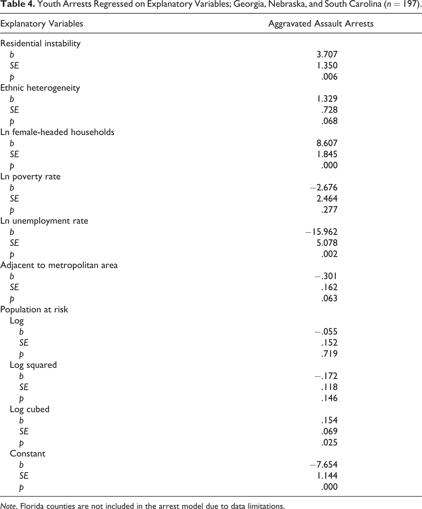
Note. Florida counties are not included in the arrest model due to data limitations.
In short, based on the comparisons shown here we conclude that the different inferences drawn by Osgood and Chambers (2000) and us were very likely due to measurement of the dependent variable (Kaylen & Pridemore, 2011). When using exactly the same units of analysis, samples, years, and explanatory variables in two samples (Missouri and the three-state sample), the conclusions are the same: Inferences are different when using hospital victimization data and UCR arrest data. While there are minor differences in the multistate arrest models between the years centered on 1990 (the years of Osgood and Chambers’ study) and the years centered on 2000 (our supplemental analysis), the conclusions remain the same.
Discussion
Our 2011 study questioned the strong conclusion many have drawn, mostly based on Osgood and Chambers’ (2000) findings, that social disorganization theory generalizes to youth violence in rural areas. We highlighted a number of methodological and theoretical questions about the differences between the two studies and the generally inconsistent findings from the empirical literature on social disorganization and rural crime thus far. The purpose of this article was to address the question of whether the differences in the studies by Osgood and Chambers and us were due to common methodological problems (Kaylen & Pridemore, 2011). After ruling out spatial autocorrelation (it does not affect the results) and sample composition (the general conclusions are the same in both samples), our results point to dependent variable measurement as the most likely reason for the differing conclusions. This finding is consistent with similar research on and conclusions drawn about differences in homicide estimates from various sources and the impact this can have on hypothesis tests (Wiersema, Loftin, & McDowall, 2000), and our results have important implications for the study of crime and tests of social disorganization in rural areas.
Measurement Error in the Dependent Variable
Given the measurement errors in county-level UCR arrest data (Lott & Whitley, 2003; Maltz & Targonski, 2002, 2003) that came to light subsequent to the Osgood and Chambers (2000) study, it is not surprising that an alternative measure of youth violence would yield conflicting results. It is important to note that the UCR was never intended to provide crime estimates at the county level, but rather the program was created to provide annual national estimates of crime levels (Lynch & Jarvis, 2008). Even within the first year of publication of UCR data, critiques came out about using the data for comparative purposes across jurisdictions (Sellin, 1931; Warner, 1931). If there are problems with nonreporting, undercounting, and imputation of arrests in counties with small populations, but similar problems do not exist with hospital victimization data, then regression results for each data source might be different. When measurement errors in the dependent variable are not random, the slope coefficient is biased. Even when these errors are random, the standard errors are larger. Further, differences in counts from the UCR arrest data and the hospital data will likely lead to different inferences being drawn about relationships. Wiersema et al. (2000) have come to similar conclusions about measuring homicide, including the differential effects on the inferences drawn when studying smaller counties.
Research has shown that counties with smaller populations have larger measurement errors (Lott & Whitely, 2003; Maltz & Targonski, 2002, 2003), and the effects of these errors are likely compounded when testing social disorganization in rural areas. Measurement errors in county-level arrest data for youth assaults might be systematically related to the size and social organization of the community. In smaller communities, for example, greater social cohesion might make arrest less likely when a crime occurs. Donnermeyer and colleagues (Barclay, Donnermeyer, & Jobes, 2004; Donnermeyer & Barclay, 2005) found that in rural areas arrest decisions are often based on fear of disrupting community cohesion. These crimes are either not reported to the police or the police do not follow up with reports because of this fear. Likewise, Weisheit, Falcone, and Wells (2006) reported that the likelihood that a violent crime is reported to the police is lower in rural areas because rural violence typically occurs between acquaintances and because there is a general distrust of government in rural areas. One study found that in a rural community, residents were unlikely to call the police in cases of abuse because the police and prosecutor were reluctant to act (Gagne, 1992).When crimes occur and an arrest is not made for these types of reasons, which are closely associated with social organization, the slope coefficient is biased in the same direction as the hypothesized association. In other words, the hypothesis drawn from theory is that as social organization increases youth violence decreases. Yet this prior research suggests that as social organization increases the likelihood of reporting the crime to the police and the police making an arrest also decrease. This bias in the estimate could result in finding a significant association (in favor of the theory) where none actually exists, thus making support for the theory an artifact of measurement.
Do Arrest and Hospital Data Measure Different Things?
It could be argued that differences exist between arrest and hospital data because they measure different things. Arrest data measure a mixture of offending behavior, whether the victim reports to the police, and police investigation and arrest practices. Hospital data measure victimization and whether the victim presents to the hospital. Although youth offending and victimization are not the exact same thing, Boney-McCoy and Finkelhor (1995) found that most nonfamily aggravated assaults against youth aged 10–16 were committed by peers within 3 years of the age of the victim. Bursik (1988) suggests the effects of social disorganization variables may be crime-specific. In disentangling Bursik’s (1988) idea and the notion of social disorganization versus organization, Roussell, Holmes, and Anderson-Sprecher (2009) distinguish between behavior grounded in interpersonal conflict (e.g., youth violence) and behavior grounded in interpersonal cooperation (e.g., methamphetamine use). If social disorganization theory is supposed to explain behavior grounded in interpersonal conflict (as the authors suggest), the theory would operate similarly in regard to youth offending and victimization. Furthermore, it would operate similarly in regard to these two types of youth violence regardless of whether the youth are offending or being victimized by each other. Bursik (1988) also supports this notion in his theoretical connection between victimization and social disorganization. Consistent with routine activities theory (Felson & Cohen, 1980), he suggests community disorganization represents the ability of the community to supervise the actions of offenders and opportunities. When offenders and opportunities meet unsupervised, victimization occurs. Therefore, it seems plausible that social disorganization theory would operate similarly with regard to youth violent offending and violent victimization. In fact, several key social disorganization theory studies have utilized self-report victimization data including the classic study by Sampson and Groves (1989).
The hospital data used to measure youth serious assault victimizations and the youth aggravated assault arrest data are consistent in theory but may not be consistent in practice. As discussed above, social disorganization theory should operate similarly with regard to both types of youth violence. Our focus on serious assaults minimizes the risk that hospital and aggravated assault arrest data are measuring different things. Violent crimes such as robbery do not have a reliable alternative indicator to arrest data, but serious assaults do. Hospitals have specific injury classifications for assaults based on the World Health Organization’s (2007) ICD codes that are employed uniformly across hospitals. Research has found these intent of injury codes to be accurately assigned as assaults over 90% of the time (LeMier et al., 2001). Furthermore, assault victims are likely to seek medical treatment. Even criminals, a group thought unlikely to go to the hospital, go 90% of the time they are seriously injured (May et al., 2002). The relatively low correlations between the two data sources are consistent with those found by Wiersema et al. (2000) in homicide data. They also concluded that different inference can be drawn when using two data sources that measure the same thing yet have low correlations. Therefore, it appears that different sources of data on youth violence result in different inferences being drawn not because they measure different things but because of differences in their measurement errors.
Rural Social Disorganization
The current study sought to examine potential methodological explanations for the prior inconsistencies in the rural social disorganization and crime empirical literature. However, there may also be important theoretical considerations to take into account. Social disorganization theory might be purely an urban theory of crime and not applicable to rural areas. If this is the case, theoretical explanations for the inapplicability should be explored and a rural theory of community crime rates should be constructed. We proposed several theoretical possibilities in our earlier article and the theoretical and empirical literatures provide a number of plausible reasons why social disorganization theory may not be associated with rural crime (Kaylen & Pridemore, 2011).
Structural Antecedents of Social Disorganization
Both the nature of social structure in rural communities and the impact of social structure on social relations in rural communities may be different than in urban communities. Social disorganization theory posits that the structural antecedents of social disorganization affect crime by increasing community social disorganization in the form of social cohesion and mutual trust. However, social structure might affect social disorganization differently in rural areas.
It may be that the community social disorganization explains differences in crime rates in rural areas but that this disorganization is preceded by different structural factors in rural versus urban communities. For example, the spatial composition of the community may affect social disorganization. A rural farming community where the nearest neighbor is a considerable distance away may not be as cohesive as a rural, small town community in which people live near each other. Furthermore, a rural community in which residents go to work, school, and church together may be more cohesive than a rural community in which residents commute to towns or cities for these activities. While Weisheit et al. (2006) suggest social life in rural communities revolves around social institutions, some rural communities may turn elsewhere for these social institutions and thus have different levels of social organization. Future research on social indicators of crime in rural communities should consider that different types of rural communities exist with distinctions beyond adjacency to metropolitan areas.
Osgood and Chambers (2000) allude to the possibility of the structural antecedents of social disorganization operating differently in rural and urban areas. They emphasize the strength and consistency of the family disruption measure (female-headed households) in rural studies, which also holds for both victimization models presented in this article. It may be that in rural communities, social disorganization is related more to family factors than to residential instability and racial/ethnic composition. Osgood and Chambers touch on the notion that residential instability may not operate similarly in rural and urban areas. They suggest that “outside the metropolis, populations of poorer communities may be more stable than average, not less” (Osgood & Chambers, 2000, p. 106). Barnett and Mencken (2002) also point out this rural poverty–stability finding. The rural poor might not face the same housing pressures as the urban poor and thus may be able to maintain more stable housing (Roussell et al., 2009). Literature on farm job loss mirrors this sentiment. Residents did not move out of rural communities at the same levels as occurred with deindustrialization in urban communities (Ginder et al., 1985). Future research should aim to identify the structural antecedents of community social disorganization in rural areas, perhaps using female-headed households as a starting point.
The problem of model misspecification may conceal the complex social structure and social disorganization relationships discussed above. A properly specified social disorganization model should test a mediating model where social structural factors influence the level of community social organization, which in turn affects crime rates. Such a model, however, has yet to be tested in the rural literature due to the lack of data on the mediating processes. The results of our study show that the common structural antecedents used in urban studies do not predict youth violence similarly in rural areas (i.e., there is not a direct effect). It is unknown what affect those structural antecedents have on rural social organization, though, because measures are not commonly available and thus are not included in any studies to date of social disorganization and crime in rural areas (Kaylen & Pridemore, 2011).
Social Organization
There may also be differences in the nature of social relations and crime in rural and urban communities. Donnermeyer (2006) points out that some forms of community organization in rural areas may actually facilitate crime, so social disorganization theory may not be applicable. Donnermeyer and his colleagues (Barclay et al., 2004; Donnermeyer & Barclay, 2005) found that in rural Australia, livestock theft is often not reported to the police or police do not follow up on complaints because of a fear of disrupting community cohesion. Thus, not only does social organization appear to be associated with decreased crime intervention, but it also appears to be associated with errors in the measurement of crime as discussed above. If the police are not investigating crimes, arrests are not made and the crimes are not counted. Therefore, some communities with high levels of social organization might appear to have lower crime rates than they actually have, and the reason for this lies precisely in their level of organization, at least as indicated by traditional measures. Likewise, DeKeseredy and colleagues (DeKeseredy & Schwartz, 2009; DeKeseredy, Schwartz, Fagin, & Hall, 2006) found that community organization in rural areas can actually support violence against women. Men in these communities share stories and techniques about violence with each other in public places and support for this violence has become a part of the mainstream culture. Furthermore, Roussell et al. (2009) concluded, consistent with Bursik’s (1988) idea that social disorganization applies to only some types of crimes, that traditional structural measures of social disorganization theory did not predict rural methamphetamine use because this type of drug use is more associated with social organization. Thus, rather than community organization inhibiting certain types of crime in rural communities, it might actually facilitate it or lead to measurement errors.
Conclusion
The goal of this study was to explain the conflicting results of two very similar studies of rural social disorganization and youth violence. The results of the negative binomial models indicated that measurement of the dependent variable is the most likely methodological explanation of the different inferences drawn by Osgood and Chambers (2000) and us (Kaylen & Pridemore, 2011). The former study used arrest data to measure youth violent offending while the latter used hospital data to measure youth violent assaultive victimization. We used an alternative measure of the dependent variable in our 2011 study because empirical evidence came out subsequent to the Osgood and Chambers (2000) study that questioned the reliability of county-level UCR arrest data, especially in counties with smaller populations (Kaylen & Pridemore, 2011). When we reestimated the model, we used in our 2011 study with arrest data, the results were the same as our original model that used victimization data. However, when we reestimated the Osgood and Chambers (2000) model with victimization data, the inferences drawn were different than their original model that used arrest data.
While methodological questions are critical to theoretical literature, the original intent of the Osgood and Chambers (2000) study should not be forgotten. The authors sought to test the generalizability of social disorganization theory to rural youth violence. The current study does not support this generalizability, as the theory is currently tested, in rural areas. Until a test of the full systemic model of social disorganization is carried out, strong conclusions about the generalizability of the theory to rural crime and violence should not be made.
Our goal was not to argue that one of the two conflicting studies was better than the other or to question the careful work done in both articles. Instead, the aim was to address important methodological questions about why the differences occurred, because the answers to these questions go well beyond the two original studies and have important ramifications for the study of crime in rural areas more generally. Furthermore, the conclusion that measurement of the dependent variable is the cause of the differences in the original two studies is not an indication that hospital violent victimization data are without limitations and should necessarily be used in place of arrest data in all studies. Rather, the hope is that the results of this article will spur more critical evaluation of measures of dependent variables in criminological research. As demonstrated in this article, the data one uses can greatly impact the inferences drawn about the efficacy of theoretical explanations. Until problems with county-level UCR data are adequately addressed, alternative measures should be explored. The literature on measurement of crime and violence should be brought into the forefront of the empirical literature on theory testing and, as demonstrated here, replication studies should be performed to strengthen our confidence in the robustness of results.
Footnotes
Appendix
Acknowledgment
We thank Richard Spano and Arvind Verma for their helpful critiques of earlier versions of this article and Wayne Osgood for his guidance and for providing access to his original data. We also thank the Georgia Hospital Association, the Missouri Department of Health and Senior Services, the Nebraska Department of Health and Human Services and its medical record and health information registries, and the South Carolina Office of Research and Statistics for providing us with hospital data.
Declaration of Conflicting Interests
The author(s) declared no potential conflicts of interest with respect to the research, authorship, and/or publication of this article.
Funding
The author(s) received no financial support for the research, authorship, and/or publication of this article.