Modelling waste generated during construction of buildings using regression analysis

Abstract

The building industry is responsible for a large amount of waste, and the measurement and modelling of this waste could be used to develop better waste management plans. Several theoretical models explain the relationships between waste and building characteristics, but local practices may result in different behaviours. This study aimed to measure and analyse the waste generated through construction. It was based on the analysis of 18 building sites located in the region of Porto Alegre, Brazil. Waste was measured at these sites, and the results showed an average waste generation rate of 0.151 m³ m^-2. A regression analysis of the collected data presented a satisfactory performance in two models. The first model was developed to explain total waste generation, including the effects of certain attributes, with an R² = 0.81. The changes in waste generated during construction were estimated. The second model considered time schedules and examined the effect of the construction stage on waste generation, and reached an R² = 0.91. The model with time indicated an S-shaped relationship. The models presented satisfactory statistical parameters and could be used to produce better waste management plans in the preconstruction stage.

Keywords

Construction industry waste generated waste modelling construction stage buildings preconstruction

Introduction

A substantial share of extracted raw materials and energy is used for the production and transport of materials and components in the construction industry. The industry also generates a large amount of waste (Roaf et al., 2012; Yang et al., 2017). Construction and demolition waste (C&D waste) is an important problem in environmental management, and in order to solve this problem actions should be taken to reduce waste generation, increase reuse and recycling, and ensure proper disposal, as a significant portion of waste is deposited at unauthorised waste disposal sites (Bakshan et al., 2017; Magalhães et al., 2016; Menegaki and Damigos, 2018; Paz et al., 2018; Ram and Kalidindi, 2017). It is common to verify the absence or weakness of waste management plans in the construction industry (Ajayi et al., 2017; Bakshan et al., 2017; Cooke and Williams, 2014; Villoria Sáez and Osmani, 2019). One plausible reason for this environmental management problem is the lack of organised information about C&D waste generation, at a municipal scale and a site scale. Information on C&D waste generation at the municipal scale could improve public waste management, while it could allow for the development of better building management plans at the site scale. In both cases, it is important to increase the knowledge concerning the types and quantities of waste generated in the building sector (Bossink and Brouwers, 1996; Gangolells et al., 2014; Wu et al., 2014).

Some countries have public data collections on C&D waste, such as that available in China and Hong Kong. Chen and Lu (2017), Lu et al. (2016), Song et al. (2017), and Wu et al. (2016) used organised data records to study waste generation in these countries. It is not the case in Brazil. As occurs in other countries, there are few initiatives on public measurement, and Brazil does not have enough information available on waste and building characteristics to allow for developing models (Alfaia et al., 2017; Medina Jimenez et al., 2019; Penteado and Rosado, 2016). In this sense, according to Ram and Kalidindi (2017), it is important to generate consistent estimates of C&D waste in regions with limited data availability. Moreover, there are a few other C&D waste estimation studies, including one that focuses on the time when the waste is generated during the construction stage.

The research gap addressed in this study is the development of models that can be used in the preconstruction phase to forecast waste generation. This study aims to analyse the waste generated during construction. It presents two models, based on regression analysis, designed to estimate the waste generated and analyse the influence of building attributes and development schedule on the waste rate.

Literature review

General studies are available for use in public planning. These works are designed to obtain estimates at a municipal or country scale. Other efforts are concentrated on the evaluation of building projects, at a construction site scale, and these studies aim to help practitioners in the construction industry to develop on-site waste management plans.

At a larger level, some studies have been presented. Wu et al. (2015) developed a model to estimate waste generation at a municipal level based on gene expression programming (GEP). They collected a sample of municipal waste collected, with two decades of quarterly data, and used some factors as predictor attributes. The model reached an R² = 0.82 and the error of the GEP model was lower than in linear regression and artificial neural network (ANN) studies. After Wu et al. (2016), the C&D waste generated in the renewal of large cities in China can achieve billions of tonnes. An amount of 14 million tonnes of waste generated by year was estimated to the city of Shenzhen. They estimate a potential gain on recycling greater than 1 billion USD. Ram and Kalidindi (2017) studied the case of Chennai city, India, using regression models and estimated more than 1.1 million tonnes of waste generated in the city in 2013. Song et al. (2017) presented a model to estimate the amount of waste generation by region in China. They forecast the generation of waste in 2018 as around 196 million tonnes from construction waste and 192 million tonnes from demolition waste around the country. Jain et al. (2018) made estimations to C&D waste under some scenarios to India, calculating an average of 289 million tonnes of construction waste in view of 2016 data. Using data from 17 countries, Menegaki and Damigos (2018) developed a regression model relating C&D waste per capita with construction gross domestic product (GDP), GDP per capita, and population density. Kupusamy et al. (2019) calculated an amount of 601 thousand tonnes of C&D waste to the peninsular of Malaysia, in figures to 2016, calculating parcels for each region. In the same way, Zhang et al. (2019) estimate a generation of 4.1 billion tonnes of C&D waste, also to 2016 in China.

In contrast, waste measurement at the building site scale can be addressed in various ways by obtaining measures or estimates of the waste generated and by developing models to preview it. Wu et al. (2014) presented a review of the literature on construction waste measurement. They examined 57 scientific articles and classified these studies according to three research criteria: Waste generation activities, proposed quantification methods, and estimated waste quantities. Estimation methodologies can be further categorised according to the use of direct or indirect measurements. Direct measurement is performed by measuring waste at the building site. Indirect estimation is often based on either the number of trucks or containers used for the removal of waste or based on the estimations made in the budgets. The waste estimation analysis may include all the materials found on site or a choice of the most important ones, in terms of quantity or cost.

The data measurements made at building sites are valuable. Among the first waste measurement studies was that of Skoyles and Skoyles (1987). They used measurements from 114 buildings, considering 22 materials, and found a general rate of 10% of loss in materials (as a percentage of the total mass), nearly twice the rate calculated in conventional budgets. Bossink and Brouwers (1996) and Hao et al. (2008) developed similar studies and found a level of losses ranging from 1% to 10% of the volume of material bought.

Several authors developed quantitative studies of waste measurement at working sites. Table 1 shows waste generation rates in distinct locations based on a number of different studies. Some studies indicate the waste rate in volume by built-up area (m³ m^-2), while others use a relation of mass by built-up area (kg m^-2). Ranges of 0.031 to 0.201 m³ m^-2 and 38 to 150 kg m^-2, respectively, could be verified. In case of retrofit, however, there are few studies. Villoria Sáez et al. (2018) presented two cases of vertical envelope changes, with waste figures of 0.008 to 0.012 m³ m^-2 and 2.46 to 65.24 kg m^-2, in different conditions.

Table 1.

Waste generation rates in distinct locations.

Location	m³ m^-2	kg m^-2	Type of construction project	Source
Australia	0.084		Non-residential	McDonald and Smithers (1998)
Bangladesh		64	Residential and non-residential buildings	Islam et al. (2019)
Brazil	0.069–0.200	50–150	Residential and non-residential buildings	Soibelman (1993), Pinto (1999), Formoso et al. (2002), Sardá (2003), Souza et al. (2004), Marques (2007), Oliveira (2008), Brönstrup (2010), Kern et al. (2015), Lafayette et al. (2018)
China		41-55	Residential buildings	Li et al. (2013); Liu et al. (2018)
European Union		44–115	Residential buildings	Mália et al. (2011)
Hong Kong	0.175		Residential and non-residential buildings	Poon et al. (2001)
India		66	Residential buildings	Vilventhan et al. (2019)
Israel	0.201		Residential buildings	Katz and Baum (2011)
Lebanon		38–43	Residential buildings	Bakshan et al. (2015)
Spain	0.031–0.192		Residential buildings	Solís-Guzmán et al. (2009), Villoria Sáez et al. (2012), (2014), (2015)
United States		69	Educational building	Backchan and Faust (2019)

It is also possible to adopt an estimate based on documentation, using a budget supported on a work breakdown structure, bill of quantities, or material purchase lists. In this case, the loss rates considered in the budget are taken into account. Villoria Sáez et al. (2012) presented a study of waste calculation using a cost database obtained from the Catalonian Institute of Technology (ITeC, 2012), Spain. Li et al. (2016) proposed a model to estimate waste using a work breakdown structure based on building design. The model could estimate waste and identify its origin, type, packaging, and other characteristics. In recent years, some authors, such as Akinade et al. (2018), Guerra et al. (2019), Kim et al. (2017), and Mercader-Moyano et al. (2017), have developed and continue to develop models supported on building information modelling (BIM) to estimate waste generation based on building design. Akinade et al. (2018) used BIM and neural networks to generate a model that could integrate into Autodesk Revit as an add-in component. This author used data from 117 buildings and concluded that waste forecastin the design stage could improve construction decisions and allow the project team to make better choices. Kim et al. (2017) used quantity lists incorporated to a BIM platform to estimate the amount and type of waste in a building project. Mercader-Moyano et al. (2017) used BIM combined with the cost database of Andalucía (Spain) to calculate steel and concrete waste. Guerra et al. (2019) provided a study based on automatic measurements on BIM comparing them with purchasing records on an educational building, specifically to concrete and drywall. This approach obtains an estimate of the generated waste, which is useful in the preconstruction phase. However, BIM does not provide reasons for the results and cannot be used to estimate wastes in other projects.

The third way to analyse waste is through the development of models. Based on building information, developing models of the design and construction processes can help to understand why construction waste is generated, and this allows for a more detailed analysis than a simple estimation of waste generation rate. There are several studies conducted on waste modelling using regression analysis and artificial intelligence models.

Villoria Sáez et al. (2014) analysed seven building projects, measuring volume and weight of wastes at building sites. They included the time dimension using a term called the ‘normalised project duration’, which related the percentage of waste generated with the corresponding percentage of time passed. Using this scale, waste progressively accumulates at the site until the total measured amount is reached. The study indicated an S-shaped relationship between time and waste or time and waste generation rate. The authors proposed regression models relating time and waste generation rate in two ways, by volume and by weight. The models presented were in cubic form (including time, time², and time³ components). The coefficients of determination, greater than R² = 0.97 in both models, and other presented statistics indicated satisfactory model behaviour. Furthermore, the models had no intercept term, which is coherent with the shape of the curves obtained using the observed values of waste.

Kern et al. (2015) studied 18 high-rise building projects and developed a model based on various design attributes. The proposed model was linear and demonstrated satisfactory statistical performance (coefficient of determination of 0.694 and all attributes approved on t-tests at the 5% level). The model indicated the relationship between waste and several attributes, such as floor size (in m²) and ratio of the number of residential floors to the total number of floors (including service and parking levels). Another remarkable attribute indicated if the waste was reusable on the same building site.

Villoria Sáez et al. (2015) proposed two models considering floor size and number of houses. They selected eight projects and measured the waste generated at their sites. The first model estimated the amount of waste in mass, and the second one calculated it as a volume. Both models reached a coefficient of determination of R² = 0.998, adopting a 5% significance level for the attributes. Estimations based on the model presented a mean deviation of 10% compared with the measured values. The model included a correcting factor, based on the number of house units and the built-up area. This factor appeared in the linear, quadratic, and cubic forms of the model.

Several other techniques, besides regression, have also been used to develop models. Lee et al. (2016) developed a hybrid model to estimate the amount and cost of waste at the preliminary stages of a project. The proposed model used an ANN and ant colony optimisation (ACO), using information on 118 multifamily residential buildings in South Korea. The authors divided the buildings into two categories by using 113 cases to build the model and 15 cases to test it. The attributes used were location, number of stories, number of buildings, number of units, completion and demolition years, number of houses, plot area, and gross floor area. The output studied was concrete waste (in tonnes). The models achieved less than 18% of mean absolute error rate on an estimation based on neural networks and 14% on the hybrid model using an ANN and ACO. Liu et al. (2018) developed a model using ANN and a particle swarm optimisation algorithm to avoid problems with a back-propagation learning scheme. They tested with 20 cases of residential buildings in Shangai and found a model with less than 12% of error rate.

Lu et al. (2016) proposed a model based on S-curves to estimate waste generation. After examining several functional forms, the model was developed using waste generation measures and certain project characteristics (such as total budget, location, and duration of construction), with standardised scales of time and waste generated, which were adopted to compensate the effect of different project sizes. The model was developed using more than 37,000 records collected in Hong Kong through an ANN. The model used a scheme combining genetic algorithms with a back-propagation mechanism to obtain the ANN weights. The form of the final model equation was a cumulative logistic distribution.

The analysis of these studies reveals several findings. Some studies use a small number of samples (less than 30 cases). Most studies use the floor size and number of floors in their models, while the building schedule is not always included explicitly. Models that do not take into account time can be considered stationary because they do not consider the timeline of waste generation in the building construction process. However, models including time can be denominated as dynamic as they consider the change in waste generation rate with the schedule. Furthermore, the models give good insight into the expected S-shaped relationship between waste generated and time.

Moreover, these studies used different techniques to develop the waste estimation models, including regression analysis, ANN, and genetic algorithms. While ANN applications provide high accuracy, the models are not explicit. This makes it difficult to understand the main causes of waste generation. In contrast, regression models present coefficients or weights and can analyse the individual significance of each factor, which can result in more specific planning in the preconstruction phase.

Materials and methods

Waste measurement

An empirical study was developed to obtain information on local projects. The first step involved measuring waste at building sites. There were no public statistics or measurements available on the selected region. Construction projects were sampled, materials used were identified, and waste management programmes (mandatory as per Brazilian environmental agencies) and construction schedules were analysed. Soil movement and foundation work were not taken into consideration because they could differ with building sites. Notwithstanding, care was taken to ensure that the first waste collection measurements were not based on the debris left behind by the preceding stages of work. All building sites considered in this study followed strict control as waste was collected daily. The waste containers were always collected by the same employees at each construction site to preserve metrics. Construction sites in Brazil usually collect waste in 4 to 5 m³ metallic containers that are strategically scattered throughout the site; when such containers are full, garbage trucks move them to municipal disposal facilities. No waste was stored at the construction site for more than one and a half days. Therefore, small distortions regarding the time of waste measurement could be expected.

On-site measurements and design attributes

The study included 18 building construction sites in the town of Porto Alegre, southern Brazil. The structural systems consisted of reinforced concrete structures, masonry walls, and other conventional structural systems. According to the author’s experience and knowledge on building practices, these projects could be considered as standard building projects. Visits to the sites were carried out on a regular basis (weekly or bi-weekly) to collect waste generation data and to examine other characteristics during various construction phases. Table 2 identifies the observed characteristics of these projects. The meaning of each attribute presented in the table is as follows.

Type of building (Type): Classifies the building: 1 = apartment building; 2 = mixed tower (apartments and offices); 3 = office building.

Floor size (FLS): Denotes the total built-up area, measured in square metres (m²).

Number of floors (NFL): Number of stories.

Number of dwellings (DWE): Number of individual units in the building (apartments or offices).

Quality management on site (QUA): Level of quality management verified on-site, classified by the researcher’s observation in three levels: 1 = there is an active quality management system based on ISO 9000; 2 = there is an ISO 9000-based system, but it is partially followed; 3 = there is no quality management.

Reuse or recycling of waste on site (REC): Level of reuse or recycling applied to building waste on-site, categorised by the researcher’s observation in three levels: 1 = there is strict control; 2 = there is partial control; 3 = there is no waste reuse or recycling.

Site layout (LAY): Level of quality of site organisation, classified by the researcher’s observation in three levels: 1 = managers define the best flow and storage spaces of main materials and equipment; 2 = there is partial control; 3 = layout is not controlled.

Site access (ACS): Level of ease of access to the building site, classified by the researcher’s observation in three levels: 1 = there is easy access, including boundaries and wide roads; 2 = the ease of access is acceptable; 3 = the access is difficult.

Customisation (CUS): Shows the percentage of schedule affected by changes requested by customers – implying rework and possible waste generation.

Interruption (INT): Denotes the percentage of schedule affected by legal issues, such as problems with safety at work – ordinarily the work resumes after a few changes at the building site, which implies the generation of waste.

Table 2.

Characteristics of building design and site management attributes.

Building site	Type	FLS (m²)	NFL	DWE	QUA	REC	LAY	ACS	CUS (%)	INT (%)
1	1	3139.78	12	18	3	3	3	2	0	6
2	1	2840.00	15	24	3	3	3	2	24	0
3	1	2159.33	8	5	3	3	3	2	0	0
4	3	774.12	4	12	3	3	3	2	0	0
5	1	5332.62	15	44	2	1	1	1	0	0
6	1	11,059.74	16	24	2	2	2	1	16	0
7	1	9737.87	16	14	1	1	1	1	0	0
8	1	7705.94	12	10	1	1	1	1	0	0
9	1	11,766.18	8	60	1	1	1	1	0	0
10	1	18,462.38	16	26	1	1	1	1	0	0
11	1	19,306.81	11	16	3	3	3	1	0	30
12	1	10,069.62	19	80	3	3	3	1	0	0
13	1	7383.02	14	48	2	1	3	1	0	0
14	1	7307.71	11	20	1	1	1	1	0	0
15	1	4555.85	14	22	3	3	2	2	0	0
16	3	7541.79	14	77	3	2	3	1	0	8
17	1	26,670.14	17	90	3	3	3	1	0	0
18	2	28,970.53	23	200	3	3	3	1	0	8
Average	—	10,265.75	13.61	43.89	—	—	—	—	2.22	2.89

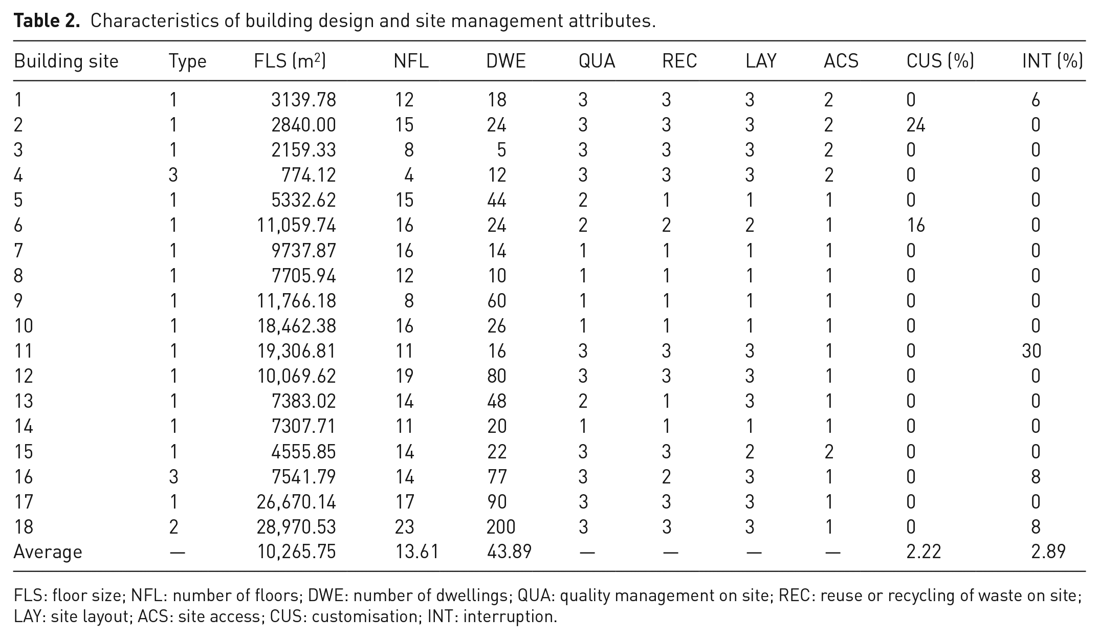
FLS: floor size; NFL: number of floors; DWE: number of dwellings; QUA: quality management on site; REC: reuse or recycling of waste on site; LAY: site layout; ACS: site access; CUS: customisation; INT: interruption.

The qualitative variables adopted a 3-level scheme (such as QUA and LAY), instead of dummy variables, to avoid an excess of parameters in the model. In a small sample, an excess number of parameters could provoke a statistical problem by reducing the degrees of freedom in the model.

The point in time in the construction stage when Waste is measured is an important element. The schedules of each project were collected and analysed. The method of planning in these buildings was the line of balance (LoB), which is regularly used in buildings with largely repetitive units (with several rather equal floors). The construction time of these projects ranged from 18 to 36 months. To equalise the construction times and allow for a better comparison, the schedules were standardised to a scale using a relative measure to Time, in a similar way to that used in the studies of Lu et al. (2016) and Villoria Sáez et al. (2014), describing the building evolution as a percentage of building deadlines:

Time: represents the time in the building schedule when a measure of waste was taken, in % of total schedule time.

For example, a measure collected in the ninth month of a schedule of 30 months was indicated as Time = 30%. The total waste was calculated as the sum of the partial waste measurements. Waste attributes are defined as:

Waste: Total waste, in m³;

Waste rate: The relationship between total waste and floor size, in m³ m^-2.

Waste rate was used to improve the comparability among the sampled buildings because there were significant differences in their size.

Not all buildings were accompanied through their entire schedule. The beginning and end of each on-site measurement were recorded. Both were listed as a percentage of progression in the building schedule. To increase comparability among the projects, a correcting factor was used, designed to compensate for partial measurement. Studies have proved the nonlinear nature of relationship between waste generation and the building schedule, but since the function of this relationship is not known, a linear extrapolation was adopted to simplify the procedure. This scheme is useful to allow making inferences in buildings with partial measurements. The total waste is calculated using equation (1):

W a s t e = W a s t e m e a s u r e d / (T i m e . E n d - T i m e . S t a r t)

(1)

where Waste is the estimation of total waste generated in a 100% period, in m³; Waste measured is the amount measured on site, in m³; Time.Start is the time in the building schedule when waste measurement started, in % of total schedule time; and Time.End is the time in the building schedule when waste measurement finished, in % of total schedule time.

Waste modelling using regression analysis

The main goal of regression analysis is to study the relationship between the waste generated and certain project attributes. Several configurations were tested in order to obtain explainable models, coherent with the behaviour observed at building sites. A general regression model follows equation (2) (Draper and Smith, 2014):

Y = a_{0} + a_{1} X_{1} + a_{2} X_{2} + \dots + a_{k} X_{k} + ε

(2)

where Y is the explained attribute; X₁, . . ., X_k are the explanatory attributes; a₀ is the intercept or constant of the equation; a₁, . . ., a_k are the coefficients, which are related to X₁, . . ., X_k; and ε is the error term.

The coefficients a_i were obtained using the ordinary least squares method. The model was verified following a conventional statistical analysis based on the coefficient of determination, p-values from a Student’s t-distribution, and Fisher–Snedecor F tests. Statistical tests evaluate the model and individual importance of included variables within a certain degree of accuracy, thus indicating the overall quality of the formulated model. A 5% error level was used in these models (Draper and Smith, 2014).

Results and discussion

The results obtained can be split in two parts. The first part of the results presents the waste measured at the building sites and the estimation of total waste. The second part presents models based on a regression analysis relating Waste and project attributes and examining the influence of building schedule on waste generation. Several functional forms and different compositions of the equation were explored using the variables presented in Table 2, maintaining the configuration in which all attributes reached the 5% level of significance (t) and analysis of variance (ANOVA) (F).

Waste measured on building sites

Waste was measured on a regular basis, recording 644 measurements for all buildings. Each measurement was associated with a specific time in the building schedule, following the relative scale adopted for Time. The values of waste measured each week were summed to calculate the total waste in each building. In the case of partial supervision of the building schedule, total waste was estimated using equation (1). The Waste rate was calculated based on Waste and FLS. Table 3 lists the data collected from the building sites.

Table 3.

Data measured and estimated: time period, waste measured, waste estimated, and waste rate.

Building site	Period of measurement		Waste measured(m³)	Waste(m³)^a	Waste rate(m³ m^-2)
Building site	Start time (%)	End time (%)	Waste measured(m³)	Waste(m³)^a	Waste rate(m³ m^-2)
1	0	60	441.78	736.30	0.235
2	0	100	643.28	643.28	0.227
3	10	84	272.50	368.24	0.171
4	0	100	98.30	98.30	0.127
5	4	44	336.00	840.00	0.158
6	50	100	682.50	1365.00	0.123
7	8	100	1271.50	1382.06	0.142
8	4	100	274.50	285.94	0.037
9	0	100	1832.66	1832.66	0.156
10	0	42	967.01	2302.40	0.125
11	42	100	2263.00	2694.05	0.140
12	22	74	1071.00	2059.61	0.205
13	28	78	676.00	1352.00	0.183
14	0	100	1251.00	1251.00	0.171
15	0	60	553.00	921.67	0.202
16	0	100	863.50	863.50	0.114
17	0	66	859.50	1302.27	0.049
18	0	48	2228.50	4642.71	0.160
Average	9.3	80.9	921.42	1385.61	0.151

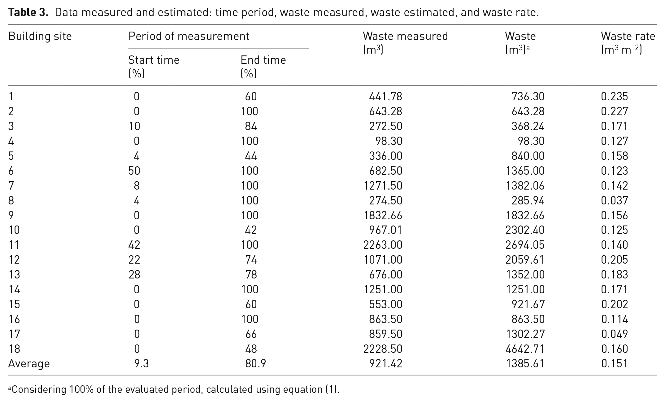
Considering 100% of the evaluated period, calculated using equation (1).

An initial analysis was based on a descriptive statistical analysis. The data collected were then represented in a graphical form, demonstrating the relationship of Waste and Waste rate with the quantitative design attributes; Figure 1 illustrates the plots of Waste calculated using equation (1) versus FLS and NFL (see Tables 2 and 3).

As observed from Figure 1, certain points deviated from the estimated values. The points can be removed to improve the models. However, they were not removed from consideration for two reasons. First, there was insufficient information to identify discrepant values and exclude cases. Second, the points did not belong to the same building or attribute. Regarding FLS (Figure 1, left), the largest deviations were those of buildings #17 and #18 (Table 2). Regarding NFL (Figure 1, right), the highest building had 23 floors (#18); however, the highest amounts of Waste were obtained from buildings #11 and #18 (Table 3). Therefore, all cases were preserved for the statistical analysis. The individual relationship was considered important, with R² = 0.7404 between Waste and FLS, and R² = 0.5109 between Waste and NFL.

The result of the isolated analysis provided insights for the ensuing multivariate modelling. There was evidence of a relationship, but at the same time there was a significant variation in both cases, which was not explained by a single attribute (only FLS or NFL, in this case). Therefore, this indicates that the explanation of changes in Waste needed a multivariate analysis.

Figure 2 shows the distribution of Waste rate and the same design attributes, to examine its isolated influence. An inverse relationship between Waste rate and FLS could be predicted, but with a small effect (expressed by R² = 0.1052). In other words, an increase in FLS seemed to slightly decrease the Waste rate values. Moreover, there was a weak relationship between the Waste rate and NFL (R² = 0.0011), suggesting an almost null consequence of NFL changes on Waste rate.

A more detailed analysis of the relationships presented in Figure 2 showed some peculiarities. There were buildings with similar values of FLS but different waste rates. For instance, cases with an FLS of nearly 8000 m² (buildings #8, #13, #14, and #16) had a Waste rate ranging from 0.037 to 0.183 m³ m^-2 (Figure 2, left, Tables 2 and 3). The maximum value was approximately five times greater than the minimum. In the same way, buildings with 11 or 12 floors (buildings #1, #8, #11, and #14) had a Waste rate ranging from 0.037 to 0.235 m³ m^-2. In this case, the difference between these values was approximately six times (Figure 2, right, Tables 2 and 3). Unlike Waste, Waste rate exhibited no clear relationship with FLS and NFL.

Developing models for Waste

The first model was designed to examine Waste in the stationary case (without Time). Based on data collected, the proposed model aimed to understand the relationship between the project characteristics and Waste. The fitted model is represented by equation (3). The results showed a satisfactory statistical relationship. The model had a calculated coefficient of R² = 0.8091, pointing toward an explanation of Waste variability of approximately 81%. The hypothesis of model validity was tested using ANOVA, which allows concluding on the meaning of regression models. In this case, the calculated value was F = 19.78, with a p = 2.65 × 10^-5, which met the conventional level of α = 5%. Tests on the explanatory variables used Student’s t-distribution. The value calculated for each attribute included in the model showed acceptance at the 5% level. The other variables in Table 2 were not included, as they did not meet the 5% level. The root-mean-square error (RMSE) was 454.74. Thus, the model satisfied the needs of a conventional statistical analysis and the hypothesis of a relationship, such as equation (3), could be admitted:

\begin{array}{l} W a s t e = 131.5941 + 0.05036 \times F L S \\ + 0.1890 \times N F L^{3} + 42.8287 \times I N T \end{array}

(3)

The model presented in equation (3) suggested the influence of three attributes on the total Waste. The influence of FLS was positive when the other attributes were constant, and the calculated coefficient implied 50.4 m³ of waste was generated for every 1000 m² of built-up area. The second influencing attribute was NFL. The influence of this attribute on the equation was nonlinear; therefore, the volume of Waste changed depending on the number of levels. One level more than the average number of floors increased the Waste by approximately 112.9 m³. Interruptions (INT) in the construction added 42.8 m³ of waste for each 1% of interruption in a normal schedule (for instance, 1% stands for 1 week in a 24-month schedule).

Developing models for Waste with Time

The second regression model explored the influence of building stages, including the variable Time, and used 644 measurements of waste in the 18 buildings investigated. The results obtained indicated a satisfactory statistical relationship. The coefficient of determination (R² = 0.9141) showed a 91% level of understanding of Waste variability with the set of explanatory attributes. The model’s ANOVA estimate reached F = 2273.40, with a p-value near zero. Through t-tests, the combinations of Time were approved at the 5% level. The RMSE calculated was 0.168. As the model presented in equation (4) respects statistical assumptions, it may be acceptable to use. Equation (4) includes three configurations of Time:

\begin{array}{l} W a s t e (%) = 0.01401 \times T i m e - 1.0173 \times 10^{- 4} \\ \times T i m e^{2} + 6.1531 \times 10^{- 7} \times T i m e^{3} \end{array}

(4)

This model was based on the estimation of Waste at each stage of the building schedule. It is represented as Waste(%), indicating that the calculated values were linked to a time in the building schedule. Essentially, measures obtained at building sites characterise partial waste measures. Time represents a relative scale of construction measured after the time forecasted in the building schedule, and it was included in the model in a nonlinear format (including squared and cubic terms of time). Other models were tested, including a model with Time components in fourth and fifth degrees, with no significant advantage. Nevertheless, they reached similar results, also presenting a slight S shape. The project attributes (Table 2) were also tested, with no significant influence on equation (4). A nonlinear relationship between the percentages of Waste and Time (Figure 3) was thus perceived.

The contributions of the different construction stages, calculated by equation (4), showed a slight S shape. The portion of waste generated was similar in the first and third stages of the building schedule. The first 33% of the schedule was associated with 37.4% of the total waste generated. The 34%–66% period was responsible for 28.5%, and the last part of the building phase (67%–100%) corresponded to 34.1% of waste generated at the building site.

Discussion

Several insights into the results are presented in this section. The method used to collect waste generation data on-site worked satisfactorily. The team at work, including the production and administrative staff, accepted and assimilated the waste management plan, contributing to the development of the study. The waste measured in partial schedules was converted to the estimated Waste and allowed performing an analysis of the total waste generated at building sites. The first estimate of the average Waste rate was 0.151 m³ m^-2. This figure was comparable with the values found in other studies (Table 1).

Two models were produced using the data collected, based on a regression analysis. A general overview of the statistical behaviour of the proposed models is presented in Table 4.

Table 4.

Statistical results on the models.

Model (equation)	RMSE	R²	Attributes
Waste (equation (3))	454.74	0.8091	FLS, NFL, INT
Waste and Time (equation (4))	0.1683	0.9141	Time

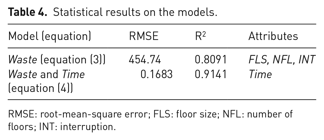
RMSE: root-mean-square error; FLS: floor size; NFL: number of floors; INT: interruption.

Analysing equation (3), it indicated that Waste increases with the increase in FLS, NFL, and INT. While FLS and NFL are present in other studies on waste generation (such as Kern et al., 2015; Villoria Sáez et al., 2015), the latter is an important and relatively unknown contributor. It is related to building safety violations, such as incorrect scaffolding, detected by labour inspectors, and it interrupts the work for some time. In addition to an increase in cost and construction delays, the amount of waste increases because new material is used to substitute the building safety structures with new ones, making the old structures obsolete. Certain attributes related to site organisation, such as QUA, ACS, LAY, and REC are not evaluated in this model. It could be expected that a greater control and general organisation on the building site would reduce waste, but the influence of these attributes was less than the minimum level of 5%. The model produced to explain total waste (equation (3)) has three attributes; thus, it is evident that waste generation is based on a set of attributes. This model could help expand waste management plans when used in comparison with the simple estimated average of waste rate.

Equation (4) analyses the effect of time on waste generation. The regression shows a nonlinear effect, with quadratic and cubic terms of Time, increasing waste with increasing time, but with certain changes in each third of the building schedule. The variation in waste generation with time is represented through an S-shaped curve (Figure 3). The shape of the curve can be related to the schedule formats of the evaluated buildings. In projects planned to use the LoB method, S-shaped curves of costs and resource consumption are generally obtained (Halpin and Woodhead, 1976). Therefore, it is not surprising that waste generation also follows this shape.

Comparing these results with studies found in the literature (Akinade et al., 2018; Kern et al., 2015; Lee et al., 2016; Villoria Sáez et al., 2014, 2015; Wu et al., 2015), several similarities can be observed in the models, in terms of the model format and attributes included. The coefficient of determination in these studies ranges from 0.694 to 0.998, which is comparable with the results presented in Table 4. The studies by Lu et al. (2016) and Villoria Sáez et al. (2014) indicate nonlinear models with S-shaped curves representing the relationship between time and waste.

This study obtained results that confirm those in the literature. It is remarkable to reach similar results in a different country and construction context. However, there are some limitations to this study. The measurements taken on site contained mixed waste. Thus, it is difficult, or maybe impossible, to analyse the main type of waste generated at each stage of construction. This information could improve waste plans, indicating the level of focus on details. Another issue is that some of these projects are built following a sales-based scheme. In this case, construction depends partially on sales, and the construction speed could change after economic resources become available.

Conclusions

Construction waste corresponds to a significant portion of the total waste produced by the society. Solutions that reduce construction waste generation are a challenge in the construction industry. This study contributes to the understanding of waste generation at construction sites through statistical modelling.

A method for waste measurement was developed, and data were obtained from selected building sites. The proposed regression models had a satisfactory statistical performance and thus may be acceptable for estimating generated wastes to guide management plans. The models propose a comprehensive relationship between waste and building characteristics. The model to estimate total Waste had a simple yet effective linear format and was based on building characteristics, data for which may be collected directly from the project sites. The second model considered Time, and it indicated a link between waste generation and building schedules. This model suggested a small nonlinear influence of the Time attributes on Waste, through an S-shaped curve.

In summary, the models based on regression analysis could contribute to waste generation understanding by showing the most relevant attributes and their weights. Under these circumstances, they can be used to predict waste generation in projects with similar characteristics. The models can preview waste before construction commences and help builders improve on-site waste management. Therefore, this approach could be used to reduce cost and waste in new projects.

Footnotes

Acknowledgements

The authors wish to acknowledge also the support of Brazilian agencies Fundação de Amparo à Pesquisa do Estado do Rio Grande do Sul (FAPERGS) and Conselho Nacional de Pesquisa (CNPq).

Declaration of conflicting interests

The authors declared no potential conflicts of interest with respect to the research, authorship, and/or publication of this article.

Funding

The authors disclosed receipt of the following financial support for the research, authorship, and/or publication of this article: This study was financed in part by the Coordenação de Aperfeiçoamento de Pessoal de Nível Superior – Brazil (CAPES) – Finance Code 001.

ORCID iD

Marco Aurélio Stumpf González

References

Ajayi

Oyedele

Bilal

, et al. (2017) Critical management practices influencing on-site waste minimization in construction projects. Waste Management 59: 330–339.

Akinade

Oyedele

Ajayi

, et al. (2018) Designing out construction waste using BIM technology: Stakeholders’ expectations for industry deployment. Journal of Cleaner Production 180: 375–385.

Alfaia

RGSM

Costa

Campos

(2017) Municipal solid waste in Brazil: A review. Waste Management and Research 35: 1195–1209.

Bakchan

Faust

(2019) Construction waste generation estimates of institutional building projects: Leveraging waste hauling tickets. Waste Management 87: 301–312.

Bakshan

Srour

Chehab

, et al. (2015) A field based methodology for estimating waste generation rates at various stages of construction projects. Resources, Conservation and Recycling 100: 70–80.

Bakshan

Srour

Chehab

, et al. (2017) Behavioral determinants towards enhancing construction waste management: A Bayesian network analysis. Resourses, Conservation and Recycling 117: 274–284.

Bossink

BAG

Brouwers

HJH

(1996) Construction waste: Quantification and source evaluation. Journal of Construction Engineering and Management 122: 55–60.

Brönstrup

(2010) Diretrizes para implantação de um sistema de gerenciamento de resíduos de construção e demolição para o município de Gramado-RS. Master’s thesis, PPGEC, UNISINOS, São Leopoldo, Brazil (in Portuguese). Available at: http://repositorio.jesuita.org.br/handle/UNISINOS/4636 (accessed 1 July 2019).

Chen

(2017) Identifying factors influencing demolition waste generation in Hong Kong. Journal of Cleaner Production 141: 799–811.

10.

Cooke

Williams

(2014) Construction Planning, Programming and Control. 3rd edn. Oxford, UK: Wiley Blackwell.

11.

Draper

Smith

(2014) Applied Regression Analysis. New York: John Wiley & Sons.

12.

Formoso

Soibelman

Cesare

C de

, et al. (2002) Material waste in building industry: Main causes and prevention. Journal of Construction Engineering and Management 128: 316–325.

13.

Gangolells

Casals

Forcada

, et al. (2014) Analysis of the implementation of effective waste management practices in construction projects and sites. Resources, Conservation and Recycling 93: 99–111.

14.

Guerra

Bakchan

Leite

, et al. (2019) BIM-based automated construction waste estimation algorithms: The case of concrete and drywall waste streams. Waste Management 87: 825–832.

15.

Halpin

Woodhead

(1976) Design of Construction and Process Operations. New York: John Wiley & Sons.

16.

Hao

Hill

Shen

(2008) Managing construction waste on-site through system dynamics modelling: The case of Hong Kong. Engineering, Construction and Architectural Management 15: 103–113.

17.

Islam

Nazifa

Yuniarto

, et al. (2019) An empirical study of construction and demolition waste generation and implication of recycling. Waste Management 95: 10–21.

18.

ITeC (2012) Banco estructurado de datos de elementos constructivos (BEDEC). Barcelona: Instituto de Tecnologia de la Construcción de Cataluña (ITeC) – Dirección general de Medioambiente (in Spanish). Available at: http://itec.es/informacio/PreciosConstruccion.aspx (accessed 1 July 2019).

19.

Jain

Singhal

Jain

(2018) Construction and demolition waste (C&DW) in India: Generation rate and implications of C&DW recycling. International Journal of Construction Management. Epub ahead of print 18 October 2018. DOI: 10.1080/15623599.2018.1523300.

20.

Katz

Baum

(2011) A novel methodology to estimate the evolution of construction waste in construction sites. Journal of Waste Management 31: 353–358.

21.

Kern

Dias

Kulakowski

, et al. (2015) Waste generated in high-rise buildings construction: A quantification model based on statistical multiple regression. Waste Management 39: 35–44.

22.

Kim

Hong

Park

, et al. (2017) An estimation framework for building information modeling (BIM)-based demolition waste by type. Waste Management and Research 35: 1285–1295.

23.

Kupusamy

Nagapan

Abdullah

, et al. (2019) Construction waste estimation analysis in residential projects of Malaysia. Engineering, Technology and Applied Science Research 9: 4842–4845.

24.

Lafayette

KPV

Paz

DHF

Holanda

MJO

, et al. (2018) Analysis of generation and characterization of construction and demolition waste on construction sites in the city of Recife, Brazil. Matéria (Rio Janeiro) 23: 1–16.

25.

Lee

Kim Seungho Kim Sangyong (2016) Development of hybrid model for estimating construction waste for multifamily residential buildings using artificial neural networks and ant colony optimization. Sustainability 8: 870. DOI: 10.3390/su8090870.

26.

Ding

, et al. (2013) A model for estimating construction waste generation index for building project in China. Resources, Conservation and Recycling 74: 20–26.

27.

Zhang

Ding

, et al. (2016) Developing a quantitative construction waste estimation model for building construction projects. Resources, Conservation and Recycling 106: 9–20.

28.

Liu

Chen

Tang

(2018) A method for estimation of the on-site construction waste quantity of residential projects. In: Yaowu

Yimin

Geoffrey

, et al. (eds) International Conference on Construction and Real Estate Management – ICCREM 2018, 125–131. ASCE, Charleston, SC: Modernization of Management Committee of the China Construction Industry Association/Construction Institute of ASCE.

29.

Peng

Chen

, et al. (2016) The S-curve for forecasting waste generation in construction projects. Waste Management 56: 23–34.

30.

Magalhães

de, Danilevicz

ADMF

Saurin

(2016) Reducing construction waste: A study of urban infrastructure projects. Waste Management 67: 265–277.

31.

Mália

Brito

J de

Bravo

(2011) Indicadores de resíduos de construção e demolição para construçoes residenciais novas. Ambiente Construído 113: 117–130 (in Portuguese).

32.

Marques

(2007) Resíduos da Construção Civil em Araguari-MG: Do Diagnóstico à Proposta de um Modelo Gerencial Proativo. Master’s Thesis, Universidade Federal de Uberlândia, Uberlândia, Brasil (in Portuguese). Available at: https://repositorio.ufu.br/handle/123456789/14243 (accessed 1 July 2019).

33.

McDonald

Smithers

(1998) Implementing a waste management plan during the construction phase of a project: A case study. Construction Management and Economics 16: 71–78.

34.

Medina Jimenez

Bereche

Nebra

(2019) Three municipal solid waste gasification technologies analysis for electrical energy generation in Brazil. Waste Management and Research 37: 631–642.

35.

Menegaki

Damigos

(2018) A review on current situation and challenges of construction and demolition waste management. Current Opinion in Green and Sustainable Chemistry 13: 8–15.

36.

Mercader Moyano

Ramírez de Arellano-Agudo

Cózar-Cózar

, et al. (2017) Sistema BIM de cuantificación automática de los residuos de construcción y demolición. Estudios del Hábitat 15: 24 (in Spanish).

37.

Oliveira

(2008) Desenvolvimento de ferramenta para apoio à gestão de resíduos de construção e demolição com uso de geoprocessamento: caso Bauru-SP. Master’s Thesis, Centro de Ciências Exatas e de Tecnologia, Universidade Federal de São Carlos, São Carlos, Brasil (in Portuguese). Available at: https://repositorio.ufscar.br/handle/ufscar/4240 (accessed 1 July 2019).

38.

Paz

DHF

Lafayette

KPV

Sobral

(2018) GIS-based planning system for managing the flow of construction and demolition waste in Brazil. Waste Management & Research 36: 541–549.

39.

Penteado

CSG

Rosado

(2016) Comparison of scenarios for the integrated management of construction and demolition waste by life cycle assessment: A case study in Brazil. Waste Management and Research 34: 1026–1035.

40.

Pinto

(1999) Metodologia para a gestão diferenciada de resíduos sólidos da construção urbana. PhD Thesis, Escola Politécnica, Universidade de São Paulo, São Paulo (in Portuguese). Available at: http://www.academia.edu/download/46261238/Metodologia_para_gestao_diferenciada_de_RCD_-_Pinto.pdf (accessed 1 July 2019).

41.

Poon

Ann

(2001) On-site sorting of construction and demolition waste in Hong Kong. Resources, Conservation and Recycling 32: 157–172.

42.

Ram

Kalidindi

(2017) Estimation of construction and demolition waste using waste generation rates in Chennai, India. Waste Management & Research 35: 610–617.

43.

Roaf

Fuentes

Thomas

(2012) Ecohouse: A Design Guide. 4th edn. Oxford: Architectural Press/Elsevier.

44.

Sardá

(2003) Diagnóstico do resíduo da construção civil gerado no município de BlumenauSC: Potencialidades de uso em obras públicas. Master’s Thesis, Universidade Federal de Santa Catarina, Florianópolis, Brasil (in Portuguese). Available at: https://repositorio.ufsc.br/handle/123456789/85474 (accessed 1 July 2019).

45.

Skoyles

(1987) Waste Prevention on Site. London: Mitchell.

46.

Soibelman

(1993) As perdas de materiais na construção de edificações: sua incidência e seu controle. Master’s Thesis, Universidade Federal do Rio Grande do Sul, Porto Alegre, Brasil (in Portuguese). Available at: http://www.lume.ufrgs.br/handle/10183/1701 (accessed 1 July 2019).

47.

Solís-Guzmán

Marrero

Montes-Delgado

, et al. (2009) A Spanish model for quantification and management of construction waste. Waste Management 29: 2542–2548.

48.

Song

Wang

Liu

, et al. (2017) Development of a hybrid model to predict construction and demolition waste: China as a case study. Waste Management 59: 350–361.

49.

Souza

UEL

de, Paliari

Agopyan

, et al. (2004) Diagnóstico e combate à geração de resíduos na produção de obras de construção de edifícios: uma abordagem progressiva. Ambiente Construído 4: 33–46.

50.

Villoria Sáez

Astorqui

JSC

del Río Merino

, et al. (2018) Estimation of construction and demolition waste in building energy efficiency retro fitting works of the vertical envelope. Journal of Cleaner Production 172: 2978–2985.

51.

Villoria Sáez

Osmani

(2019) A diagnosis of construction and demolition waste generation and recovery practice in the European Union. Journal of Cleaner Production 241: 118400.

52.

Villoria Sáez

Porras-Amores

del Río Merino

(2015) New quantification proposal for construction waste generation in new residential constructions. Journal of Cleaner Production 102: 58–65.

53.

Villoria Sáez

del Río Merino

Porras-Amores

, et al. (2014) Assessing the accumulation of construction waste generation during residential building construction works. Resources, Conservation and Recycling 93: 67–74.

54.

Villoria Sáez

del Río Merino

Porras-Amores

(2012) Estimation of construction and demolition waste volume generation in new residential buildings in Spain. Waste Management & Research 30: 137–146.

55.

Vilventhan

Ram

Sugumaran

(2019) Value stream mapping for identification and assessment of material waste in construction: A case study. Waste Management and Research 37: 815–825.

56.

Duan

Zheng

, et al. (2016) Demolition waste generation and recycling potentials in a rapidly developing flagship megacity of South China: Prospective scenarios and implications. Construction and Building Materials 113: 1007–1016.

57.

Ann

Shen

, et al. (2014) Quantifying construction and demolition waste: An analytical review. Waste Management 34: 1683–1692.

58.

Fan

Liu

(2015) Forecasting construction and demolition waste using gene expression programming. Journal of Computing in Civil Engineering 29: 04014059.

59.

Yang

Xia

Thompson

, et al. (2017) Urban construction and demolition waste and landfill failure in Shenzhen, China. Waste Management 63: 393–396.

60.

Zhang

Zheng

Duan

, et al. (2019) Differences of methods to quantify construction and demolition waste for less-developed but fast-growing countries: China as a case study. Environonment Science and Pollution Research 26: 25513–25525.