
Abstract
This article presents a theoretical work on liquid heat-up in the case of a pool fire. It is assumed that the convective currents occurring within the upper layer of the liquid are induced by Rayleigh–Bénard instabilities that are caused by in-depth radiation. The upper layer depth has been estimated based on the analytical solution of a one-dimensional Fourier’s equation for the temperature with a source term for in-depth radiation. The model has been assessed against experimental data for a 9-cm-diameter methanol steady-state pool fire and three different liquid depths (18, 12 and 6 mm). The general trend, that is, increase in the upper layer depth as the bottom boundary temperature increases, is well captured. In order to ensure that the well-mixed upper layer is at a temperature near the boiling point (as suggested by the experimental data), an improvement is proposed based on a radiative heat balance integral method. In addition to the above, a novel methodology is developed for the calculation of the ‘effective’ thermal conductivity as a means to circumvent detailed calculations of heat transfer within the liquid.
Introduction
Quite extensive research is carried out on the numerical modelling of liquid pool fires, given the potential hazard induced by these types of fires. More specifically, computational fluid dynamics (CFD) is an advanced technique that is extensively being used for the simulation of pool fires. However, the current developments and applications are mostly devoted to gas phase aspects, for example, combustion and thermal radiation modelling. 1 In this case, the burning (evaporation) rate is prescribed according to an experimentally measured value or an estimate based on a semi-empirical correlation. In reality, the burning rate is strongly coupled to the heat feedback from the flame (and, eventually, other ‘external sources’ such as the smoke layer, ceiling and walls in an enclosure fire). The higher the heat feedback, the higher the burning rate (because of a more intense liquid heat-up and evaporation) and vice versa. Therefore, in order to perform fully predictive simulations of liquid pool fires, the coupling liquid phase–gas phase must be considered. The most advanced approach would be to solve the full set of Navier–Stokes equations for the liquid phase (as it is the case for the gas phase), as recently attempted in Fukumoto et al. 2 However, a more thorough and extensive assessment of this approach is still required. Furthermore, such approach is believed to require prohibitive amounts of computational resources for ‘practical’ fire dynamics simulations, considering the resources that would have been already allocated for the gas phase. A significantly simpler approach consists of solely solving the heat-up of the liquid layer and not the momentum equation therein, using a one-dimensional (1D) Fourier’s equation, as if it was a thermally thick solid. By doing so, the convective currents in liquid fuels during pool burning, as pointed out in Fukumoto et al. 2 and Sikanen and Hostikka, 3 are neglected. The idea is then to model ‘indirectly’ the convective currents, keeping the 1D Fourier’s equation as a general framework. This has been mainly developed in Sikanen and Hostikka 3 where the main assumption is that ‘in large pool fires, the main source of convective motions is buoyancy-generated by in-depth radiation absorption’. Therefore, the work presented in Sikanen and Hostikka 3 is mainly centred around two aspects: (1) the modelling of a radiative source term in the heat conduction equation, including the estimation of the absorption coefficients of liquids and (2) the modelling of an ‘effective thermal conductivity’, which has been referred to above as an ‘indirect’ modelling of convective currents that enhance heat transfer within the liquid. As opposed to Sikanen and Hostikka, 3 the purpose of this work is not to implement the proposed sub-models in CFD simulations and assess the latter against transient profiles and steady-state values of the burning rate for a wide range of liquids and pan diameters. The intent is rather to take a step back and focus specifically on the thermal structure of the liquid and the modelling of an ‘effective’ thermal conductivity coefficient. The assessment of the proposed work is based on the experimental profiles of liquid temperature provided in Vali et al. 4 bearing in mind that some of the profiles discussed in Sikanen and Hostikka 3 were ‘clearly unphysical’.
Experimental data
To the best of the author’s knowledge, the most comprehensive experimental work on heat transfer within the liquid in a pool fire is described in Vali et al. 4 for a 9-cm-diameter methanol steady-state pool fire and three different liquid depths (18, 12 and 6 mm), maintaining the bottom boundary temperature at several values between −10°C and 50°C. More specifically, the velocity field within the liquid fuel was determined by particle image velocimetry (PIV) and the temperature was measured by type K thermocouple probes. A distinct two-layer thermal structure was depicted and estimates of the thickness of the lower layer are provided in Vali et al. 4 Given the fact that in Vali et al. 4 a steady fuel level was maintained in the pool, the thickness of the top layer can be easily retrieved from the data displayed therein. The uniform temperature within the vaporizing layer was attributed to two-counter rotating vortices. The first vortex, close to the pool wall, is explained by the ‘buoyancy force near the pool wall and shear stress forces at the liquid–gas interface’. Several potential reasons are provided for the development of the second vortex, for example, ‘the liquid–gas interface shear force’ or the ‘non-uniformity of local evaporation rate at the pool surface’. In Inamura et al., 5 it is stated that in-depth (radiation) absorption leads to ‘in-depth temperatures’ higher than the surface temperature, generating thus a convective current (due to Rayleigh convection) that drives the mixing within the boiling layer. This phenomenon causes the temperature profile across the vaporizing fuel layer to be uniform. Rayleigh convection has been confirmed experimentally in Inamura et al., 5 using holographic interferometry for a toluene pool fire. Generally speaking, the two-layer thermal structure described in Vali et al. 4 is suitable for ‘thin’ pools. A more ‘complete’ description of the liquid thermal structure is provided in Hayasaka 6 where, for sufficiently ‘deep pools’, beneath the ‘preheating layer’, there is a ‘bottom fuel layer’ where the fuel temperature does not vary substantially (see Figure 1).
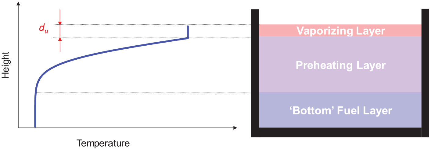
Thermal structure within the liquid in the case of a pool fire.
Based on the thermal structure displayed in Figure 1, for ‘thin’ pools (as in Vali et al. 4 ), the upper layer is the vaporizing layer and the lower layer is the preheating layer.
Numerical modelling
The numerical simulation of in-depth radiation has been undertaken in Inamura et al. 5 and Garo et al. 7 by considering a source term in the governing energy equation (for the liquid) where the radiative flux at a given depth within the liquid is derived by applying the ‘classical attenuation law’, that is, Beer–Lambert law, to the radiative heat flux at the fuel surface using a mean (spectrally averaged) absorption coefficient. As explained in Garo et al., 7 this approach generally leads to a ‘temperature inversion layer’ that is not observed experimentally. This is explained in Garo et al. 7 by the fact that ‘the onset of convective currents (Rayleigh effect) generated by the radiation absorption near the surface [is] not considered in the theoretical model’. This has been one of the main modelling aspects addressed in Sikanen and Hostikka 3 and which will be recalled in the following sub-section in order to put this work into context and better highlight the novelties with respect to the developments proposed in Sikanen and Hostikka. 3
Approach of Sikanen and Hostikka
In Sikanen and Hostikka, 3 ‘the 1D heat conduction equation for liquid temperature is applied in the x-direction pointing into the liquid (the point x = 0 represents the surface)’ and it reads

where ρ, k, c and T are the density, the thermal conductivity, the specific heat and the temperature of the liquid, respectively. The variables t and

where
The key parameters of interest here are k,
The volumetric radiative heat source term in the heat conduction equation is calculated in Sikanen and Hostikka 3 by solving the transport of heat radiation inside the liquid layer using a ‘two-flux’ model based on the Schuster–Schwarzschild approximation.
In-depth radiation creates a ‘volumetric heat source evenly distributed over the liquid layer thickness’ (see Figure 2) and which can be expressed as 3

where L is the liquid layer thickness.
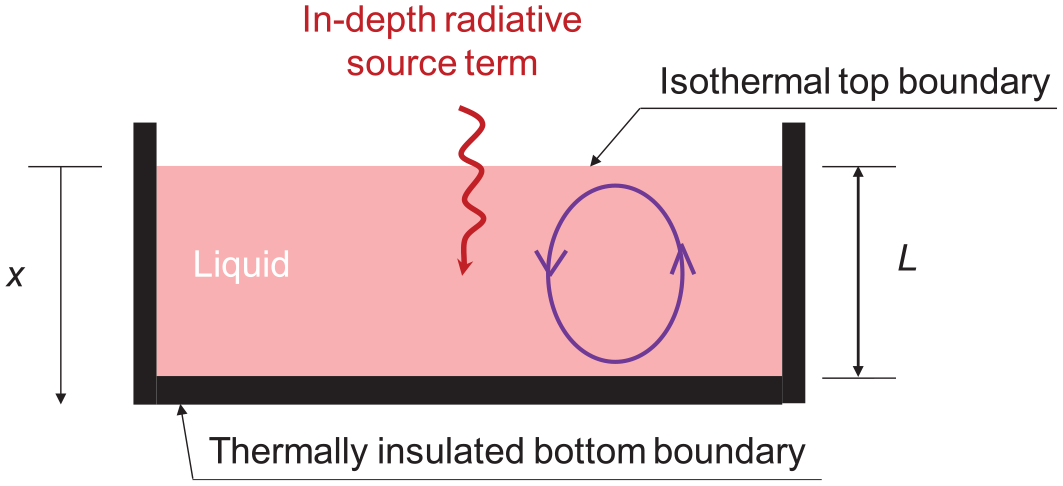
A schematic of in-depth radiation treatment in pool fires in Sikanen and Hostikka. 3
Such volumetric heat source will generate convective currents which will increase heat transfer within the liquid. This increase in heat transfer is ‘indirectly’ modelled by increasing the actual thermal conductivity of the liquid, k, to the so-called ‘effective thermal conductivity’, keff, according to the following equation

where Nu i is the Nusselt number. It is important to mention at this level that we refer here to an ‘internal’ Nusselt number (within the liquid) and not the Nusselt number used for convective heat transfer at the interface between the liquid and the surrounding gas. In Sikanen and Hostikka, 3 Nu i is calculated from a correlation for internally heated horizontal plane layer (recall here the volumetric heat source in equation (1)) with isothermal top boundary and thermally insulated bottom boundary

The variable Ra i denotes the internal Rayleigh number calculated in Sikanen and Hostikka 3 as

where g is the gravitational acceleration and β, ν and α are the coefficient of thermal expansion, the kinematic viscosity and the thermal diffusivity of the liquid, respectively. The variable

and the variable η is a normalized length scale associated with the source distribution and calculated as

where κ is the effective absorption coefficient of the liquid. The latter parameter is calculated using an elaborate algorithm described in detail in Sikanen and Hostikka. 3
A significant source of uncertainty in the above methodology (and pointed out in Sikanen and Hostikka 3 ) is that the effective thermal conductivity is calculated using the full depth, L, of the liquid as a characteristic length scale (see equation (6)). While this approach may be suitable for a ‘relatively thin layer of fuel’, it might not be appropriate for deep pools where the convective currents would be localized in the thin top layer of the liquid.
In the next section, we propose a novel treatment of in-depth radiation in liquid pool fires.
Novel approach
Definition of the Rayleigh and Nusselt numbers
The main idea developed in this work (and originally proposed in Beji and Merci 8 ) is to use, instead of equation (6), the ‘classical’ definition of the Rayleigh number

where T1 and T2 are the bottom and surface temperatures of the fluid layer, respectively, and
The effective thermal conductivity in the liquid pool can be calculated using equation (4) considering the case of a ‘horizontal cavity heated from below’ for which the Nusselt number is calculated, instead of equation (5), as 9

where Pr is the liquid Prandtl number.
As described in Beji and Merci, 8 the use of equation (10) is justified by the fact that in-depth radiation heats up the liquid beneath the surface, leading to the top portion of the liquid (subjected to in-depth radiation) to be hotter at its bottom (i.e. heating from below). This is somewhat counter-intuitive, given that the flame is heating the liquid from the top. More details will be provided hereafter.
In the remainder of the article, the objective is to develop and explain two methods for the calculation of (1) the length scale and (2) the temperature difference that are used to estimate Ra i and, consequently, Nu i and keff.
Analytical solution of the temperature profile
In the proposed approach, we seek to find an analytical solution for heat conduction within the liquid, including in-depth radiation in order to derive an explicit expression for the characteristic length scale that is needed for the calculation of Ra i and thus, Nu i and keff.
The 1D equation for heat conduction at steady state and including in-depth radiation reads 7

where
Based on the classical attenuation law, that is, Beer’s law, the radiative flux is expressed as 7

where
Inserting equation (12) into equation (11) gives

When using the BCs

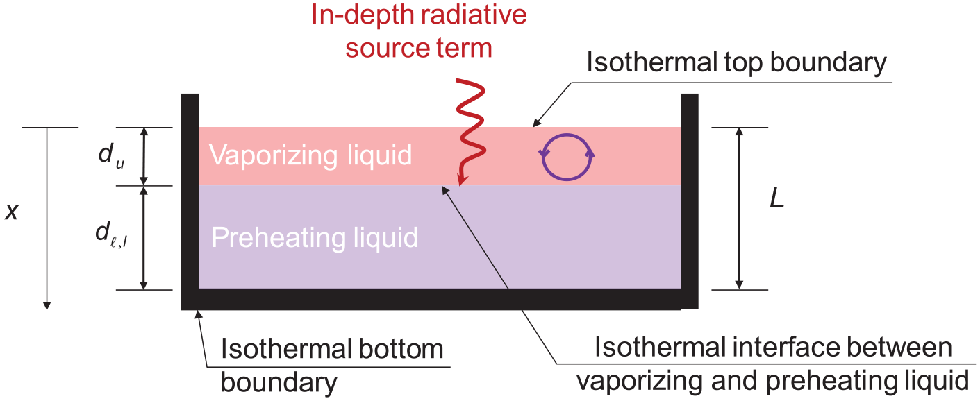
A schematic of in-depth radiation treatment in pool fires in this work.
An illustration of the obtained liquid temperature profile for one of the cases examined experimentally in Vali et al. 4 is displayed in Figure 4. As expected, the peak temperature does not occur at the surface but at a specific depth form the surface, yielding a so-called ‘inverse temperature profile’ under the effect of in-depth radiation.
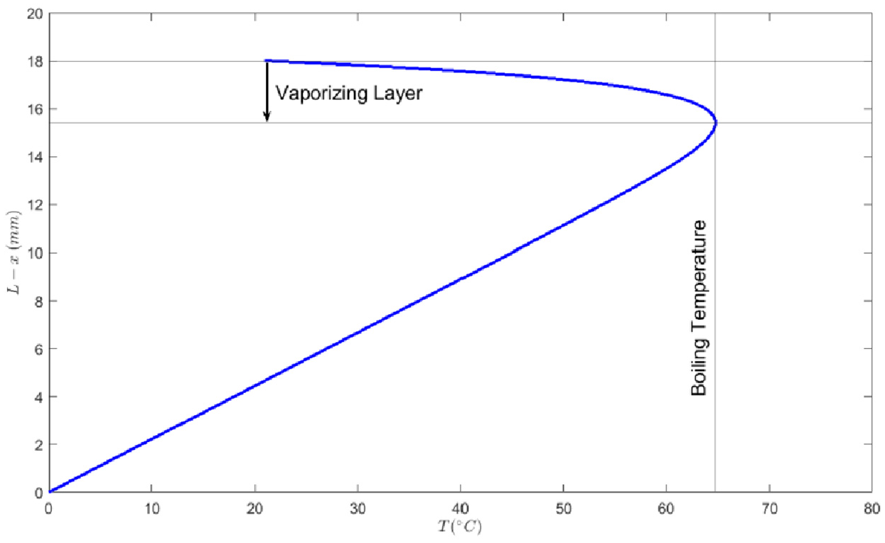
Liquid temperature profile for a case examined in Vali et al.
4
with the following parameters: Ts = 21°C, Tb = 0°C, κ = 1000 m−1,
Method 1 based on the locus of the peak temperature
Assuming that the well-mixed layer spans across the liquid layer from the surface up to the location of the peak temperature within the liquid, the analytical expression of
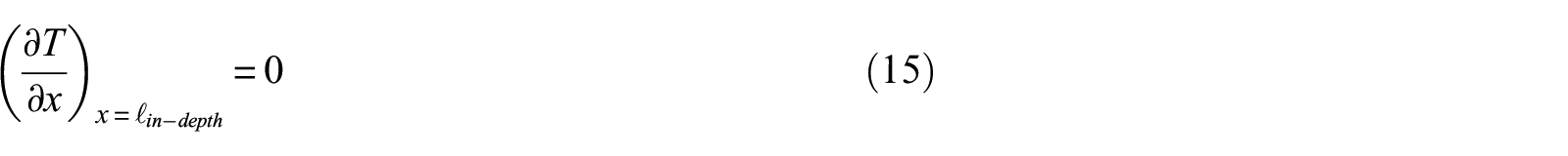
Applying equation (15) for the temperature profile obtained in equation (14) gives
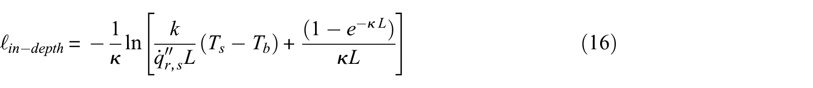
Note that at depths below
The main aspects that have been developed so far can be visualized in Figure 3, which gives an overall view of the thermal structure within the liquid and in which
From a mathematical standpoint, it is important to note that equation (16) gives a solution to the problem only if the following condition is satisfied

where ΔT = Ts – Tb. This is because the sum of the terms between brackets in equation (16) (and which is strictly higher than zero) should be strictly lower than 1 so that the natural logarithm gives a negative number and, consequently,
Let us examine now expression (17) from a physical standpoint. If, for given constant values of
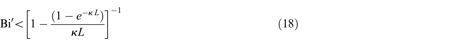
where

is a (so-called here) ‘modified’ Biot number which, as opposed to the ‘classical’ Biot number, does not compare the relative importance of convective to radiative heat transfer in terms of resistances, that is,
We note also that the condition
Before moving to the assessment of the developed method against experimental data, it is very important to bear in mind two important aspects related to the methodology described above
As opposed to Beji and Merci,
8
the top surface temperature is not assumed to be the boiling temperature of methanol (i.e. Ts = Tboiling = 64.8°C),
3
but it is calculated in such a way that the peak temperature at
Based on the above, the surface temperature becomes an unknown of the problem. In fact, Ts should not be regarded as a ‘true’ top BC. The latter is imposed by setting a constant radiative heat flux. This is because the main objective in this work is to calculate Ra
i
(see equation (9)) in order to able to calculate the Nu
i
and thus the effective conductivity. This is done if one is able to estimate the length scale for in-depth radiation and the temperature difference (in the method described above that would be Tboiling – Ts). To sum up, the inputs are
Equation (16) (with
Properties of methanol.
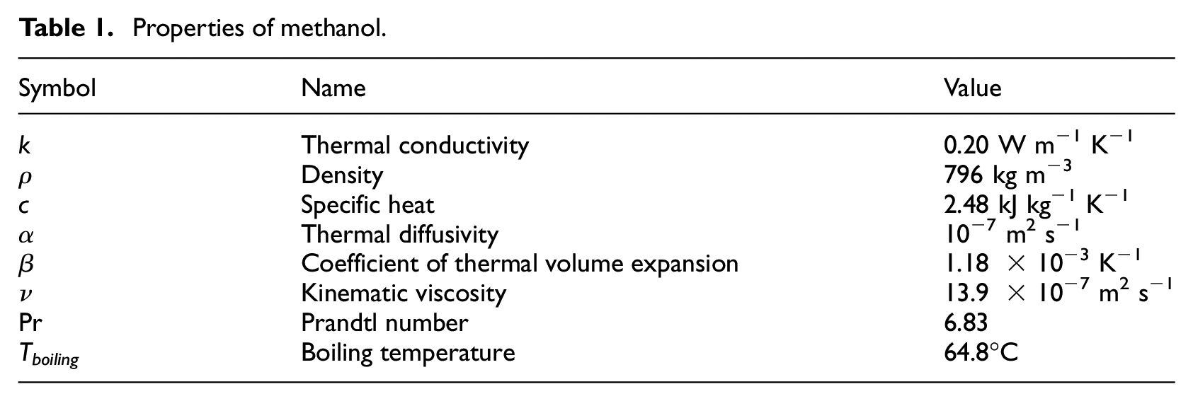
The results displayed in Figure 5 (left sub-figures) for the non-dimensional upper layer depth, that is, du/L, show that the ‘nearly’ constant upper layer depth of about du = 0.28 ± 0.03 L for L = 18 mm is best captured with κ = 500 m−1. When the bottom temperature Tb is between 35°C and 50°C, a value of κ = 1000 m−1 gives also a good agreement with the experimental data. In fact, the experimental data for L = 18 mm is well bounded by the calculations with κ between 500 and 1000 m−1 (see Figure 5(a)). For L = 12 mm (see Figure 5(c)), a more ‘suitable’ range for κ spans from 300 to 500 m−1. The experimental trend for L = 6 mm has been more difficult to capture (see Figure 5(e)) in that a value of κ = 500 m−1 appears to be ‘suitable’ for a bottom temperature Tb above 30°C. For Tb < 30°C, higher values of κ (up to 2000 m−1) give a better agreement. Nevertheless, the fact that there is no well-mixed upper layer (i.e. du = 0 mm) at Tb = 4°C could not be captured. One explanation could be that surface tension–driven convection, which becomes important in thin pools, is not considered in the current modelling.
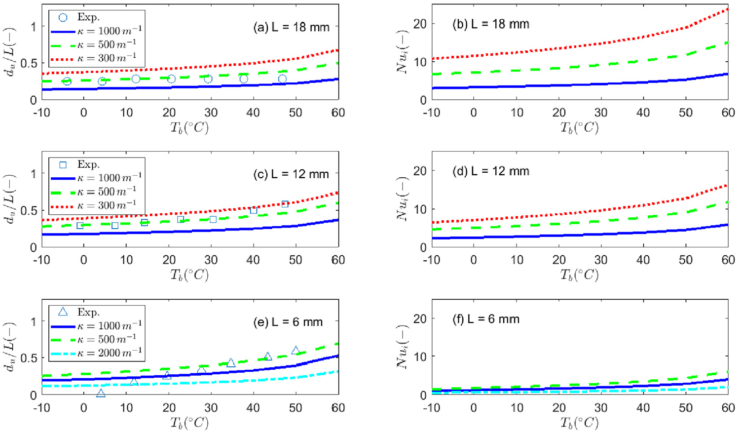
Results with method 1 for a 90-mm-diameter methanol pool fire as a function of the bottom layer temperature. A comparison between the experimental measurements 4 and numerical predictions of the non-dimensional upper layer depth (left) and predicted Nu i (right).
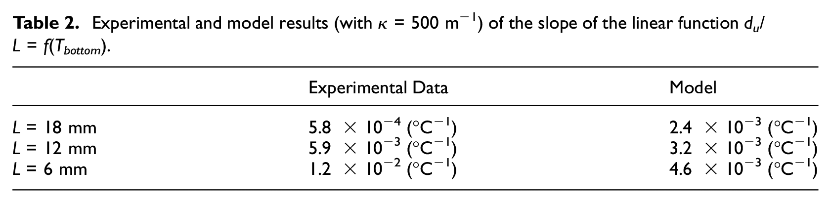
If one performs a linear regression analysis for the experimental and model results for Tb between −5°C and 50°C (as performed in Vali et al. 4 for the experimental lower layer depths), one can see in Table 2 that the ‘sensitivity’ of du/L to the bottom temperature increases substantially as the liquid pool gets thinner. This is only ‘moderately’ captured by the model. It is important to note that equation (16) is not a linear but a logarithmic function. Nevertheless, the behaviour of the proposed expression for the range of values examined in this work is ‘nearly’ linear.
Experimental and model results (with κ = 500 m−1) of the slope of the linear function du/L = f(Tbottom).
The results displayed in Figure 5 (right sub-figures) show that Nu i increases with increasing bottom temperature, Tb, because of the increased upper layer depth (as shown on the left sub-figures), which is directly proportional to Nu i , as can be seen from the combination of equations (9) and (10). Furthermore, the temperature difference (not shown here) used in equation (9) does also increase with increasing bottom temperature, Tb. The right sub-figures in Figure 5 show also that Nu i increases with decreasing κ for similar reasons. Physically speaking, a lower κ corresponds to more in-depth penetration and thus, more pronounced convective motion. Finally, it is important to mention that the thinner the pool the lower the value of Nu i because of the reduced buoyancy-induced instability, which is in line with the earlier observation that most likely another mechanism becomes dominant, that is, surface tension–driven convection.
An attempt to ‘improve’ the current model results is provided in the following sub-section.
Method 2 based on the radiative heat balance
The development of the ‘radiative heat balance integral method’ has started from the observation that using the method illustrated in Figure 4 for the determination of the upper layer depth, in combination with the constraint that the peak temperature does not exceed the boiling point, inevitably leads to an average upper layer temperature that is significantly below the boiling point. Therefore, the idea is to still use the temperature profile provided by equation (14) and find the ‘optimal’ combination of Ts and du that gives an average upper layer temperature that is equal to the boiling point
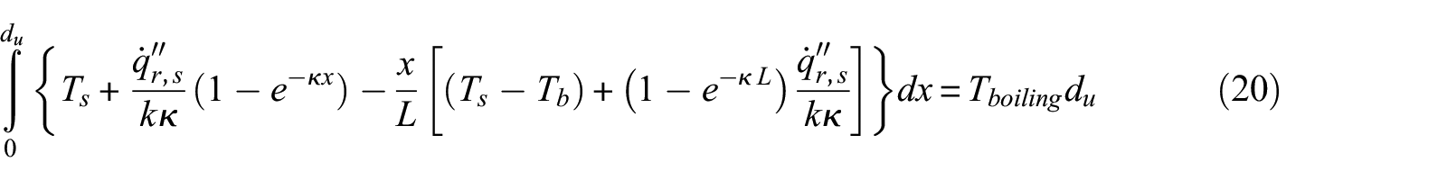
An example of the ‘transformation’ of an ‘inverse temperature profile’ into the thermal structure described earlier in the article is given in Figure 6.
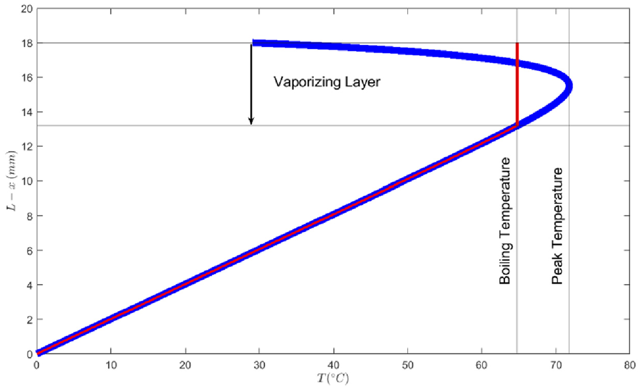
Liquid temperature profile for a case examined in Vali et al.
4
with the following parameters: Ts = 29.1°C, Tb = 0°C, κ = 1000 m−1,
A graphical representation of the optimization procedure is displayed in Figure 7. Such optimization procedure lies on a root-finding algorithm to find the values of du and Ts which make the curve of the function f (du) = I – Tboiling du tangent with f (du) = 0 at the depth of the vaporizing (boiling) layer. It is very important to recall here that, similarly to method 1, Ts is an unknown problem that does not represent the actual BC at the liquid surface (which is the radiative heat flux). The difference with method 1 is that the peak temperature is not fixed to Tboiling but is an output of the algorithm. As shown in Figure 6, the peak temperature exceeds the boiling temperature so that the average temperature across the upper layer becomes equal to Tboiling. To sum up, the inputs are
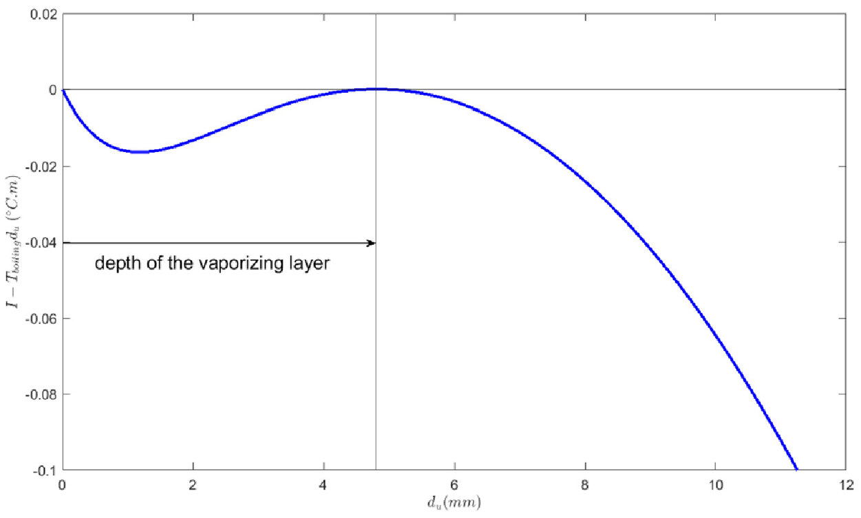
A graphical representation of the optimization procedure used in method 2 for the same case displayed in Figure 6. The parameter I in the y-axis represents the right-hand side in equation (20).
One can state that, based on the argument developed in the first method, below the locus of the peak temperature in the profile provided by equation (14) (see blue thick line in Figure 6), there are no instabilities that would lead to convective motion and mixing. Nevertheless, it is important to bear in mind that the interface located at the position provided by
Figure 8(a), (c) and (e) shows that a value of κ = 1000 m−1 gives an overall good agreement with the experimental data for the non-dimensional upper layer depth, du/L, particularly for L = 12 mm. For L = 18 mm, the upper layer depth is overpredicted with κ = 1000 m−1 for Tb > 30°C. For L = 6 mm and Tb < 35°C, the absorption coefficient had to be increased to 2000 and even 5000 m−1 to have a good agreement with the experimental data. Nevertheless, as mentioned for method 1, this can be attributed to the fact that surface tension–driven convection, which becomes important in thin pools, is not considered in the current modelling. The main difference in the upper layer depth results between the two methods is in the value of κ which gives the overall best results: κ = 500 m−1 for method 1 and κ = 1000 m−1 for method 2.
Regarding the predictions for Nu i , the overall same trends are observed for method 2 as for method 1. A more detailed comparison is provided and discussed in the next section.
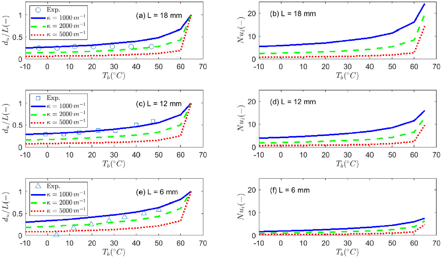
Results with method 2 for a 90-mm-diameter methanol pool fire as a function of the bottom layer temperature. A comparison between the experimental measurements 4 and numerical predictions of the non-dimensional upper layer depth (left) and predicted Nu i (right).
Before comparing the method proposed in Vali et al.
4
with the two methods proposed in this work, a sensitivity analysis has been carried out on the radiative heat flux, which was taken in the calculations above as
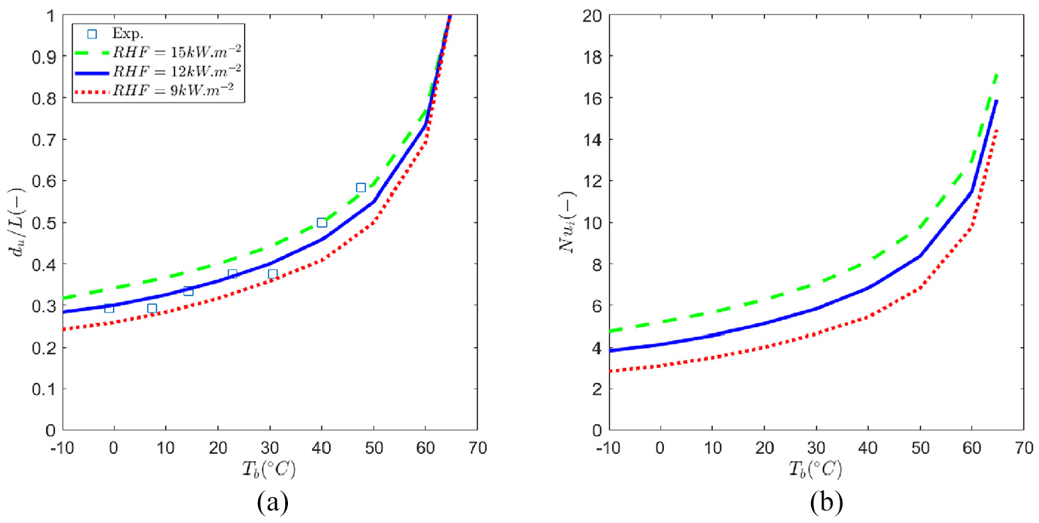
Influence of the radiative heat flux on the predictions (using method 2) of (a) the non-dimensional upper layer depth and (b) the Nusselt number, Nu i , for the 90-mm-diameter methanol pool fire with L = 12 mm and κ = 1000 m−1.
A comparative analysis
In order to compare the two methods proposed here with the approach proposed in Sikanen and Hostikka, 3 let us consider the case of a methanol liquid fuel subjected to a radiative heat flux of 20 kW/m2 (at its upper surface) with depths ranging from 0.005 to 0.200 m. The temperature at the bottom boundary is assumed to take the value of Tb = 20°C.
The Nusselt numbers displayed in Figure 10(a) show significant deviations between the method proposed in this work and the method developed in Sikanen and Hostikka. 3 The deviations increase with increased liquid depth. This is caused by the difference in depth over which the in-depth radiative source term is distributed, as visualized by comparing Figures 2 and 3. This is also shown in Figure 10(b) where the upper layer depth, du, predicted by the two methods is significantly lower than the overall liquid depth, L, used as a length scale in equation (6). When comparing the results between method 1 and method 2, it is important to bear in mind that the same absorption coefficient of κ = 1000 m−1 has been used here. Based on the sensitivity analysis carried out earlier in this work on κ for the two methods, we recall here that for the same value of κ, method 1 predicts lower values of du, as confirmed here in Figure 10(b). This is the main reason for the discrepancies between method 1 and method 2 in the values of Nu i , the calculated temperature differences used in equation (9) (and not shown here) are rather similar.
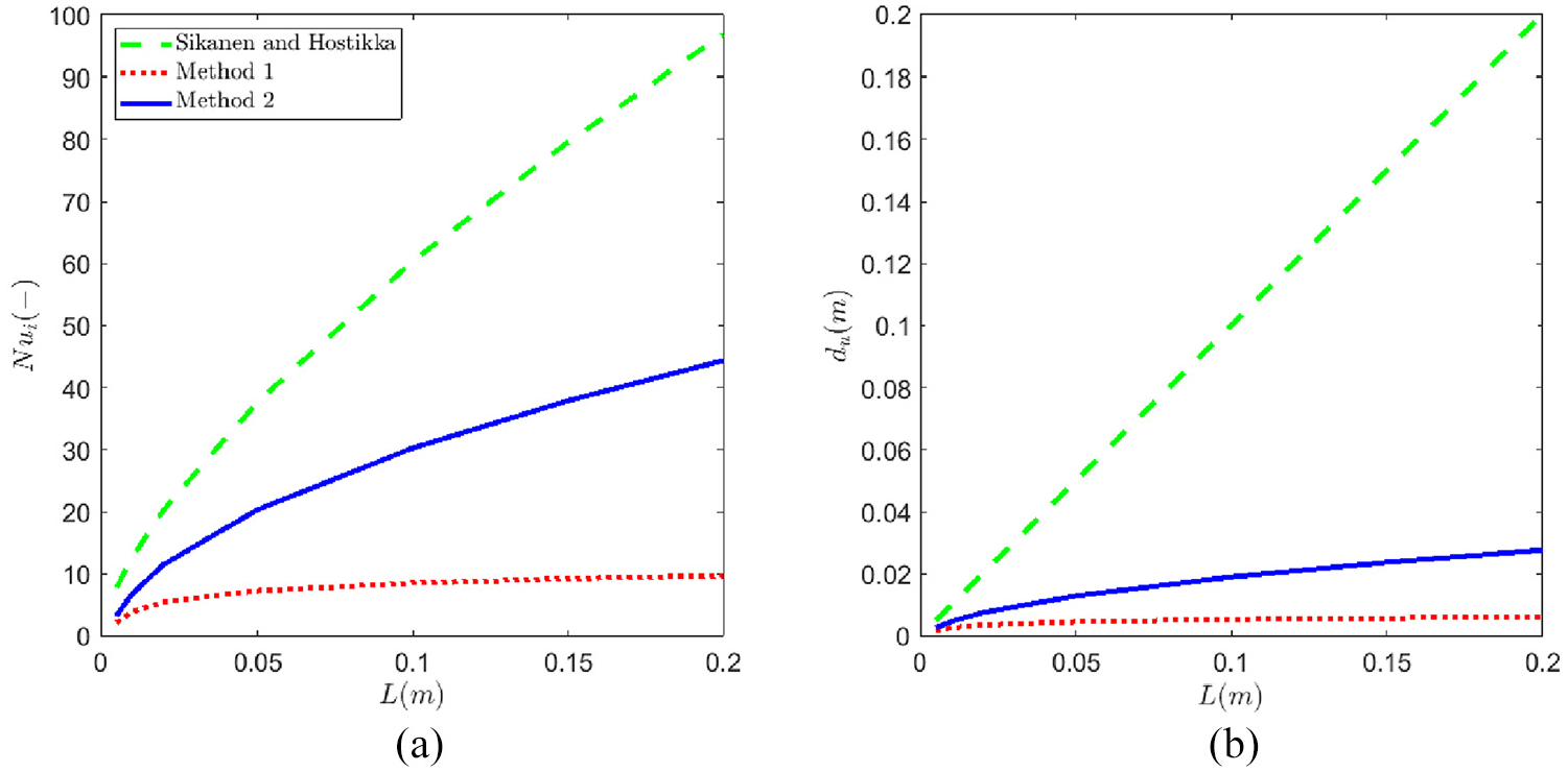
A comparison between the approach proposed in Sikanen and Hostikka
3
and the two methods developed in this work. The liquid fuel is methanol, Tb = 20°C, κ = 1000 m−1 and
At this stage, it is difficult to be assertive with respect to the ‘validity’ of the calculated Nusselt numbers or the ‘performance’ of one calculation procedure over the other. More detailed experimental measurements are needed for this matter. The same comment holds for an important fuel property used herein, namely, the effective absorption coefficient, κ. Nevertheless, in the meantime, one could implement the theoretical approach described herein in the simulation of pool fires and assess its influence on global quantities such as the peak (and steady) heat release rate and the time to reach the peak (or the steady state).
Foreseen applications in numerical modelling
It is envisioned that the theoretical and analytical work developed here can serve as a sub-model in the modelling of the liquid heat-up in the case of a pool fire. More specifically, the 1D Fourier’s equation would read

Besides the calculation procedure of keff, there are two differences with the work described in Sikanen and Hostikka. 3 The first one is that the radiative heat flux would exclusively be used as a BC for the upper (thermally thin) layer and not as a source term in equation (1). The second difference between equations (1) and (21) is related to the treatment of in-depth radiation as one can visualize by comparing Figures (2) and (3). The increased conductivity in equation (21) is only applied to the upper layer. Equation (20) plays, in this regard, a key role in the calculation procedure.
An alternative to solving equation (21) would be to use the concept of two-zone modelling for heat transfer in the liquid phase. In such two-zone modelling framework, the volume of the two ‘control volumes’ would be known thanks to equations (16) or (20). A remaining aspect to be modelled (regarding heat transfer) is the heat exchange between the two zones (i.e. the upper and the lower layers), which is out of scope of this article.
Both ways of liquid heat-up modelling described above (i.e. 1D Fourier’s equation or two-zone modelling) can be coupled to gas phase modelling in CFD simulations with the intent of saving computational resources without compromising the accuracy of the simulations, which is, in any case, not ‘guaranteed’ even if the full Navier–Stokes equations in the liquid phase are solved.
Conclusion
Fully predictive numerical simulations of liquid pool fires require a full and accurate coupling between the gas phase and the liquid phase. While extensive research work has been (and is still being) carried out on the gas phase, focusing on aspects such as combustion, soot and thermal radiation, an accurate treatment of the liquid heat-up is still lacking.
The purpose of this work has been to explore a methodology for the modelling of the liquid phase that would not require extensive and prohibitive computational resources to perform ‘practical’ fire dynamics simulations.
The theoretical and analytical work carried out herein is based on the assumption that in-depth radiation generates hydrodynamic (Rayleigh–Bénard) instabilities leading to enhanced convective heat transfer over a limited upper layer depth of the liquid. The analytical expression that has been derived for the upper layer depth (under the aforementioned assumption) has been compared against available experimental data for a 9-cm-diameter methanol steady-state pool fire and three different liquid depths (18, 12 and 6 mm), maintaining the bottom boundary temperature at several values between −10°C and 50°C. Encouraging results have been obtained in terms of qualitative variation of du with the bottom layer temperature (or temperature difference between top and bottom) and the overall liquid depth. However, this method does not ensure a well-mixed upper layer at a temperature near the boiling point, as suggested by the experimental data. Subsequently, an improvement is proposed based on a radiative heat balance integral method. In addition to the above, a novel methodology is developed for the calculation of the ‘effective’ thermal conductivity as a means to circumvent detailed calculations of heat transfer within the liquid.
The theoretical and analytical work presented in this article requires further validation by considering a wider range of conditions (e.g. fuel type and pool diameter). It has the potential to strongly support CFD simulations that rely on (1) a 1D heat transfer treatment of the liquid using a discretized Fourier’s equation (as in Sikanen and Hostikka 3 ) or (2) a novel treatment of the liquid heat-up using a two-zone modelling in an analogous way to what is commonly done about smoke stratification in the early stages of an enclosure fire.
Footnotes
Declaration of conflicting interests
The author(s) declared no potential conflicts of interest with respect to the research, authorship and/or publication of this article.
Funding
The author(s) disclosed receipt of the following financial support for the research, authorship, and/or publication of this article: This work was supported by Bel V [Scientific Research Agreement A18/TT/0674, Amendment N°1, Reference A19/TT/1632].