
Abstract
Studies quantifying value added of transit often cannot differentiate whether the premiums are transit effects or location effects. Limited studies have examined the timing of value added. Using before and after data, this study explores the impact of the Green Line LRT on housing sales prices. Compared to the studied period before its funding announcement, its announcement increased housing values by $9.2/sq ft and its commencement increased sales prices by $13.7/sq ft. Further analyses show that housing value appreciation actually occurred after the announcement but before the commencement. Thus, using the right timing of value added is critical for value capture programs and benefit–cost analysis.
Introduction
Many regions in the United States have shown a great interest in rail transit investments to mitigate the growth in traffic congestion. However, rail transit tends to have a large price tag and requires substantial subsidies from all levels of governments (O’Toole 2010). To justify the subsidies, transit planners often claim that rail transit has the potential to facilitate transit-oriented development and stimulate economic development, such as property value uplift. Not surprisingly, many scholars have examined the value added of rail transit (Pan et al. 2014; Jun 2012; Weinberger 2001). These studies offer important insights to value capture programs and rail transit planning (Smith and Gihring 2006; Gihring 2001).
Hedonic pricing models are often used to evaluate the impact of transit infrastructures on property values (Higgins and Kanaroglou 2016). Most studies examine the value uplift after the operation of transit and hence are weak in inferring whether the premium associated with transit proximity is due to transit itself or to the highly accessible locations where transit stops are located (Ko and Cao 2013). This points to longitudinal models to explore the value added of transit infrastructure (Smith and Gihring 2006). Moreover, for the sake of benefit–cost analysis or value capture, transit planners are interested in the timing of the value uplift, which “is far from clear” (Mulley and Tsai 2016, 16). This study aims to fill the gaps.
Using tax parcel data, this study applies difference-in-difference (DID) models to assess the impacts of the Green Line light rail transit (LRT) on sales prices of single-family houses (including detached houses or attached houses as in duplexes, triplexes, and townhouses) in the city of St. Paul, Minnesota. Based upon hedonic pricing models, it aims to answer the following two research questions: To what extent did the Green Line LRT increase housing values? When did the value uplift occur? The announcement of the full funding grant agreement (FFGA) on April 26, 2011, and the commencement of the Green Line on June 14, 2014, were chosen as key time points to test when the value uplift occurred. We also tested the changes in sales prices from 2008 to 2016 to illustrate a holistic picture of the housing market along the Green Line corridor.
This article is organized as follows: The next section reviews the gaps in the literature and critiques the studies that focus on the timing of transit impacts. the third section introduces research design, the data and variables, and the method of hedonic difference-in-difference models. Model results are presented in the fourth section. The last section replicates the answers to the two central questions and discusses the implications to planning practice.
Literature Review
A large number of studies have evaluated the impacts of transit investments on property values (e.g., Duncan 2011; Hess and Almeida 2007; Diao 2014; Cao and Hough 2008). Transit investments improve the accessibility of transit station areas and hence may uplift the demand for such locations. On the other hand, when a location is very close to the transit line, it may be negatively affected because of transit-related nuisances such as noise and pollution. The observed impacts of transit infrastructure on housing values are combined effects of both accessibility and nuisance (Chen, Rufolo, and Dueker 1998). Taken altogether, most studies concluded a positive premium associated with the proximity to transit infrastructure although there are some mixed results (Knowles and Ferbrache 2015; Debrezion, Pels, and Rietveld 2007). Further, value uplift shows a great variation. In a meta-analysis of 23 studies on rail transit, Mohammad et al. (2013) concluded that the variation results from land use type, transit type, transit system maturity, distance to rail stations, and so on.
However, many studies regarding transit and property values fall short in the following two aspects. First, before–after studies are needed to differentiate transit effects from location effects (Ko and Cao 2013). Previous studies often use only data from after the opening of transit to examine its impact on property values (Xu and Zhang 2016; Zhong and Li 2016). Transit stations are often located at major arterial intersections or close to key activity centers and as such residents are willing to pay a premium for the accessibility. Thus, the positive impacts of proximity to transit stations may be a proxy for the effects of accessible location, regardless of the presence of transit service (Ko and Cao 2013). Accordingly, a before–after analysis is necessary to examine whether the premium was present before its opening and whether the change in the premium is significant after its opening (Ko and Cao 2013). Further, scholars should rule out the possibility that the premium changes are due to the trend of the housing market in the region such as rising or declining economy (Rodríguez and Mojica 2009). Therefore, control areas are desirable to help cancel out the confounding effects of unobserved third-party variables on housing values.
Second, most studies focus on the impacts of transit investments after transit opens, although the impacts may occur before its commencement (Cao and Porter-Nelson 2016; Mulley and Tsai 2016). If the latter is true, the benefits of transit investments will be underestimated in two ways. The value added before its commencement are not considered in the calculation of benefits. And, the premium obtained through a before–after analysis is undervalued because property values before its opening have included the impacts of transit investments. Therefore, it is critical to identify when transit investments begin to increase property values (Mulley and Tsai 2016).
Previous studies have assessed the impacts of transit infrastructure before its operation, but the effort is rather limited. Bae, Jun, and Park (2003) explored the impacts of a subway in Seoul on residential property values. They first conducted four separate cross-sectional hedonic pricing models: for the years of subway announcement, one year during construction, at subway commencement, and again three years after its opening. For the first three time points, they found that the distance to the subway is negatively associated with property values (i.e., proximity to subway has a positive premium), but the relationship is insignificant for the last time point. They concluded that the subway has impacts only before its opening. However, as Ko and Cao (2013) argued, a before–after analysis is more desirable than four cross-sectional models, because it is unknown whether the impacts are due to the subway or the location of the subway stations. Bae, Jun, and Park (2003) also developed a pooled model with the data from the four years. Because they did not consider the interactive terms between the distance to subway stations and the indicators of different years as a DID model specifies, the pooled model cannot answer the aforementioned question.
Knaap, Ding, and Hopkins (2001) examined the impacts of the announcement of Tri-Met LRT in Portland on sales prices of vacant residential parcels in Washington County, Oregon. Based on the results of DID models, they found that after the announcement, sales prices of parcels within half a mile of planned stations increased by 36 percent. Besides control variables, a classic DID model includes three variables: a dummy indicating a property is within the impact area, a dummy indicating a property is sold after the key date, and an interactive term between the two dummy variables (please refer to the methodology section for the DID model). However, Knaap, Ding, and Hopkins (2001) omitted the temporal dummy variable, which may lead to a biased estimate of the interactive term (Brambor, Clark, and Golder 2006). Although they controlled for the month that a parcel was sold, they assumed an unlikely linear relationship between the month and sales prices.
Golub, Guhathakurta, and Sollapuram (2012) employed DID models to evaluate the impacts of LRT in Phoenix on property values from conception to operation. They concluded that the proximity to LRT stations lifted values of single-family homes, homes in multifamily structures, commercial properties, and vacant lands, although some values added are insignificant. For single-family homes, it appeared that the premium of the proximity has increased during different periods in the planning and construction process. Mulley and Tsai (2016) also used a DID model to assess the impacts of a bus rapid transit system in Sydney. They found that compared to properties sold two years before its operation, property values increased by about 11 percent, significant at the 0.1 level, during the first two years of opening, but that during the subsequent two years, the impact became insignificant, though positive. However, they did not illustrate whether the impact occurred before its commencement as Golub, Guhathakurta, and Sollapuram (2012) did.
McMillen and McDonald (2004) analyzed repeat-sales data within 1.5 miles of the Midway Rapid Transit line in Chicago and concluded that the announcement of the line affected single-family housing prices. Their model is a special case of the DID models as it uses the data of properties that are sold more than once. The repeat-sales estimates are more effective to account for the influence of time-invariant attributes than the DID models. However, McMillen and McDonald (2004) also acknowledged that repeat-sales are only a small subset of the whole transaction data and the repeat-sales estimates may be subject to some selection bias. Using 912 station-area residential properties sold more than once between 1971 and 1990, Gatzlaff and Smith (1993) explored the impacts of Miami Metrorail on housing prices. They first computed and compared repeat-sales indices between the Miami region and Metrorail station areas and suggested that the Metrorail announcement had an effect. Then they examined the influences of the announcement dummy, distance to rail stations, and their interactive term on housing prices in hedonic models and concluded that the announcement of Miami Metrorail marginally affected the sales prices of houses located in north stations but not in south stations.
Some studies have applied DID models to explore the effects of LRT in the Twin Cities, although dependent variables are not property values. Hurst and West (2014) examined the impacts of the Blue Line LRT on changes in land use before construction, during construction, and after commencement. They found a small difference between construction periods and operation periods. Further, the LRT seems to impact single-family and industrial properties, but does not influence vacant land, multifamily, and commercial properties. This small difference is not surprising, because market forces are insufficient to produce land use change and would require amendments or changes to zoning regulations. Alternatively, Cao and Porter-Nelson (2016) evaluated the effects of two key announcements of the Green Line LRT on building permits. They found that the announcement of preliminary engineering does not have positive impacts on building permits in the city of St. Paul, whereas the FFGA announcement increases both the number of and value of building permits. However, they did not evaluate the impacts after its opening, because the Green Line did not open yet when the empirical analysis was completed.
The authors of this study choose major arterial corridors in St. Paul as controls to the Green Line corridor by adapting the research design of Cao and Porter-Nelson (2016). It applies DID models to assess the impacts of the Green Line on housing values during the planning process and determine the timing of value uplift. It is worth noting that Ko (2016) also studied the value added of the Green Line. Ko developed spatial hedonic models on pooled data during 2009–2015 and concluded that proximity to LRT stations has positive associations with sales prices of single-family and multifamily housing. Ko stated that the significance of the interactive term between station proximity variables and each of five dummy variables of years (indicating 2010, 2011, . . . 2014) was tested and found that the interactive term with 2012 was significant. Then the author concluded that value uplift occurred in 2012. However, the model results were not shown in the article. Furthermore, it seems that Ko compared the properties sold between 2009 and 2011 and those sold between 2012 and 2015. Because the FFGA was announced in April 2011 and the Green Line commenced in June 2014, Ko cannot determine whether the value added was due to the FFGA announcement or the commencement of the Green Line. This study aims to address the question as well as to show the trend of housing prices over time.
Methodology
Research Design
The following project facts provide the context for this research. The Metropolitan Council’s Central Corridor Project Facts show that the 11-mile Metro Green Line connects downtown Minneapolis and downtown St. Paul along the University of Minnesota and University Avenue. It was initially called Central Corridor LRT and then branded as Green Line LRT. It has eighteen new stations (fourteen in St. Paul) and overlaps with the Hiawatha Blue Line at five stations in Downtown Minneapolis. The Green Line cost $957 million, and half was federally funded. Construction began at downtown St. Paul and the University of Minnesota campus in late 2010 and heavy construction ended in 2013. LRT service began on June 14, 2014, with a projected ridership of 41,000 per weekday by 2030. According to the data released by Metro Transit, the ridership was more than 45,000 in September 2015.
This study adopts a before–after research design and compares property values of treatment and control corridors. The treatment is the Central Corridor where the Green Line operates. The Green Line runs in both Minneapolis and St. Paul. Minneapolis is located in Hennepin County and St. Paul is located in Ramsey County. Because the tax parcel data in the two cities are compiled by different counties, property attributes are inconsistent between the two data sets. For example, the number of bedrooms, the number of family rooms, and the number of stories are available in the parcel data for St. Paul, but not available for Minneapolis. Therefore, this study focuses on only the segment of the Green Line in the city of St. Paul (referred as the Green Line for simplicity). The Central Corridor is mixed-use areas with many small ethnic businesses. The controls are three corridors (Snelling Avenue, West 7th Street, and Payne-Maryland Avenue) in St. Paul (Figure 1). Control corridors were recommended by local planners because all three corridors are basically mixed-use and lie along major arterials, and have the most frequent level of transit services in St. Paul and were planned to be developed as an arterial bus rapid transit (BRT) network.
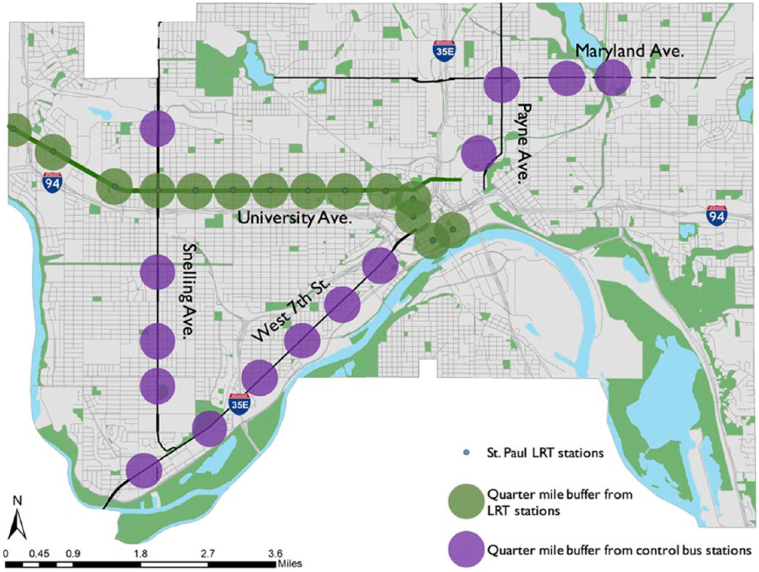
Station/stop areas of the Green Line light rail transit corridor and control corridors in the city of St. Paul.
This study analyzes the impact of two key time points: the FFGA announcement and opening. They represent significant progress toward the planning and operation of the Green Line. The FFGA announcement on April 26, 2011, indicated that the Federal Transit Administration was committed to building and funding half of the Green Line. The FFGA was a key planning process milestone. Cao and Porter-Nelson (2016) concluded that the FFGA announcement positively affected building activities along the Green Line.
Data and Variables
This research is based on tax parcel data maintained by the Ramsey County Assessor’s office. In this study, normalized sales price, sales price per square foot, is used as the dependent variable. Because the living areas of apartments and mixed-use residential properties are missing in the parcel data, they are excluded from the analysis. Further, condominiums are available in the Green Line Corridor but not in the control corridors; thus, they are also excluded. So we include the sale of single-family detached houses, two/three-family houses, and townhouses. We also remove ten outliers based on the results of the Grubb’s test. Since the FFGA was announced in April 2011, we consider properties sold from 2008 to September 2016 (when the data were assembled for the revision) to capture transactions before the FFGA, after the FFGA, and after the operation. Table 1 describes the variables tested in this study. The location variables were computed using ArcGIS. All other variables were obtained from the tax parcel data.
Variable Description.

Table 2 illustrates the average sales prices over years in the treatment and control corridors. The properties in the control corridors are more expensive than those in the treatment corridor. A few notable differences between the two corridors over time were that (1) sales prices in the treatment corridor increased substantially from 2011 to 2012, whereas they decreased slightly in the control corridors; and (2) sales prices in the treatment corridor increased more than 50 percent from 2012 to 2014, but grew about 20 percent in the control corridors during the same period. These differences seem to imply the effect of the FFGA announcement on housing values. However, the effect of commencement is less clear. Multivariate analysis will be used to test the influences of the Green Line over time.
Housing Market along the Green Line and Control Corridors.
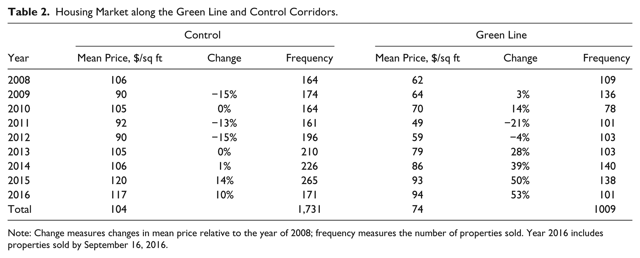
Note: Change measures changes in mean price relative to the year of 2008; frequency measures the number of properties sold. Year 2016 includes properties sold by September 16, 2016.
Modeling Approach
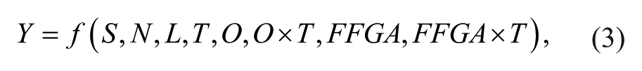
Hedonic pricing models are often used in the literature to quantify the impact of transit investments on property values. The rationale is that when an individual purchases a house, the buyer pays for a bundle of attributes associated with the house (Rosen 1974). The attributes include, but are not limited to, structure, neighborhood, and location characteristics of the house. Hedonic pricing models disentangle the implicit prices of these attributes. Accordingly, a hedonic model can be expressed as (subscripts are suppressed for simplicity)
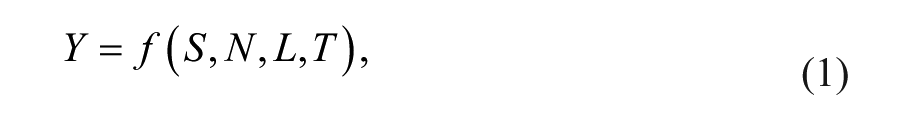
where Y is the sales price per square foot of a house, S includes a list of structural attributes, N contains a list of neighborhood characteristics, L constitutes a list of location attributes, and T is a dummy variable indicating the house is located within a specific distance of LRT stations, that is, treatment, catchment, or impact areas. We distinguish proximity to LRT from other location characteristics because of the purpose of this study.
A before–after analysis is necessary to distinguish whether the coefficient of proximity to LRT indicates an LRT effect or a location effect, as discussed in the literature review. Accordingly, the hedonic model requires an additional dummy variable O, which indicates whether the house is sold after the opening of the Green Line. To illustrate the concept of a DID model, equation 2 shows an example model with control variables, two base variables, and one interactive term.
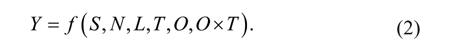
If the interactive term, O×T, is insignificant, the coefficient of the dummy variable T measures the effect of housing location (either in the treatment corridor or control corridors) on housing prices but it is not related to the opening of the Green Line LRT. In this study, we assume that the effect is uniformly distributed within the treatment areas as we do not test the price impact of the distance to LRT stations. We expect it to be negative because houses in the control corridors are more expensive than those in the treatment corridor. Similarly, the coefficient of the dummy variable O measures the temporal trend of the regional housing market before and after the LRT opening but it is not related to housing location. By contrast, the coefficient of the interactive term between the dummy of proximity to LRT and the opening dummy, O×T, indicates the effect of the LRT opening on housing price. This interactive term is our policy variable of interest, consistent with Billings, Leland, and Swindell (2011) and Hurst and West (2014). That is, because we test the timing of value added by LRT, we need to test the coefficients of the interactive terms between proximity to LRT and each of the temporal dummy variables described below. In this study, we first test the impacts of two key time points of the Green Line: FFGA and opening, as informed by Cao and Porter-Nelson (2016). We further test the impacts of each calendar year. The two tests are illustrated in equations 3 and 4, respectively.
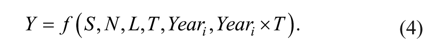
In equation 4, we further split the year of 2011 into two dummy variables to indicate the period before the FFGA and the period after the FFGA. Similarly, we split 2014 to indicate the periods before and after the commencement of the Green Line.
Fixed effect regression model with robust error is used to estimate equations 3 and 4. Because houses located in the same station area may share some common characteristics, fixed effect models are adopted to address the spatial dependency. The models are developed in Stata 14.0. We test all control variables in Table 1 and keep those significant at the 0.1 level to obtain parsimonious models. The dummy variables for proximity to LRT, time, and their interactions are kept in the models no matter whether they are significant, because they are the key variables of interest.
Results
Table 3 presents the two models associated with equations 3 and 4. Both models have the same set of significant control variables. In particular, two/three-family houses and townhouses have lower sales prices per square foot than single-family detached houses. The number of stories and the total number of rooms have negative associations with sales price per square foot. It is more expensive to build a one-story house than a two-story house of the same size because in the one-story house all living areas require a foundation. So a one-story house tends to have a higher sales price than a two-story house on a per-square-foot basis. Further, people often prefer an open floor plan with large rooms. 1 For houses with the same size, more rooms might have a lower sales price per square foot than fewer rooms. The presence of a garage is positively associated with sales price per square foot (housing values thereafter for simplicity). The year the building was built has a positive association with housing values (i.e., newer houses tend to have higher prices). All of these structural characteristics are consistent with our expectations. The distance to downtown St. Paul is also significant. The farther a house is from the downtown, the higher its value is. This makes sense because downtown St. Paul is surrounded by cheaper housing in terms of both total value and per-square-foot value (verified in the data). All else equal, associated with 1-km increase in the distance to downtown St. Paul, housing values increased by $15.5/sq ft, on average.
Fixed Effect Models for Housing Sales Price.
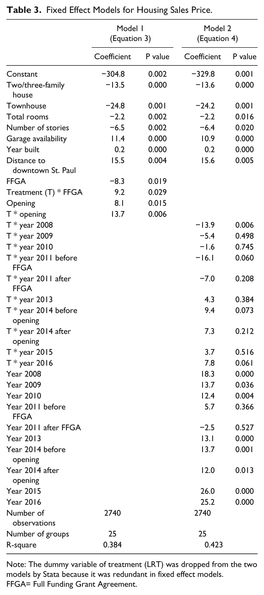
Note: The dummy variable of treatment (LRT) was dropped from the two models by Stata because it was redundant in fixed effect models. FFGA= Full Funding Grant Agreement.
In model 1, the two time dummy variables (the FFGA announcement and LRT opening) are significant. The FFGA announcement has a negative coefficient, but this does not mean that housing values in the LRT corridor decreased after the FFGA announcement. When the interactive effect is significant, explaining the unconditional effect of the time dummy is misleading, because its effect depends on the level of the other variable (Seltman 2015; Brambor, Clark, and Golder 2006). Since the interactive term between FFGA and T is significantly positive, the two coefficients jointly indicate that the values of houses in the control corridors decreased after the FFGA announcement whereas the values of houses in the LRT corridor grew after the announcement. For an illustrative purpose (as we did not consider the impacts of other variables significant in model 1), Figure 2 shows the relationships among the LRT, the FFGA announcement, and housing value.
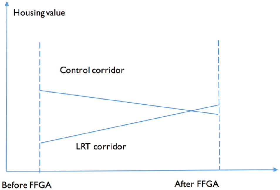
The relationships among LRT, FFGA, and housing values.
Now let us turn to the interactive terms. In model 1, the reference time period is before the FFGA announcement and the coefficient of T*FFGA is $9.2/sq ft. Therefore, compared to the housing values before the FFGA announcement, the announcement increased housing values by $9.2/sq ft. Similarly, the housing values after the opening of the Green Line was $13.7/sq ft than those before the FFGA announcement. These findings substantiate the capacity of LRT investments in boosting housing values. Further, the impact appeared when the FFGA was announced, three years before the operation of LRT. This timing is consistent with the value added of the elevated line from downtown Chicago to Midway airport explored by McDonald and Osuji (1995). However, the opening of the Green Line did not seem to generate significant housing values beyond the FFGA announcement, because the difference between the coefficients of T*FFGA and T*opening is not statistically significant (the specific test result is not shown).
Figure 3 shows changes in housing values over time, which are associated with model 2. Because the reference period is 2012 in model 2, all changes are relative to the year of 2012 and the control corridors. Housing value differences between the LRT and control corridors in 2008 were $13.9/sq ft lower than those in 2012. Put another way, if houses in the LRT corridor was M dollars/sq ft cheaper than houses in the control corridors in 2012, houses in the LRT corridors would be $(13.9+M)/sq ft cheaper than houses in the control corridors in 2008. Housing values in the LRT corridor grew faster (or decreased slower) than those in the control corridors in 2009 and 2010. So housing value differences were getting similar among 2009, 2010, and 2012. Before the FFGA announcement in 2011, housing value differences were $16.1/sq ft lower than those in 2012. This coincided with the bottom of the housing market in the Twin Cities. The Central Corridor was hit particularly hard because many homes along the corridor were occupied by minority and low-income residents. However, after the announcement in 2011, housing value differences recovered by $9.1/sq ft, which was presumably due to the news that the Green Line was to be built. However, the improvement is not statistically significant (the specific test result is not shown). The momentum continued in 2012 with an additional improvement of $7.0/sq ft, which is not statistically significant. In 2013, housing value differences kept improving by $4.3/sq ft. In the first half of 2014 (before the commencement of the Green Line), housing value differences experienced another improvement of $5.1/sq ft. It is worth noting that although the LRT was not open during this period, the Metropolitan Council promoted the media appearance of the Green Line with a series of stories. Trains were tested on the tracks. Residents were aware of the upcoming LRT. These may contribute to the faster increase in housing values in the LRT corridor. In the rest of 2014 and 2015, housing value differences reversed somewhat, probably a correction to the housing market. In 2016, housing value differences improved again. Although the year-to-year changes of housing value differences during the whole studied period are not statistically significant, an uprising trend was observed after the FFGA announcement.
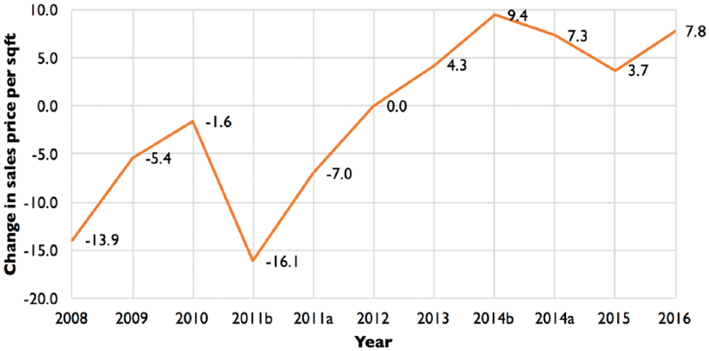
Changes of Housing Values in the LRT Corridor relative to the Control Corridors over Time.
Conclusions
A limited number of studies have explored the timing of value added by transit investments, although it has important implications for value capture and benefit–cost analysis. This study employed hedonic difference-in-difference models to quantify the impacts of the recently commenced Green Line LRT in St. Paul, MN, on sales prices of the houses within a quarter mile of stations and determine the timing of value uplift.
This study has a few limitations. The DID model can eliminate the influence of omitted time-invariant attributes (such as land use patterns and school quality) as long as their influences on housing values remain constant over time. However, it cannot address time-varying attributes such as unemployment rate during the economic recession and recovery. Unfortunately, the year-to-year data are not available at the small scale. Further, the DID model can control for the temporal trend of the regional housing market. However, the foreclosure crisis could be a potential confounding factor, because it was worse in the Green Line corridor than in the control corridors. The overrepresentation of low-income and minority individuals implies a high number of subprime mortgages in the Green Line corridor. After the housing market recovered, the positive change in housing sales prices could be more pronounced along the Green Line than in the control corridors. On the other hand, we attempted to drop more low-price houses. Although the value added reduces slightly in size, the trend over the year still holds. Further, this study focuses on the LRT segment in the city of St. Paul and does not capture the value added in the city of Minneapolis.
Nevertheless, this study offers insightful results. According to the results in model 1, compared to the studied period before the FFGA announcement of the Green Line, housing values increased by $9.2/sq ft after its announcement and $13.7/sq ft after its commencement. However, the difference between the funding announcement and the commencement is insignificant. Figure 3 illustrates the temporal trend of housing values in the Green Line corridor relative to the three control corridors and offers a more nuanced picture than the results in model 1. Overall, after the FFGA announcement, housing values kept increasing until its opening. Although none of the year-to-year increases are statistically significant, Figure 3 clearly shows that housing appreciation occurred before the opening of the Green Line and then remained stable after its opening. These findings substantiate that the Green Line LRT lifted the values of houses nearby, and that the value uplift occurred right after the funding for the line was confirmed. Therefore, the timing of value uplift should be carefully considered in the benefit–cost analysis of transit investments.
It is worth noting that some increases in housing values along the Green Line corridor should be attributable to policies and investments associated with the LRT, a secondary effect of LRT investments (Golub, Guhathakurta, and Sollapuram 2012). For instance, the city of St. Paul dedicated $13.5 million for streetscape improvements along the corridor, in addition to resurfacing University Avenue, and 85 percent of on-street parking spaces were removed (St. Paul 2015). Thus, both the appearance of the streets and pedestrian infrastructure improved compared to before. These plans enhanced neighborhood attractiveness and promoted the use of alternative means of transport. Furthermore, the zoning amendments implemented in April 2011 (St. Paul 2011) also increased the development potential of existing properties, which helped to uplift housing values. Therefore, proactive policies and plans related to LRT investments seem to help value capture, as well as neighborhood quality and sustainable mobility.
The sizable increase in housing values is good news for value capture programs. Higher property taxes associated with the value uplift help justify local government investments in transit infrastructure and provide additional revenues for other service investments in the city of St. Paul. The value added also brings fortune to home-owners along the Green Line corridor. This is particularly important because of the overrepresentation of low-income owners in the corridor. On the other hand, higher taxes may be an increased financial burden to existing home-owners. Also, the value uplift is likely to result in an increase in rental rates (Pollack, Bluestone, and Billingham 2010). Accordingly, some existing home-owners and renters could be displaced to other low-income and less accessible areas. If this is true, individuals may lose social ties within the neighborhood as well as access to ethnic services and employment opportunities. These will adversely affect the welfare of the individuals. Further, if lower-income households are displaced by higher-income counterparts, gentrified households may use transit less and drive more than the displaced households (Danyluk and Ley 2007). This will undermine the effect of rail transit on travel behavior, countering its original goal. The literature suggests that rail transit and associated transit-oriented development have the potential to stimulate gentrification (Jones and Ley 2016; Kahn 2007) and in some transit-friendly neighborhoods, affluent residents and choice riders outbid low-income residents and captive riders (Pollack, Bluestone, and Billingham 2010). On the other hand, Rayle (2015) stated that there is little evidence to support large-scale displacement caused by gentrification because no rigorous studies have been conducted to examine the connections between gentrification and displacement. In terms of the Green Line, we have not seen a study about gentrification and displacement and an exploration of the difference in travel behavior between displaced existing households and gentrified households, and the implications for planning practice. These issues merit further investigation.
Footnotes
Acknowledgements
Special thanks to Donna M. Drummond, director of planning of the city of Saint Paul, for her insights on the foreclosure crisis.
Declaration of Conflicting Interests
The author(s) declared no potential conflicts of interest with respect to the research, authorship, and/or publication of this article.
Funding
The author(s) disclosed receipt of the following financial support for the research, authorship, and/or publication of this article: The study was funded by the Center for Transportation Studies, University of Minnesota.