






Abstract
The point factor method of job evaluation is one of the most popular and enduring approaches to linking the market and internal value of jobs. Statistically, regression analysis is used to create a market line that allows the organization to predict the market value of its jobs using point scores that define the jobs’ internal values. While attention is given to the fact that the market line represents the statistically “best” option for predicting these market rates, overlooked is the fact that these predictions almost always differ from the jobs’ actual market rates. This article explores the impact of this prediction error in compensation planning. It uses data on 41 jobs to define a market line using simple regression and identify the errors associated with the line’s predicted market values. It provides methods for precisely defining the extent of this prediction error and for minimizing it. It also discusses the impact of this error on the interpretation of salary grades, and the need for policy on key compensation planning issues to minimize the negative impact of prediction error.
According to Kilgour, 1 after sorting through a variety of variable pay programs that delivered disappointing results during the Great Recession, organizations are now showing a renewed interest in job evaluation techniques that effectively link the market and internal values of their jobs. Courts 2 continue to reaffirm the importance of market rates as a defensible basis for unequal pay rates, and practically speaking it is impossible to ignore the internal value of many jobs when making pay decisions. 3 Hence, the ability to effectively link these two components of job value is important to compensation planning.
Point Factor Method
One of the most common techniques for linking the market and internal values of jobs is the point factor method. Essentially, this method evaluates the relationship between the
labor market values of jobs at a specific level of competitiveness, like the 50th percentile and
organization-specific internal values of these jobs, defined in terms of point scores.
The point factor method typically relies on a statistical technique known as regression analysis to define a line that allows organizations to predict the labor market values of their jobs (Y) given the jobs’ point scores (X). This line, referred to by Milkovich et al., 4 as the market line, has the general form.
In the context of this discussion,
For example, assume that for a particular job b0 equals $20,000, b1 = 55 and x1 = 700 points. In this example, the predicted market value for the job is $58,500.
The
Although it is possible to compute the formula of different market lines in order to model the relationship between the market and internal value of jobs, the formula for the market line returned with a regression analysis of the data has the distinct property of minimizing the aggregate difference between the actual market values of jobs included in the analysis and their predicted market values. Because of this important statistical property, the line is referred to as the “line of best fit” and this property is routinely referenced in discussions of the development of market lines using regression analysis. For example, in their discussions, Milkovich et al. points out that the regression line “smoothes large amounts of data while minimizing variations,” 5 Martocchio notes that regression analysis “finds the best-fitting line between two variables” 6 and Henderson points out that regression analysis “minimizes the sum of squares of the vertical deviations around the line.” 7
While market lines developed using regression analysis do represent lines of best fit, and do minimize the differences between the actual and predicted values of jobs, it is important to note that they do not eliminate such differences. Although, in theory, the actual and predicted values of jobs may be the same, in practice this is seldom the case. Consequently, organizations using regression analyses to develop market lines must contend with the fact that the predicted values of their jobs are almost always different from the jobs’ actual market values.
Once recognized, this raises significant pay issues. For example, how will organizations determine the differences between the predicted and actual values of their jobs? What can be done to reduce these differences? And how will organizations accommodate these differences when making pay decisions, like assigning jobs to the appropriate salary grades or paying for the appropriate level of performance?
The inaccuracy of predicted market values, or prediction error, is illustrated using data collected by me. After developing and defining a market line, methods are presented for evaluating its degree of prediction error, for reducing the prediction error and for accommodating it when developing salary grades.
Market Line Prediction Error
Database Development: The database used to illustrate market line prediction error includes jobs at a private university in the Midwest. The following methodology was used to develop labor market rates and point scores for the jobs used to develop the market line.
Market Rates: After meeting with key university administrators, 41 benchmark jobs were selected that effectively represented the university’s organizational structure, and decisions were made about the labor markets in which the organization had to effectively compete in order to attract and retain well-qualified employees for each benchmark job. Multiple sources of published pay data were then used to calculate the 50th percentile market value of each benchmark job, current as of an agreed-on compensation planning date.
Point Scores: The point scores used to measure the internal values of benchmark jobs to the university were developed using the following six-step methodology.
Step 1: Factor Identification
During Step 1, in-depth interviews were conducted with key staff during which eight factors were identified that, in their opinion, defined the relative value of jobs to the university. These included factors such as the
level of discretion and judgment required for routine job performance,
impact of routine job performance on the university’s mission and business objectives and
impact of routine job performance on the quality of student education.
Step 2: Factor Scoring Schemas
During Step 2, schemas were developed for each factor, so that when job content was matched against the written definition of a factor by the organization’s job evaluation committee, it produced a numeric value. For example, the first factor listed above included five different levels of discretion and judgment. For scoring purposes, the numeric value of the first level was 1, the numeric value of the second level was 2, the numeric value of the third level was 3 and so on. Hence, if the committee decided the content of a job was best described by the first level of discretion and judgment, it received a score of 1, and if the committee decided the job’s content was best described by the highest level of discretion and judgment, it received a score of 5.
Step 3: Evaluate Jobs
During Step 3, the organization’s job evaluation committee evaluated the content of each job against the written definitions of each factor and generated scores for the jobs based on the scoring schemas developed in Step 2.
Step 4: Determine Factor Weights
During Step 4, factor weights were developed and used to calculate each factor’s weighted point scores. A multiple regression analysis of the relationship between the 50th percentile market rates of benchmark jobs and the jobs’ factor scores was used to identify individual factor beta values (i.e., b1, b2, b3, b4 . . . b8) or slopes. Because one of the factors had a negative beta value, a decision was made to drop it from the analysis. The beta values of the remaining seven factors were then summed, and the proportion of the total beta value represented by an individual factor’s beta value was used as the factor’s weight.
For example, assume the sum of the betas for the remaining seven factors equaled .050 and the beta value for Factor 1 equaled .009. In this example, the weight for Factor 1 would equal 18%.
Step 5: Determine Weighted Factor Points
After determining factor weights, point schemas were developed for converting the range of scores possible for each factor to weighted point values fitted to a 1,000-point scale. The maximum point values for factors were determined by multiplying the factors’ weights by 1,000. For example, the factor describing jobs’ discretion and judgment had five levels, with scores ranging from 1 through 5. If this factor’s weight was 18%, then the point value of it highest score, 5, would be 180.
Point values for lower scores on a factor were determined by incremental reductions in the point value of its highest score. The size of these incremental reductions was determined by dividing the point value of the factor’s highest score by the number of factor levels. For example, since the factor describing jobs’ discretion and judgment had five levels, the incremental reductions in its maximum point value of 180 would be 36.
Using this approach, the scores of 1, 2, 3, 4 and 5 associated with the levels of this factor, in Step 2, would have corresponding weighted point values of 36, 72, 108, 144 and 180.
Step 6: Determine Total Weighted Points
After a point schema was developed for each of the remaining factors, a conversion table was developed that converted the job evaluation committee’s initial score for each factor on each job in Step 3 to its equivalent weighted point value. Then, the total weighted points for each job were calculated by summing the job’s weighted points on each factor.
Table 1 shows the resulting database that was used to develop a market line. It includes the 50th percentile market rate (Y) and total point score (X) for each of the 41 benchmark jobs included in the analysis, listed by job code.
Database.

Note.
Regression Analysis
To develop a market line, a simple regression analysis of the 50th percentile market rates (Y) and total point scores (X) of benchmark jobs was conducted. Figure 1 shows the results of the analysis.
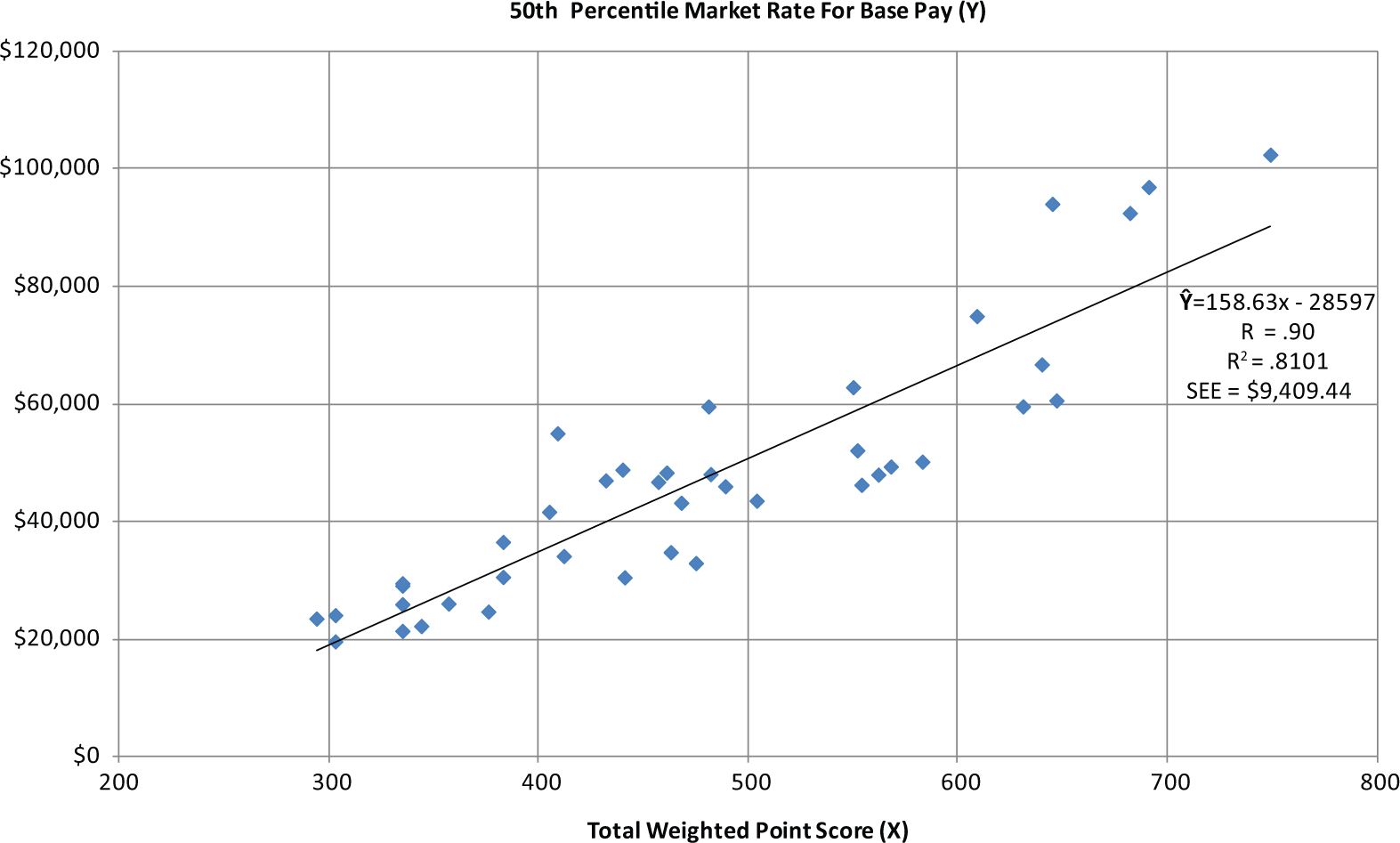
Regression analysis.
Unlike a multiple regression analysis, a
Market Line
In this analysis, the market line, or regression line of best fit, has the following formula.
In the context of this discussion,
For example, the database shown in Table 1 indicates that job code 21 was evaluated as having 583 total points. Using the above formula for the market line, the predicted 50th percentile market value for this job is approximately $63,884.
Prediction Error
The results of this regression analysis indicate a strong association between jobs’ market rates and total points (i.e., r = .90). However, despite this strong association, a substantial amount of variance in jobs’ market rates cannot be explained by their total points. In fact, the value of the coefficient of determination in this analysis (i.e., r2 = .81) indicates that
while 81% of the variance in the market rates of jobs is explained by their total point scores,
19% of that variance is not.
It is this remaining, unexplained variance that produces error when predicting the market rates of jobs. For example, although the market line’s predicted 50th percentile market rate for job code 21, with 583 total points, is $63,884, the database in Table 1 indicates the actual market rate for this job is $50,220. In short, the market line overstates the market value of this job by $13,664.
Table 2 illustrates the dimensions of the prediction error. It shows the actual market value, predicted market value and difference between these two values for each job included in the analysis. These data indicate that
Prediction Error.
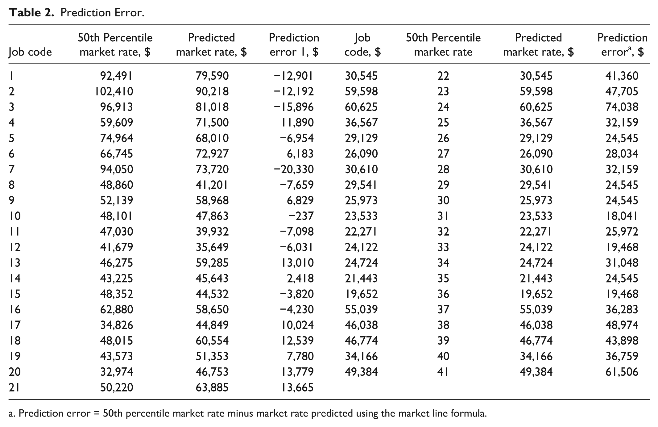
Prediction error = 50th percentile market rate minus market rate predicted using the market line formula.
none of the jobs’ predicted market values are the same as their actual market values and
the differences between jobs’ actual and predicted market values range from a low of $183 to a high of $18,756.
While different market lines have different ranges of prediction error, almost all have some prediction error that must be contended with when developing pay policy and corresponding salary structures.
Impact on Pay Policy and Salary Grades
Confidence in Predicted Market Values
Many organizations using the point factor approach to job evaluation construct salary grades around their market line’s predicted values for their jobs. 7 The predicted values are used to establish salary grade midpoints, and normative spreads above and below these midpoint values are then used to establish the salary grades’ minimum and maximum values. Generally, the normative spreads reflect the level of the job in the organization: The higher the level of the job, the wider the spread between the minimum and maximum values of the job’s salary grade is. According to Milkovich et al., 8 the normative range from the minimum to the maximum values of salary grades for
top management can vary from approximately 86% to 300%,
entry- to mid-level professionals and managerial jobs can vary from approximately 35% to 86% and
office and production workers can vary from approximately 11% to 35%.
When this approach is used to develop salary grades, its effectiveness depends on the accuracy of the market line’s predicted market values for jobs. For example, assume that the Midwestern university represented by these data has decided that it
wants to use salary grade midpoints to represent the value of completely satisfactory job performance,
will use the 50th percentile labor market values of its jobs to determine what their completely satisfactory performance is worth and
will use the market line generated by its point factor plan to predict these 50th percentile labor market values.
Based on this compensation strategy, the organization then develops what it anticipates will be a fully competitive pay policy. In general, the policy stipulates that
the midpoints of employees’ salary grades will reflect the 50th percentile market values of the jobs assigned to the grades,
the organization’s market line will be used to determine the 50th percentile market values of jobs and
employees who perform their jobs completely satisfactorily will receive a salary or wage equal to the midpoint values of their grades or increases in pay that move them closer to that target level of compensation, subject to appropriate budgetary constraints.
If the organization’s market line accurately predicts the 50th percentile market values of its jobs, there is every reason to believe that this pay policy will, in fact, be fully competitive. However, if it does not, a host of significant issues arise. For example, are employees who are currently being paid the midpoint values of their salary ranges receiving more or less than the labor market value of completely satisfactory performance in their jobs? How does the organization effectively link employees’ performance evaluations to adjustments in their base pay when it doesn’t know how market competitive their current pay level is? And how does the organization assess the budgetary implications of its pay policy when it doesn’t know how much of an adjustment in pay it needs to give employees in order to maintain the competitiveness of the plan?
Answers to these questions require information on the extent of error in market line predicted values. Consequently, it is important for the organization to know what the standard error of the market line’s estimates is, as well as the size of the prediction interval around the actual market values of specific jobs.
A
The
Standard Error of the Estimate
The standard error of the estimate measures the overall, or standard, difference between the market line’s predicted market values of jobs and the jobs’ actual market values, and it expresses this difference in terms of the depended variable (i.e., Y) used in the regression analysis. In the context of the present discussion, the value of standard error is expressed in terms of dollars.
Conceptually, the standard error of the estimate measures the scatter of data points about the market line. For example, an inspection of the scatter diagram in Figure 1 makes clear that if all of the data points in the diagram were on the market line, there would be no scatter. Under these conditions, there would be no difference between the predicted and actual market values of jobs, and the value of the estimated standard error would be 0. As the data points fall further and further from the market line, the differences between the predicted and actual values of jobs increase. As a result, the spread of data points about the market line increases, and the value of the standard error of the estimate increases.
The summary statistics listed in Figure 1 indicate that the standard error of the estimate (i.e., SEE) equals $9,409.44. This tells the organization that the standard difference between the actual 50th percentile market values of its jobs and the market line’s predicted market values of those jobs is $9,409.44. Table 3 provides details on the calculation of this key measure of prediction error using the database shown in Table 1.
Standard Error of the Estimate.

Note. Standard error of the estimate = √((∑(Y −
Prediction Intervals
Because the standard error of the estimate is a summary, or general, measure of prediction error, it does not provide direct information on the prediction error associated with specific jobs. For example, it does not tell the organization, with a given level of certainty, what the actual market rate is for a specific job with a specific total point score. This information is provided by the job’s prediction interval.
The formula for the prediction interval (PI) for a specific job is
In the context of this discussion,
For example, the analysis of the data discussed here indicates that the predicted 50th percentile market value of job code 21, with 583 points, is $63,884, with an estimated standard error of $9,409.44. Because this is an especially important job to the university represented by these data, it would like to know, with 90% certainty, what the job’s actual 50th percentile market value is. Based on the sample of 41 benchmark jobs used in the analysis, the organization may conclude with 90% certainty that this job’s actual market value is contained within the interval from $47,715.10 to $80,052.90.
Figure 2 shows, in more detail, the calculations required to compute this prediction interval. 9

Prediction interval calculations.
Impact on Salary Grades
When organizations use market lines to determine their salary grade midpoints, minimum grade values are set at lower pay levels to recognize less than completely satisfactory performance job while, at the same time, allowing organizations to attract qualified candidates who may not have substantial job-related experience. Alternatively, maximum grade values are set at higher pay levels to recognize outstanding job performance. As long as the midpoints of the salary grades accurately reflect the labor market values of the jobs in them, the grades’ interpretation is relatively straightforward. However, once prediction error is introduced this interpretation becomes more complex.
For example, the range between the lowest and highest values of the 90% prediction interval calculated for job code 21 with 583 is approximately 168%.
When the width of this range is compared with the normative salary grade widths identified earlier, the width of salary grades only for some top management jobs is enough to encompass the entire prediction interval for the completely satisfactory performance of this job. If the job were, instead, assigned to a more narrow salary grade, the university represented by these data could not conclude with 90% confidence that the incumbents in this job were being paid the market value of its completely satisfactory performance, even if their pay was equivalent to the maximum value of their salary grade and their job performance was judged to be outstanding.
In short, the utility of salary grades is substantially reduced when the entire prediction interval for the jobs assigned to them is not captured by the grade’s minimum and maximum values. To avoid this problem, organizations may decide to reduce the widths of the prediction intervals for selected jobs.
Reducing Prediction Interval Width
Generally, the narrower a prediction interval, the more likely it is to be entirely captured by a salary grade. Two major factors influence the interval’s width. One is the desired level of certainty. Other things being equal, the lower this level of certainty, the narrower the prediction interval is. Statistically, this is because lower levels of certainty are associated with smaller critical values of the t statistic (i.e., tcrit.). And an inspection of the formula for calculating prediction intervals shown in Figure 2 makes clear that these smaller values of tcrit. then result in narrower prediction intervals. Table 4 shows the general relationship between certainty, or probability level, and interval width at three different probability levels: that is, 60%, 80% and 90%.
Prediction Interval Widths. a

These data assume a job with 583 total points.
n = 41, degrees of freedom = n − 2, that is, 41 − 2 = 39.
Given the formula for calculating prediction intervals, one way for an organization to reduce width is to reduce the required level of certainty regarding a job’s true market value.
The other major factor influencing prediction interval width is the spread of data points about a market line. There is a positive correlation between this spread and the standard error of the estimate, so that reducing the former is associated with a reduction in the latter. A common approach to reducing spread is the elimination of outliers.
For example, even though there are no obvious outliers in the scatter diagram in Figure 1, the university may further reduce the scatter of data points around its market line by making the definition of outliers more restrictive. Using this approach, instead of eliminating all data points that were more than 3 standard deviations from the market line, as was the case in this analysis, the university could have chosen to remove all data points that were more than 2 standard deviations from the market line. If it had done this, some existing data points would be captured by this more restrictive definition of an outlier and removed from the analysis. The remaining data points would then “hug” the market line more closely, and the spread about the line would be reduced.
Policy Issues
Once the prediction error associated with market lines is recognized, using these lines without diagnosing and accommodating their associated error will almost certainly reduce the effectiveness of an organization’s compensation planning. Despite this fact, published market pay data that are generated using regression analyses often do not include any information on the prediction error associated with these published values. In these cases, organizations should carefully assess the risk if using the data without additional information.
Alternatively, when organizations develop their own market lines, accurate assessments of prediction error can be attained by conducting the analyses described here. However, even with this information, the issue of how it will be used to ensure the organizations’ effective compensation planning remains. To ensure this effectiveness, policy positions on the following key issues should be considered.
Degree of Prediction Error: Before attempting to implement the results of their point factor job evaluation plans, and corresponding market lines, organizations should decide how much error is acceptable when predicting the market rates of jobs. More specifically, organizations should consider policy positions regarding the
analyses intended to diagnose prediction error, minimization of prediction error, maximum tolerable level of prediction error above which the market line will not be used to estimate the market value of any job and maximum tolerable levels of job-specific prediction error above which the market line will not be used to estimate the market value of specific jobs.
Salary Grades: In short, prediction error complicates the interpretation of salary grades and, as a result, diminishes their utility. To prevent this from happening, organizations should consider policy positions regarding the
analyses intended to reduce the width of prediction intervals, minimally acceptable degree of confidence in predicted market values for any job, minimally acceptable degrees of confidence in the predicted market values of specific jobs, incorporation of prediction intervals for jobs within the jobs’ assigned salary grades and link between employees’ performance and positions in their salary grades in a way that accommodates the prediction intervals for employees’ jobs.
While compensation planning is, no doubt, easier when issues associated with market line prediction error are not considered, the obdurate nature of these issues remains. And, their unintended consequences will be difficult to minimize without upfront policy decisions.
Footnotes
Declaration of Conflicting Interests
The author declared not potential conflicts of interest with respect to the data, research, authorship, and/or publication of this article.
Funding
The author received no financial support for the research, authorship, and/or publication of this article.