The Impact of Small Regional Economic Development Commissions: Is There Any Bang After Just a Few Bucks?

Abstract

Despite substantial funding going to regional economic development programs, little is known about the benefits of some of the smaller, place-based programs. The authors extend the literature on regional commissions by analyzing the economic gains to the Delta Regional Authority (DRA). The DRA was founded in 2000 to provide enhanced development aid to 252 lower Mississippi Valley counties. Using data from 1997 to 2016, the authors assess the DRA’s impact on employment, income, migration, and poverty. One-to-one propensity score matching is used to generate counterfactual counties. Because of the endogenous nature of the treatment, the authors instrument for counties being included in the DRA using a dummy for whether the county is within the lower Mississippi watershed. The ensuing results reflect an estimation of the intent-to-treat benefits of the DRA. The authors find that the DRA is associated with income gains and decreases in unemployment; however, it has no impact on poverty or migration.

Keywords

rural economic development program evaluation place-based policy instrumental variable

Factors such as falling U.S. migration rates, diverging regional economic fortunes, and stagnating rural and urban centers have heightened interest in place-based policies (Austin et al., 2018; Barca et al., 2012; Partridge & Rickman, 2006). Indeed, the United States has had many such place-based federal efforts including recently enacted Opportunity Zones as well as historic standbys such as the Tennessee Valley Authority (TVA) and Appalachian Regional Commission (ARC). With the perceived success of other regional commissions, the late 1990s and early 2000s saw the expansion of these programs across the United States. From Alaska to the Great Plains, the federal government set up regional commissions to assist some of the country’s poorest regions. Despite this, these economic development efforts have recently come under fire.

President Donald Trump’s Fiscal Year 2018 budget proposed billions of dollars of cuts to many federal economic development programs, including the Delta Regional Authority (DRA) and the ARC. Even though this proposal was never enacted by Congress, it does illustrate the continuing concern that such place-based policies are wasteful because the intended beneficiaries are not receiving the bulk of the benefits. Thus, the main research question of this paper is what, if any, economic impacts does the DRA have on counties under its authority?

The DRA is a small (in terms of funding and expenditure), ongoing federal–state regional commission in the lower Mississippi River Valley. It was originally founded in 2000 with the intent of improving the livelihood of this historically poor region across its 252 counties.¹ The goals of the DRA are to provide funding for basic public infrastructure, transportation infrastructure, business and entrepreneurship development, and workforce development or job training.

From Fiscal Years 2002 to 2015, the DRA received a total of $138 million in federal funding, or $13.80 per person. This is shockingly small compared with other programs like the ARC, which received $146 million in Fiscal Year 2016 alone. The ARC claimed that this money leveraged another $752 million from other public sources and $2.2 billion from private sources. The DRA has funded approximately 1,000 different projects, mostly in the form of grants to private and public organizations. With this, the DRA claims to have created or helped retain 26,218 jobs, provided job training for 7,202 individuals, and positively impacted 65,831 families, well above its original projections (Masingill, 2016a). However, as with all such self-assessments, one must view these assertions with some skepticism.

Despite claims of noticeable benefits from the DRA, there has been very little research on its economic benefits. Much of the literature focuses on the larger ARC (Brandow et al., 2000; Freshwater et al., 1997; Glaeser & Gottlieb, 2008) or the TVA (Freshwater et al., 1997; Kline & Moretti, 2014). There are several articles examining the impact on a national scale with the Economic Development Administration (Barrows & Bromley, 1975; Burchell et al., 1997; Burchell et al., 1998; Martin & Graham, 1980). In general, these articles found either no impact on key economic indicators or small benefits. Perhaps the most known article in the area is Isserman and Rephann’s (1995) examination of the ARC. They used Mahalanobis Matching to find “twins” of the treated counties. They found significant gains in personal income, per capita income, and transfer payments in the region due to the ARC.

This article also extends into the literature regarding place-based policies. The effectiveness of these targeted programs has been the center of much debate (Busso, et al., 2013; Glaeser & Gottlieb, 2008; Kline, 2010; Partridge, 2013). Most of the literature focuses on well-funded, urban programs like the Federal Empowerment Zones (Ham et al., 2011; Liebschutz, 1995; Reynolds & Rohlin, 2015). The DRA allows for a unique look into place-based policy by examining the effectiveness of a program that is geographically large but has relatively small funding. We ask the question as to whether such low-funded, place-based efforts are worth the effort besides being little more than a political band-aid to a stagnate region’s voters. To rephrase, is spending $13.80 so small that we should not expect any measurable benefits aside from politicians claiming they are trying to do something? Indeed, such place-based efforts have the advantage of only being able to target the projects with the highest returns. They also have some ability to broker and build networks with affected governments and stakeholders. However, with such a lack of funding, they may lack the resources to “move the dial.”

To our knowledge, there is only one other article looking at the economic impacts of the DRA. There are some articles that explore similar regions such as the Mississippi Delta (Ciscel, 1999). The article of note is Pender and Reeder’s (2011) assessment of the initial effects of the DRA, focused on rural counties. Using propensity score matching with nearest-neighbor matching, the authors constructed a difference-in-differences (DiD) estimate to the effects that the DRA produced $15 of personal income growth for every dollar spent, which seems rather optimistic at first consideration. Our contribution is to assess whether the political decisions to pick which counties were in the DRA affect the results using an instrumental variable (IV) based on the geological lower Mississippi watershed.

This article attempts to extend the previous literature by examining one of the smaller regional commissions that appear to have too few resources to have tangible effects. First is our use of IV estimation to correct for the selection bias for the treatment. Next is our use of multiple years of pretreatment data for our propensity score matches versus only a single year to allow for a more accurate assessment of parallel trends. These techniques should result in better estimates of the economic effects of the DRA to appraise its overall effectiveness because it helps further remove any room for potential biases.

The rest of the article is as follows. The second section describes the institutional features of the DRA. The third section discusses data and empirical method followed by the fourth section’s portrayal of the results. The fifth section presents robustness checks, whereas the sixth section summarizes the article’s findings and discusses future research needs.

Delta Regional Authority

The DRA is a federal–state commission focused on the lower Mississippi River Valley, an area that consists of 10 million residents within 8 states across 252 counties and parishes (Masingill, 2016a). When the DRA was created in 2000 (Delta Regional Authority Act, 1999), it marked the end of a 10-year political battle to establish a regional commission in the lower Mississippi Valley. The idea of the DRA can be traced back to 1988 when Senator Dale Bumpers (D-AR) proposed the Lower Mississippi Delta Development Act (S. 2246; 1988). The proposed bill offered government assistance to 212 economically distressed counties in the lower Mississippi Delta region. The goal was to create programs similar to the ARC and TVA. However, his bill failed to pass committee. In 1999, the Delta Regional Authority Act was again proposed. The bill was similar to Bumpers’s, but its area was increased to cover 240 counties and parishes and included counties from outside the Delta in Alabama. This expansion was likely done to make it more politically attractive with a larger constituency. President Bill Clinton announced DRA funding in early 2000. Its first programs began operations in 2002. In 2008, the DRA added 10 parishes from Louisiana and 2 counties in Mississippi, bringing the total counties and parishes to 252. The DRA promotes economic development through various outreach programs. Table 1 shows the history of the DRA’s federal appropriations.

Table 1.

Delta Regional Authority Appropriations.

Year	Appropriation (in millions USD)	Year	Appropriation (in millions USD)
2001	20.0	2009	13.0
2002	10.0	2010	13.0
2003	7.9	2011	11.7
2004	5.0	2012	9.9
2005	6.0	2013	11.7
2006	11.9	2014	12.0
2007	11.7	2015	12.0
2008	11.7	2016	25.0

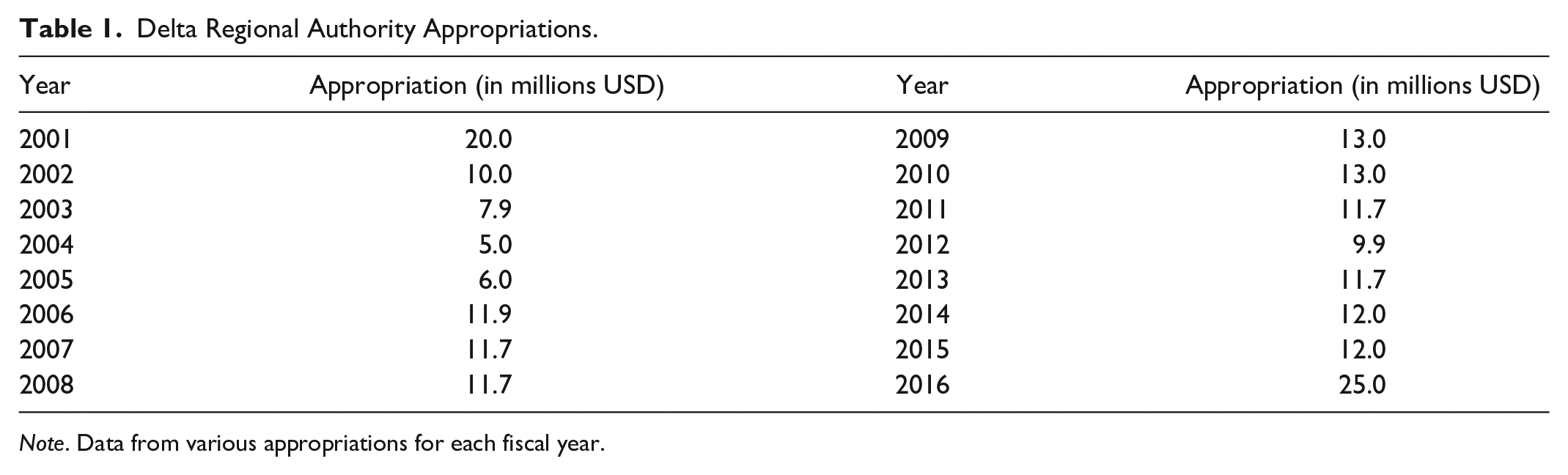
Note. Data from various appropriations for each fiscal year.

One of its more prominent projects is expanding access to quality health care. The DRA’s Delta Doctors program allows foreign physicians who trained in the United States to work in medically underserved areas of the DRA through a J-1 visa waiver. This creates an opportunity for these doctors to work in these remote areas while serving DRA constituents who have little to no access to primary or emergency health care. Another DRA initiative is the Community Health Systems Development Program, a collaboration with Health Resources and Human Services and the U.S. Department of Health and Human Services. This program attempts to improve the infrastructure of the local hospitals, clinics, and other health care organizations through a technical assistance program. This includes implementing improvements to financial operations and telehealth operations and providing social services to address challenges faced by patients like childcare and housing.

One of the DRA’s key objectives is improving the local workforce through job training programs across the region. The Re-Imagining Workforce Development program is geographically targeted to aid communities within the DRA through planning and building regional development workforce systems based on the unique characteristics of the DRA economy and structural institutions. State-run summits strive to bring together leadership, businesses, and educators to best address the changing needs of the economy and to fill the gaps in the training. In addition, the DRA runs the Delta Entrepreneurship Network to bring together small business owners to discuss, inform, and provide access to the resources needed to make small businesses thrive and to encourage their start-ups. Regarding such programs to enhance entrepreneurship, they may have especially high local economic pay-offs as found by Stephens and Partridge (2011) and Stephens et al. (2013). The DRA hopes that helping those within the region can achieve similar pay-offs.

Through the Delta Leadership Institute, the DRA links community and government leaders to address the area’s most dire issues. In bringing stakeholders together, the DRA can improve collaboration. The Delta Leadership Institute’s Executive Academy provides training, information, and networking to facilitate bringing larger groups together to address broader issues. Indeed, regional organizations such as the DRA can play a larger role as a broker that brings together the relevant players in one room. This garners a critical mass to address larger regional issues that one entity could not address alone. Similarly, the DRA can provide capacity to help identify funding sources and grant writing as well as providing small matching funding to help achieve cost-sharing thresholds for grant applications.

Another set of programs come in the form of direct funding. In its Regional Development Plan III, the DRA defined three project goals eligible for their direct funding: “advance the productivity and economic competitiveness of the Delta workforce; strengthen the Delta’s physical, digital, and capital connections to the global economy; and facilitate local capacity building within Delta communities, organizations, businesses, and individuals” (Masingill, 2016b, p. 13). The funding normally comes in the form of grants to any initiative that attempts to address one of these goals and the DRA can occasionally be the funding source as a last resort.

Method

Instrumental Variable (Two-Stage Least Squares)

The DRA’s geography, unfortunately, creates a selectivity issue for studying its effects because its counties were not randomly assigned. Rather there was an arbitrary cutoff for the program that was decided either due to the areas being sufficiently economically distressed or more likely due to political motives. Either way, it creates a potential endogeneity problem that requires the use of an IV to address treatment selectivity. Because of the nature of the program, many of the counties could have been chosen for having low outcomes in the variables we use, and this methodology should correct for this issue.

Our instrument is an indicator variable for belonging to the lower Mississippi watershed. The watershed is a purely geographical designation defined by the U.S. Geological Society. A watershed is defined as

The divide separating one drainage basin from another and in the past has been generally used to convey this meaning . . . Drainage divide, or just divide, is used to denote the boundary between one drainage area and another. (Langbein & Iseri, 1995, p. 21)

In this case, it is the water that flows or drains into the lower Mississippi River. Figure 1 provides a visualization of the instrument. On the left is a map of the counties of the DRA (Masingill, 2016a). On the right is a map of the lower Mississippi watershed (Ierardi, 2016).

Figure 1.

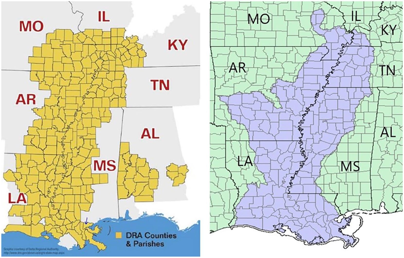
Delta Regional Authority (DRA) and watershed.

The structure of the instrument creates an issue for the DiD estimate. The DiD estimator will be biased and inconsistent if it is created using one endogenous and one exogenous variable. Falling in line with Bun and Harrison (2014), we use another instrument using the interaction of the posttreatment and watershed counties. Bun and Harrison (2014) showed that this type of interaction, under standard IV assumptions, creates a consistent and asymptotically normal estimate such that conventional IV inference can be used.

This designation should be purely exogenous to any economic variables because the watershed’s boundaries are effectively random to any individual county. They do not determine any state or county boundary and have no economic effects by themselves, or at least are conditional on the economic variables we control for, such as agricultural intensity. Yet due to the intent of the DRA, it should be highly predictive of treatment. The DRA is focused on the historically poorest counties near the lower Mississippi River Delta.

However, the instrument may have concerns relating to how well it meets the exclusion restriction. The lower Mississippi watershed may have unique factors that will affect its economic outcomes. These can include soil quality, climate, and so on. While we do not directly control for these factors, the propensity score matched counties should still have similar characteristics. By choosing counties that control demographic, economic, and employment characteristics, it should control for any of these factors. Since both the matched and treated counties have similar characteristics, the watershed should not have unique benefits, meaning the instruments meet the exclusion restriction. As noted above, our restriction should be exogenous, conditional on controlling for many of the variables that are features of the Delta including economic composition and demographics.

The instrument has the potential to act in one of two ways, depending on how additional selection and exclusion was done. First, if counties are added or removed due to political reasons rather than poor local economies, it is likely that the two-stage least squares (2SLS) estimates of the DRA estimates would increase if these counties have healthier economies. However, if additional non-Delta counties were added based on need, using IV would decrease the point DRA estimated effects because these “weaker” counties would bring down the average DRA effect.

Propensity Score Matching

In policy evaluation, a key challenge is finding a proper counterfactual. Rarely are government programs implemented using random selection with treated and control groups (i.e., Progresa in Mexico; Behrman & Hoddinott, 2005; Schultz, 2004), forcing researchers to create their own counterfactual. For example, in Ham et al. (2011), they used nearby census tracts when looking at the effect of federal Empowerment Zones. This creates a problem of possible spillovers biasing the results. Other common methodologies include propensity score matching (Rosenbaum & Rubin, 1983) and synthetic controls (Abadie & Gardeazabal, 2003; Abadie et al., 2010).

The concept of propensity scores has been in existence for decades (Hirano et al., 2003; Rosenbaum & Rubin, 1983, 1984). The idea is to find untreated regions that closely match the observational characteristics of the treated regions. This allows for the observation of regions that were similar prior to treatment to help form a credible counterfactual.

Program evaluation of this type used in this study was pioneered by Isserman and Rephann’s (1995) evaluation of the ARC. They used a similar methodology called Mahalanobis Matching by considering counties that had similar demographics and economic characteristics to those included in the ARC. They then used mean testing to see how the ARC counties performed relative to their “twins.”

In this article, we use a one-to-one propensity score matching with replacement to find counterfactual counties for those not included in the DRA. Weighting the matches on their frequency should mitigate any biases the smaller sample size may present. The matching algorithm is provided by the “PSMATCH2” user code for Stata (Leuven & Sianesi, 2001) by using a standard binary probit model to generate estimated propensity scores. Many of the control variables are similar to those in Isserman and Rephann (1995). The variables chosen are a set of many of the same economic and demographic characteristics found in their article, but in some cases more detailed. This allows us to find accurate matches for economic and population trends pretreatment. For a full list of the variables, see Table 2.

Table 2.

Propensity Score Variables.

Variable	Years	Variable	Years
Economic variables
% in poverty	1997-2001	% of children in poverty	1997-2001
% Working for federal government	1997-2001	% Working for state government	1997-2001
% Working for local government	1997-2001	% Working in goods producing	1997-2001
% Working in manufacturing	1997-2001	% Working in natural resources and mining	1997-2001
% Working in construction	1997-2001	% Working in service-providing	1997-2001
% Working in trade, transportation, and utilities	1997-2001	% Working in information	1997-2001
% Working in professional and business services	1997-2001	% Working in education and health services	1997-2001
% Working in leisure and hospitality	1997-2001	% Working in other	1997-2001
Wage growth	1996-2001	% Working in unclassified	1997-2001
ln(median income)	1997-2001	Educational attainment	2000
Demographic variables
% Male and White	1997-2001	% Female and White	1997-2001
% Male and Black	1997-2001	% Female and Black	1997-2001
% Male and Asian and Pacific Islander	1997-2001	% Female and Asian and Pacific Islander	1997-2001
% Male and Native American	1997-2001	% Female and Native American	1997-2001
Population growth	1996-2001	Rural–urban continuum codes	2003
% Net migration	2000-2001

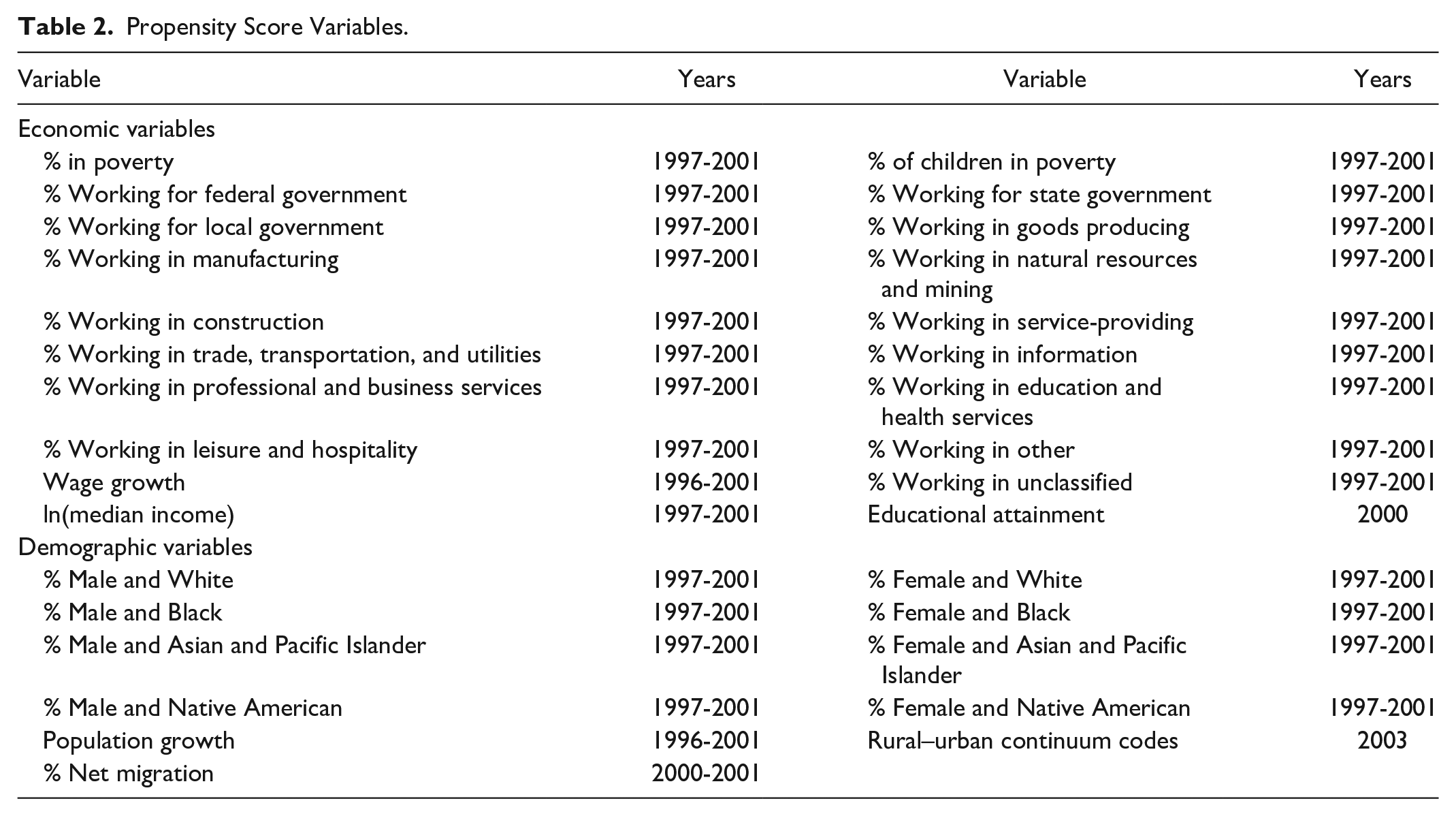
We also employ five pretreatment years to better establish pretreatment trends, rather than 1 year of pretreatment data, to help the matching algorithm find a better match. For instance, Pender and Reeder (2011) used data from 2000 as the basis for their propensity score that may be insufficient to guarantee a parallel trend for their DiD estimator. Supplemental Appendix 1 online provides graphic evidence regarding parallel trends for key economic indicators used in this study.

Econometric Structure

Our base model is the DiD estimation that is commonly used in policy evaluation (Baum-Snow & Ferreira, 2014). This methodology is chosen to give us comparison control and treatment groups. Because of the time period studied, 1997 to 2016, a simple before and after study would not suffice. Economic shocks like the Great Recession would make it hard to evaluate the effectiveness of the program. As a result, DiD gives us a comparison of untreated counties to truly see how effective the DRA was at achieving its goals compared with if it had received no treatment under the same conditions.

The model used appears as follows:

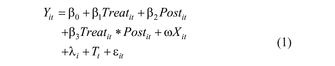
\begin{matrix} Y_{i t} = β_{0} + β_{1} T r e a t_{i t} + β_{2} P o s t_{i t} \\ + β_{3} T r e a t_{i t} * P o s t_{i t} + ω X_{i t} \\ + λ_{i} + T_{t} + ε_{i t} \end{matrix}

(1)

where Y_it represents outcome variables for count i in year t. The main outcomes we consider are median household income and poverty rates. Treat_it is an indicator variable for whether county i is included in the DRA. The comparison group for treatment will be the matched counties. Post_it represents the years starting with when the DRA became operational in 2002. Although the DRA was passed into law in 2000 (Masingill, 2016a), the tangible impacts should come from funding. Given that funding levels were relatively small, we doubt there were any measurable anticipation effects; nevertheless, we will test earlier years for the Post_it year in robustness checks. β₃ is the DiD coefficient. X_it is a matrix of control covariates. λ_i are state fixed effects. τ_t are year fixed effects.

We will also employ IV estimation to account for selectivity endogeneity. As noted above, our instrument is an indicator for whether the county is in the lower Mississippi watershed. The two first-stage equations are as follows:

T r e a t_{i} = α_{0} + α_{1} W a t e r s h e d_{i} + α_{2} X_{i t} + λ_{i} + τ_{t} + μ_{i t}

(2)

\begin{matrix} T r e a t_{i} * P o s t_{i t} = γ_{0} + γ_{1} W a t e r s h e d_{i} + γ_{2} P o s t_{i t} \\ + γ_{3} W a t e r s h e d_{i} * P o s t_{i t} + γ_{4} X_{i t} \\ + λ_{i} + τ_{t} + ν_{i t} \end{matrix}

(3)

The results of the first-stage equations are reported in Table 1. Equation 2 describes the first-stage equation for the Treat variable using Watershed as the instrument and the other control variables defined above. Equation 3 follows the structure recommended by Bun and Harrison (2014) for the Treat_i*Post_it variable using as instruments (Watershed_i), the exogenous variable (Post_it), the interaction of Watershed_i and Post_it, and the control variables.

Data

The base data are a 1997 to 2016 panal data set of U.S. counties. The demographic data are from different census databases. Median household income and poverty estimates are from the Census Small Area Income and Poverty Estimates database.² Population, net migration, and county demographics are from the Census County Population by Characteristics database. Net migration data are only available beginning in 2000 instead of 1997. Additionally, nonemployer statistics are gathered from annual estimates provided by the U.S. Census Bureau.

Information on employment, wages, and unemployment are from the Bureau of Labor Statistics. Employment and wages by industry and wages are from the Quarterly Census of Employment and Wages. The county unemployment rates are from the monthly Local Area Unemployment estimates averaged over the entire year.

Geographic information is from several different sources. The DRA counties are from the DRA Year in Review (Masingill, 2016a) and ARC counties are added from its website (Counties in Appalachia, n.d.). The TVA, unlike the ARC and DRA, does not have to cover entire counties. As a result, the data for the counties are taken from Kline and Moretti (2014). Shapefiles for the lower Mississippi watershed are provided by the U.S. Geological Survey (Ierardi, 2016).

The watershed instrument was generated by overlaying county shapefiles on the watershed shapefile in ArcGIS. The counties were defined as being in the watershed if any part of the county was in the watershed. Therefore, if no part of the county is in the watershed, it is counted as being outside the watershed.

We omit some counties from the analysis. First, counties from Alaska and Hawaii are dropped due to their extreme remoteness. Next, independent cities are omitted because there are no independent cities within the DRA. Independent cities are a small, urbanized geographic area; it is extremely unlikely that they would be a good match for rural Mississippi Delta counties. Seven parishes from Louisiana are omitted because monthly measurements were not collected from September 2005 to June 2006 due to Hurricane Katrina, making it impossible to create annual averages for those 2 years. We further omit all ARC counties because, while the ARC counties might have many observable similarities to DRA counties, the ARC is considerably better funded and has been in existence for nearly 40 years longer than the DRA. ARC counties were included in robustness checks. Finally, the counties that are part of both the ARC and the DRA have been dropped.

Table 3 shows the summary statistics for pretreatment data between the different groups in this study. The first group is the “treated” DRA counties containing all DRA counties except those that were omitted, as previously discussed. The propensity score matched counties appear to create a reasonable counterfactual. Table 3 shows that the DRA had a (nominal) average median household income of $27,757 in 2000, while the rest of the country’s average median household income was considerably higher at $35,824, or 29.1% above the DRA. Similar gaps are seen across all measures and the differences are statistically significant. However, the matched counties are fairly close in income, poverty, and unemployment measures in terms of the matched counties, and are not statistically different from the DRA counties. This illustrates that the matched counties are a much better counterfactual than the rest of the United States. Supplemental Appendix 1 shows the pre- and posttreatment trends for the dependent variables and illustrates that the treatment and control counties have parallel trends.

Table 3.

Summary Statistics Before Treatment.

	DRA counties	PSM counties	Other U.S. counties	Difference in levels	Difference in growth rate
Median HH income	27757.3 (5216.5)	29286.7 (4928.7)	35824.7 (8784.6)	***
% in poverty	0.198 (0.0587)	0.181 (0.0694)	0.132 (0.0559)	***
% children in poverty	0.254 (0.0722)	0.235 (0.0854)	0.171 (0.0781)	***
Unemployment rate	0.0684 (0.0249)	0.0686 (0.0450)	0.0467 (0.0239)	***
Nonemployer	1735.2 (3525.095)	2025.461 (2206.594)	5807.16 (20289.1)
% net migration	−0.00325 (0.00835)	−0.000275 (0.00733)	−0.000565 (0.0114)	***	***
Number of counties	236	33	2407

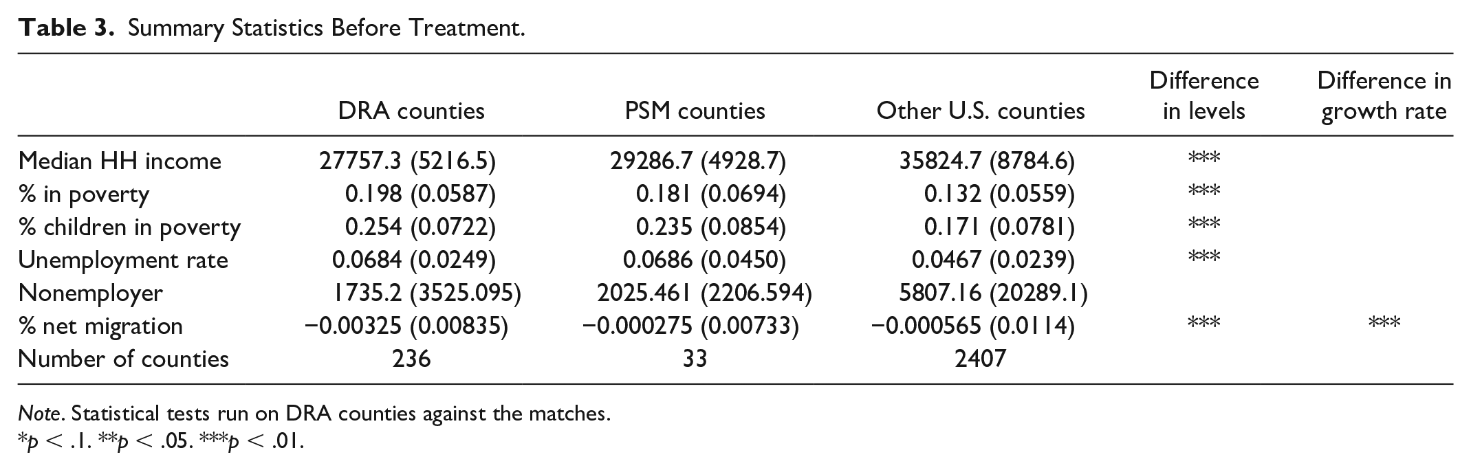
Note. Statistical tests run on DRA counties against the matches.

p < .1. **p < .05. ***p < .01.

Results

Turning to the regression results, we first discuss the first-stage results and then the second-stage IV results. For the second-stage results, the tables follow the same pattern of the first four columns, which report the ordinary least squares (OLS) estimates followed by the 2SLS estimates in Columns 5 to 8 with changes in the controls and fixed effects. Overall, we find consistent, positive economic benefits from the DRA in many of the outcome variables.

First-Stage Results

Table 4 reports the first-stage results for the two different specifications of the instrument. Recall that Watershed is a dummy variable that denotes whether a county is within the lower Mississippi watershed. Post is a dummy if the year of the panel is before or after the DRA begins its funding programs, which is 2002 or thereafter. Watershed * Post is the interaction following Bun and Harrison’s (2014) correction. Treat is a dummy for any DRA county. Column 1 depicts the first stage for just the treatment, in which the F-statistic value for the strength of the instrument is 144. Column 2 reports the first-stage results for the interaction instrument. In this case, the F-statistic regarding the strength of the instrument equals 206. In both cases, the first-stage results indicate a strong instrument for the second stage.

Table 4.

First Stage Results.

	(1) Treat	(2)Treat * post
Watershed	0.409***(0.0106)	0.108*** (0.0161)
Post		0.292***(0.0155)
Watershed * post		0.294*** (0.0182)

Observations	9,440	9,440
R ²	0.392	0.491
F	144.2	206.1

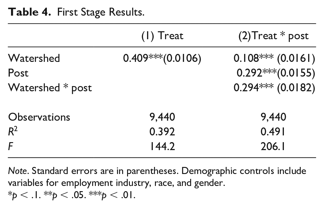
Note. Standard errors are in parentheses. Demographic controls include variables for employment industry, race, and gender.

p < .1. **p < .05. ***p < .01.

Assuming our exclusion restriction that is conditional on our control variables, contemporary economic outcome variables are not affected by being in the watershed (the exclusion restriction). The instrument is removing the political selectivity for how the boundaries of the DRA were selected.

Income

We first consider average county median household income as a welfare measure of the middle class by providing multiple OLS and 2SLS models to show robustness. Looking at Table 5, our preferred results are in columns 3 and 7 that include both year and state fixed effects and columns 4 and 8 that replace state fixed effects with county fixed effects. The trade-offs are that the county fixed-effect models are economically “stronger” as they remove county-specific, time-invariant omitted effects, not just state-omitted effects. However, this comes at the costs of removing all persistent cross-sectional effects, including those of the DRA, because such effects are picked up by the county fixed effects. This would suggest that the models with the state fixed effects may be more valid as they maintain these cross-sectional effects.

Table 5.

Median Household Income.

	OLS				2SLS
	(1)	(2)	(3)	(4)	(5)	(6)	(7)	(8)
Treatment	−0.0531*** (0.00500)	−0.0344*** (0.00397)	−0.0367*** (0.00397)		0.0645*** (0.0270)	0.0420* (0.0227)	0.0304 (0.0193)	0.418*** (0.0247)
Post 2002	0.106*** (0.00450)	0.380*** (0.00712)	0.383*** (0.00697)	0.375*** (0.00418)	0.137*** (0.0162)	0.377*** (0.0161)	0.374*** (0.0144)	0.370*** (0.00600)
Treat * post	0.0308*** (0.00566)	0.0228*** (0.00448)	0.0258*** (0.00430)	0.00923*** (0.00190)	−0.0195 (0.0315)	0.0650** (0.0263)	0.0818*** (0.0229)	0.0170** (0.00720)

Observations	9,440	9,440	9,440	9,440	9,440	9,440	9,440	9,440
R ²	0.656	0.785	0.805	0.919	0.621	0.726	0.759	0.967
Demographic controls	Yes	Yes	Yes	Yes	Yes	Yes	Yes	Yes
Year fixed effects	No	Yes	Yes	Yes	No	Yes	Yes	Yes
State fixed effects	No	No	Yes	No	No		Yes
County fixed effects	No	No	No	Yes	No	No	No	Yes

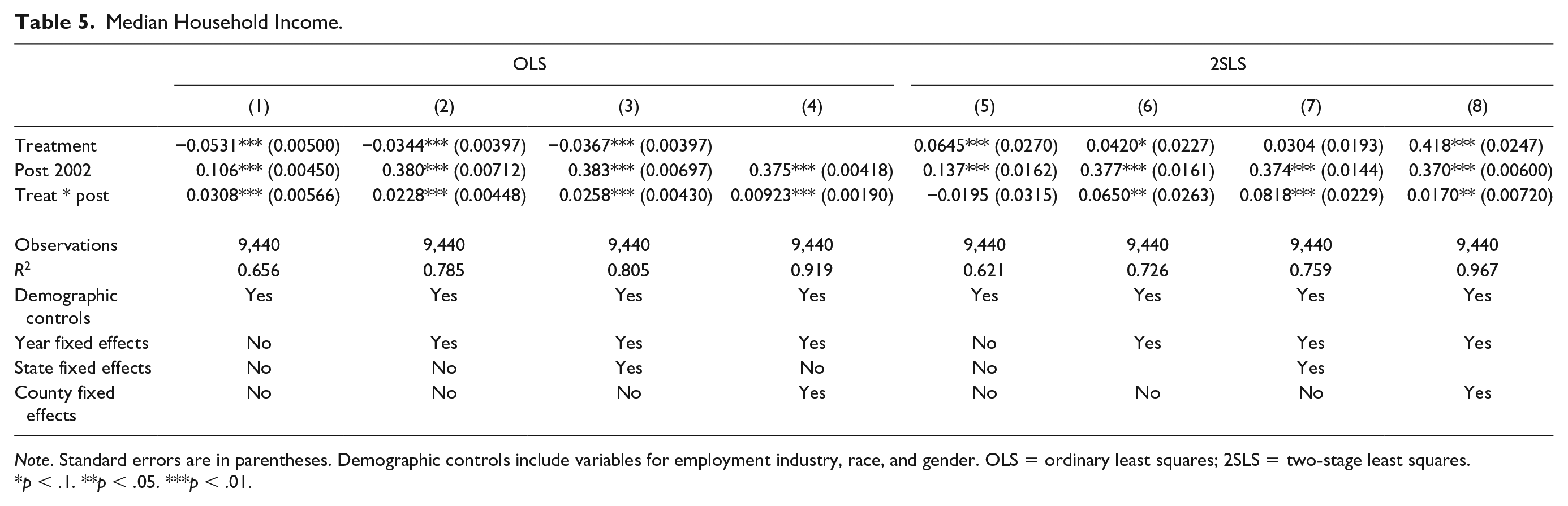
Note. Standard errors are in parentheses. Demographic controls include variables for employment industry, race, and gender. OLS = ordinary least squares; 2SLS = two-stage least squares.

p < .1. **p < .05. ***p < .01.

Using the natural log of the county’s median household income as the dependent variable, Table 5 presents the regression results. With only demographic controls in Column 1, the OLS regression results suggest that DRA counties are negatively selected with approximately 5.31% lower average median household income prior to the DRA’s operation than the matched results (or 0.0531 log points). Regarding the DRA’s influence, the results indicate that the average treatment effect of the DRA on average county median household income is approximately a statistically significant 3.08% increase. Column 2 adds year fixed effects, which reduces the DRA’s influence to approximately 2.28%. After including state and year fixed effects in Column 3, the DRA’s average treatment effect increases to approximately 2.58% compared with matched counties. For comparison, using the mean values from Table 3, the estimated positive effects equal $716 in 2000 dollars or $1,051.38 in 2018 dollars after adjusting by the Consumer Price Index. Given that the average DRA household is about 2.6 people per household, the average benefit per person is $275.38 and $404.38 (assuming the average household is approximately the same size as the median household). The DRA has spent about $13.90 per person in direct spending over the program’s lifetime, or $350 per person when including leveraged money. This would suggest that DRA expenditures have substantial returns.

The 2SLS estimates likely provide the better estimates given the endogenous selection. Jumping to Column 7 when state and year fixed effects are included, the estimated DRA treatment is now considerably larger (8.18%) and statistically significant. Even when controlling for county fixed effects in Column 8, there is still a positive and statistically significant treatment effect of 1.70%. What this further indicates is that the DRA negatively selected counties in that they were more slowly growing than one would otherwise expect.

Poverty

Poverty is clearly one of biggest challenges facing DRA counties. Despite strong national economic growth during the latter half of the 1990s for most of the country, the DRA region’s total poverty rate was about 50% greater than the national average. In addition, the DRA child poverty rate was also considerably higher (25.4% compared with 17.1%).

Keeping with the structure of Table 5, Table 6 reports the DiD results for the total poverty rate. With only demographic controls in Column 1, the OLS results suggest that the DRA is associated with a statistically significant decrease in the poverty rate of 0.653 percentage points, which seems to be similar to the results in Column 2 when adding the year fixed effects. When controlling for year and state fixed effects, the poverty-reducing effect rises to 0.734 percentage points. As before, the 2SLS results suggest that the DRA is negatively selected with larger poverty rate reductions than the corresponding OLS results (Columns 1 to 3 vs. Columns 5 to 7). Focusing on when state and year fixed effects are included (Column 7), the 2SLS show that the DRA was associated with a statistically significant 1.2 percentage point lower poverty rate (though at the 10% level). The effect changes to an increase in poverty when controlling for county fixed effects. This result potentially goes against our findings in the previous section that found positive gains in household income. Though the effect is statistically significant, it is likely due to the decreased variation from removing all persistent cross-sectional effects.

Table 6.

Percentage of People in Poverty.

	OLS				2SLS
	(1)	(2)	(3)	(4)	(5)	(6)	(7)	(8)
Treatment	0.00852*** (0.00137)	0.00933*** (0.00129)	0.00920*** (0.00126)		0.00704 (0.00719)	0.0105 (0.00662)	−0.00248 (0.00563)	−0.250*** (0.0113)
Post 2002	0.0110*** (0.00123)	0.00104 (0.00231)	0.00387* (0.00221)	0.0193*** (0.00185)	0.0174*** (0.00431)	0.00686 (0.00468)	0.00338 (0.00419)	0.00588** (0.00275)
Treat * post	−0.00653*** (0.00155)	−0.00610*** (0.00145)	−0.00734*** (0.00136)	−0.00414*** (0.000840)	−0.0214** (0.00837)	−0.0206*** (0.00766)	−0.0120* (0.00667)	0.0175*** (0.00330)

Observations	9,440	9,440	9,440	9,440	9,440	9,440	9,440	9,440
R ²	0.654	0.691	0.735	0.630	0.654	0.690	0.732	0.928
Demographic controls	Yes	Yes	Yes	Yes	Yes	Yes	Yes	Yes
Year fixed effects	No	Yes	Yes	Yes	No	Yes	Yes	Yes
State fixed effects	No	No	Yes	No	No	No	Yes	No
County fixed effects	No	No	No	Yes	No	No	No	Yes

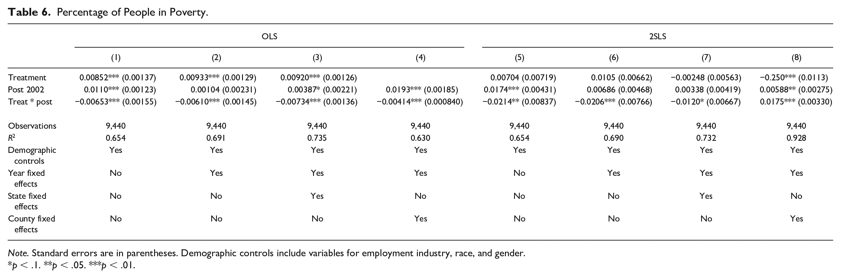
Note. Standard errors are in parentheses. Demographic controls include variables for employment industry, race, and gender.

p < .1. **p < .05. ***p < .01.

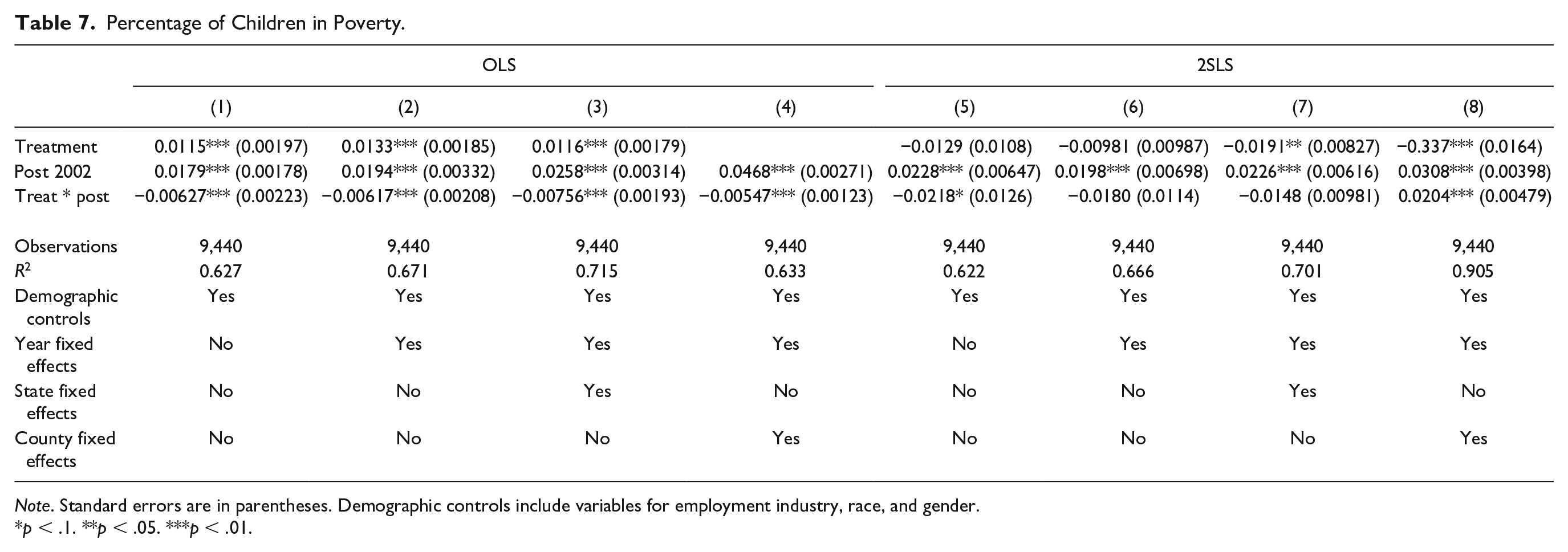
Table 7 shows the results for the child poverty rate. When including all controls in Column 3, there again seems to be a small significant decrease in child poverty. The point estimate is about −0.76 percentage points that is statistically significant. The 2SLS estimates again suggest that the DRA counties are negatively selected with relative stable point estimates that are negative and greater in magnitude than the OLS. However, only the results without year and state fixed effects (Column 5) and with year and county fixed effects (Column 8) are statistically significant. These estimates show the DRA program is associated with about 2 percentage points lower for county child poverty rates.

Table 7.

Percentage of Children in Poverty.

	OLS				2SLS
	(1)	(2)	(3)	(4)	(5)	(6)	(7)	(8)
Treatment	0.0115*** (0.00197)	0.0133*** (0.00185)	0.0116*** (0.00179)		−0.0129 (0.0108)	−0.00981 (0.00987)	−0.0191** (0.00827)	−0.337*** (0.0164)
Post 2002	0.0179*** (0.00178)	0.0194*** (0.00332)	0.0258*** (0.00314)	0.0468*** (0.00271)	0.0228*** (0.00647)	0.0198*** (0.00698)	0.0226*** (0.00616)	0.0308*** (0.00398)
Treat * post	−0.00627*** (0.00223)	−0.00617*** (0.00208)	−0.00756*** (0.00193)	−0.00547*** (0.00123)	−0.0218* (0.0126)	−0.0180 (0.0114)	−0.0148 (0.00981)	0.0204*** (0.00479)

Observations	9,440	9,440	9,440	9,440	9,440	9,440	9,440	9,440
R ²	0.627	0.671	0.715	0.633	0.622	0.666	0.701	0.905
Demographic controls	Yes	Yes	Yes	Yes	Yes	Yes	Yes	Yes
Year fixed effects	No	Yes	Yes	Yes	No	Yes	Yes	Yes
State fixed effects	No	No	Yes	No	No	No	Yes	No
County fixed effects	No	No	No	Yes	No	No	No	Yes

Note. Standard errors are in parentheses. Demographic controls include variables for employment industry, race, and gender.

p < .1. **p < .05. ***p < .01.

These results show that the DRA has mixed impacts on total and child poverty, though most of the estimates suggest that it has a negative effect. It should be noted that the results are not as precisely estimated as the median household income results but, in general, suggest positive effects for the DRA.

Unemployment

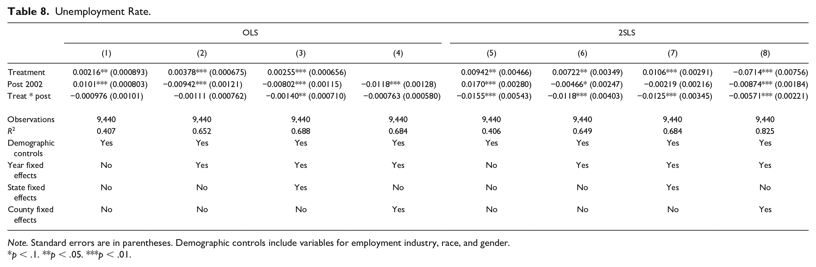
One of the important goals of the DRA was to promote employment opportunities. To appraise this, we first consider county unemployment rates. Pretreatment, the average 2000 DRA county unemployment rate was 46.5% higher compared with the rest of the country, or the corresponding 2000 unemployment rate levels were 6.84% in the DRA compared with 4.67% in the rest of the country.

The unemployment rate results are shown in Table 8. Unemployment rates appear to decline more in the treated DRA counties relative to their matched counties, though again in the OLS estimates the results are not precisely estimated. With the state and year fixed effects (Column 3), the DRA is associated with about a statistically significant 0.14 percentage point lower unemployment rate. The 2SLS estimates continue to tell a negative selectivity story with negative estimates in the negative 1 percentage point range. When examining the model with state and year fixed effects (Column 7), the unemployment rate in the DRA counties appears to be about 1.25 percentage points lower compared with the matched counties. The effect with county and year fixed effects (Column 8) shows similar results, though the magnitude of the effect is reduced by about half.

Table 8.

Unemployment Rate.

	OLS				2SLS
	(1)	(2)	(3)	(4)	(5)	(6)	(7)	(8)
Treatment	0.00216** (0.000893)	0.00378*** (0.000675)	0.00255*** (0.000656)		0.00942** (0.00466)	0.00722** (0.00349)	0.0106*** (0.00291)	−0.0714*** (0.00756)
Post 2002	0.0101*** (0.000803)	−0.00942*** (0.00121)	−0.00802*** (0.00115)	−0.0118*** (0.00128)	0.0170*** (0.00280)	−0.00466* (0.00247)	−0.00219 (0.00216)	−0.00874*** (0.00184)
Treat * post	−0.000976 (0.00101)	−0.00111 (0.000762)	−0.00140** (0.000710)	−0.000763 (0.000580)	−0.0155*** (0.00543)	−0.0118*** (0.00403)	−0.0125*** (0.00345)	−0.00571*** (0.00221)

Observations	9,440	9,440	9,440	9,440	9,440	9,440	9,440	9,440
R ²	0.407	0.652	0.688	0.684	0.406	0.649	0.684	0.825
Demographic controls	Yes	Yes	Yes	Yes	Yes	Yes	Yes	Yes
Year fixed effects	No	Yes	Yes	Yes	No	Yes	Yes	Yes
State fixed effects	No	No	Yes	No	No	No	Yes	No
County fixed effects	No	No	No	Yes	No	No	No	Yes

Note. Standard errors are in parentheses. Demographic controls include variables for employment industry, race, and gender.

p < .1. **p < .05. ***p < .01.

The decrease in the unemployment rate falls in line with many of the assertions made by the DRA. The DRA has claimed, over its existence, that it has helped create or retain 26,218 jobs (Masingill, 2016a). While self-reported evaluations should always be treated skeptically, the evidence is consistent with the DRA improving the local labor market. Consequently, if at least the direction of the DRA’s self-reported estimate is accurate, this change in unemployment is expected.

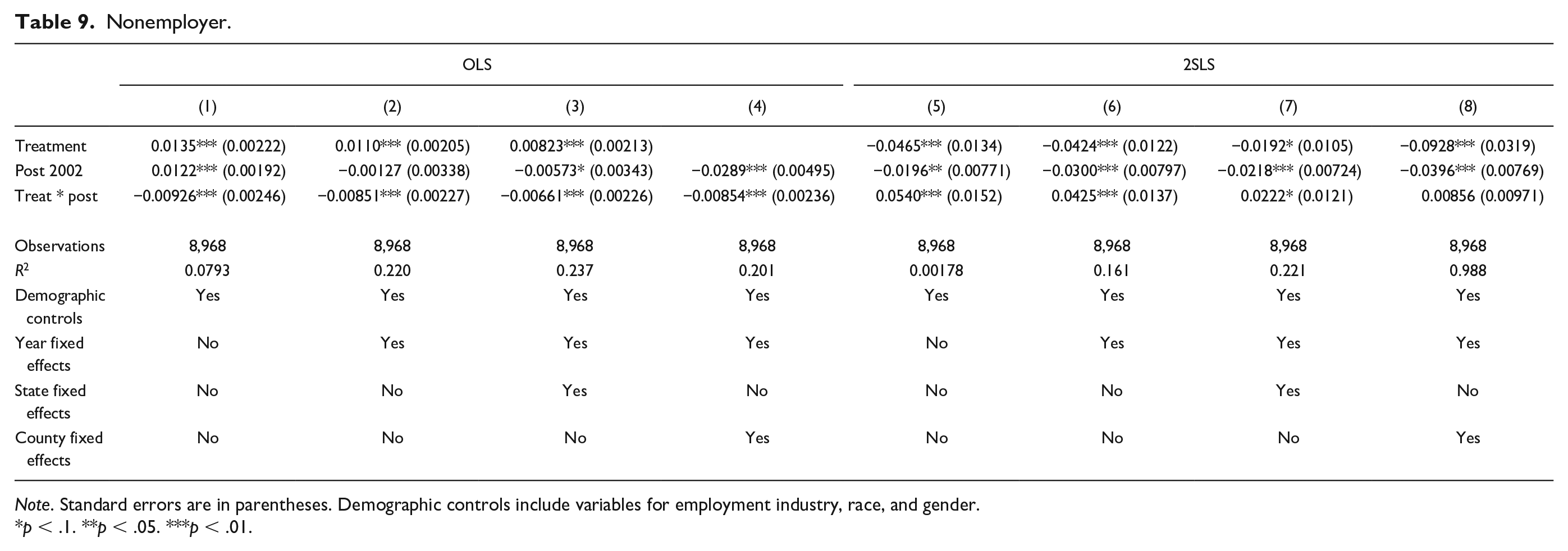
Self-Employment

One of the largest programs the DRA provides is to promote and develop entrepreneurship (Masingill, 2016a). To explore this, we use rate of change of the Census Bureau’s Nonemployer Statistics.³ While this is only a proxy for entrepreneurship, it covers most of the self-employment and new businesses in the region, which is a worthy goal in itself. There is also a substantial amount of evidence supporting the benefits self-employment can have (i.e., Rupasingha & Goetz, 2013). The regression results are reported in Table 9.

Table 9.

Nonemployer.

	OLS				2SLS
	(1)	(2)	(3)	(4)	(5)	(6)	(7)	(8)
Treatment	0.0135*** (0.00222)	0.0110*** (0.00205)	0.00823*** (0.00213)		−0.0465*** (0.0134)	−0.0424*** (0.0122)	−0.0192* (0.0105)	−0.0928*** (0.0319)
Post 2002	0.0122*** (0.00192)	−0.00127 (0.00338)	−0.00573* (0.00343)	−0.0289*** (0.00495)	−0.0196** (0.00771)	−0.0300*** (0.00797)	−0.0218*** (0.00724)	−0.0396*** (0.00769)
Treat * post	−0.00926*** (0.00246)	−0.00851*** (0.00227)	−0.00661*** (0.00226)	−0.00854*** (0.00236)	0.0540*** (0.0152)	0.0425*** (0.0137)	0.0222* (0.0121)	0.00856 (0.00971)

Observations	8,968	8,968	8,968	8,968	8,968	8,968	8,968	8,968
R ²	0.0793	0.220	0.237	0.201	0.00178	0.161	0.221	0.988
Demographic controls	Yes	Yes	Yes	Yes	Yes	Yes	Yes	Yes
Year fixed effects	No	Yes	Yes	Yes	No	Yes	Yes	Yes
State fixed effects	No	No	Yes	No	No	No	Yes	No
County fixed effects	No	No	No	Yes	No	No	No	Yes

Note. Standard errors are in parentheses. Demographic controls include variables for employment industry, race, and gender.

p < .1. **p < .05. ***p < .01.

In the OLS model, the point estimates are slightly negative and statistically significant. However, the 2SLS results show the positive and significant results, suggesting favorable DRA effects. In Column 7, for instance, there is a 2.22 percentage point increase in the number of new nonemployers being formed over the matched counties. All the 2SLS results show similar point estimates, with the exception of those in Column 8. This is quite notable given the national rate of nonemployer increase over the same time period averaged 1.55%. These results suggest that the DRA is meeting its entrepreneurship goals. The counties are experiencing a boom in new small firms over their matched counties, consistent with success in the Delta Entrepreneurship Network.

Net Migration

The previous results generally show positive economic effects. There are positive gains in income, decreases in unemployment and poverty, and generally positive effects on business start-ups. One possible reason for this is an influx of migrants, especially high-skill migrants. For example, programs like Delta Doctors aim to attract high-skill health care workers into the DRA to address current shortages. Likewise, we may expect inward net migration if the DRA generally increases employment opportunities.

Table 10 reports corresponding results using annual net migration as a percentage of total county population from 2000 to 2015 as the dependent variable. Results from Table 10 suggest weak negative effects from the DRA’s efforts. That is, the point estimates are negative, but only in the OLS models with state and year fixed effects (Column 3) and the IV results with county fixed effects (Column 8) are statistically significant. Overall, it is only possible to say that the DRA was not increasing net migration (though it may have been negative), which may be desired to ensure that the original low-income residents are the ones benefiting from DRA policy. A typical positive criterion of place-based policy is imperfect labor force mobility (Bartik, 1991; Partridge et al., 2015a; 2015b). To be sure, it is still possible that high-skilled migrants are in-migrating, but this is overwhelmed by net migration of low-skilled workers.

Table 10.

Net Migration.

	OLS				2SLS
	(1)	(2)	(3)	(4)	(5)	(6)	(7)	(8)
Treatment	0.000106 (0.000303)	0.000330 (0.000279)	0.000309 (0.000282)		−0.0000806 (0.00277)	−0.00105 (0.00248)	−0.000772 (0.00213)	0.0322*** (0.00415)
Post 2002	0.0000902 (0.000237)	0.00371*** (0.000346)	0.00357*** (0.000349)	0.00322*** (0.000446)	0.000867 (0.00146)	0.00360*** (0.00134)	0.00362*** (0.00120)	0.00483*** (0.00101)
Treat * post	−0.000271 (0.000320)	−0.000396 (0.000293)	−0.000533* (0.000290)	−0.000307 (0.000271)	−0.00202 (0.00297)	−0.000538 (0.00266)	−0.00114 (0.00231)	−0.00301* (0.00156)

Observations	8,024	8,024	8,024	8,024	8,024	8,024	8,024	8,024
R ²	0.824	0.833	0.843	0.819	0.824	0.833	0.843	0.797
Demographic controls	Yes	Yes	Yes	Yes	Yes	Yes	Yes	Yes
Year fixed effects	No	Yes	Yes	Yes	No	Yes	Yes	Yes
State fixed effects	No	No	Yes	No	No	No	Yes	No
County fixed effects	No	No	No	Yes	No	No	No	Yes

Note. Standard errors are in parentheses. Demographic controls include variables for employment industry, race, and gender.

p < .1. **p < .05. ***p < .01.

DRA Dynamic Effects Over Time

A possible weakness is that the previous models assume that the DRA’s treatment effect begins immediately and remains unchanged thereafter. A more likely dynamic pattern is that the DRA’s treatment effect initially rises as it begins to operate and then levels off over time because it takes time for the DRA to affect outcomes. Thus, we explored how the DRA’s treatment effects varied over time. Our regression model is the exact same as Equations 1 to 3 from the section on poverty; however, Treatment * Post was replaced by Treatment * Year in which Year is a dummy variable for each year from 2002 onward. The IV correction is applied for each Treatment * Year variable. The results are reported in Supplemental Appendix 2 and only show one OLS and 2SLS regression with demographic controls and state and year fixed effects.

First, we consider the median income change models in Table 11 of Supplemental Appendix 2. Both OLS and IV regression results show nearly identical results in terms of magnitude and significance. In the OLS result, it takes until 2006 for positive growth to occur; however, sustained positive effects over the matched counties are not noticeable until 2009. Post 2009, there is a consistent higher level of income hovering around 3%. The 2SLS results show positive sustained growth starting in 2007 instead of 2009 with a larger magnitude (somewhere normally between 3% and 4%). These results suggest that by assuming an average treatment effect that does not vary time, our previous median household income results appear to have underestimated the contemporaneous effects of the DRA after its influence more strongly took hold.

The poverty trend results are unclear. The total poverty results from Table 12 (of Supplemental Appendix 2) show no clear or statistically significant impact. The results for child poverty are a bit more complex. The OLS results provide some evidence of a growing impact on child poverty, with a decrease of about 1.5%. The 2SLS results show no consistent change in the child poverty rate. Despite this, the point estimates are mostly negative. This would suggest there is some negative trend on poverty.

In Table 14 of Supplemental Appendix 2, the OLS unemployment results suggest the DRA’s decreasing effects do not kick in until 2006. The IV results indicate a less clear trend, though during the 2009 to 2010 period the effects are negative and statically significant. This provides evidence that during the Great Recession and its immediate aftermath, the DRA provided needed help in reducing unemployment.

Finally, both the IV and OLS net migration results continue to show no consistent DRA pattern over time.

Robustness Checks

This section presents some robustness checks of the results in Conclusion section. That is, we explore the impact of other possible alternative specifications that could lead to different results. We find that the results remain generally robust to these methodological changes.

ARC Included

As noted above, we did not include the ARC counties as possible candidates in the pool of possible match counties, though this came at the cost of losing many counties that would have provided closer matches, providing a better counterfactual. They also increase the number of matched counties to 90 from 33 in the counterfactual. Generally, we would expect that if the better-funded and more-established ARC was successful in improving its counties’ outcomes, that would reduce the estimated effects of the DRA.

Perhaps surprisingly, most of the conclusions do not tangibly change. All estimates remain the same sign and generally the same statistical significance, only the point estimates slightly change; however, they continue to support a general theme that the DRA has modest positive effects.

Different Treatment Year

As described above, the DRA became law in 2000, but did not become operational until 2002. If there were any tangible anticipation effects, it would make sense to start the treatment effects in 2000. As a result, we assess the robustness of the results using 2000 as the beginning of the DRA’s treatment. Net migration results are not reported, as there would be no pretreatment years due to data availability.

There are some differences from using 2002 as treatment compared with 2000. First, median income has considerably smaller impacts. Median income goes up by about 3% compared with about 8% before. Next, unemployment rate estimates show smaller impacts, dropping by 0.612 percentage points compared with 1.25. Finally, poverty rate shows no significant impacts. One reason for the smaller results could reflect from the negative selection of the DRA counties (i.e., they were doing worse than their matched counterparts prior to the DRA).

Adjusting the Matching Algorithm

Another possible concern is our use of one-to-one matching with replacement for the propensity score matched counties. This results in only 33 counties being used when matched. To address this, we change the matching algorithm by using nearest-neighbor matching with replacement and three matches, the same algorithm used by Pender and Reeder (2011). This is a difference from one-to-one, but the algorithm finds three untreated counties that matches closest on observable characteristics instead of one. With that exception, the algorithm works the same, and each matched control country is weighted evenly in the regression. This method is common in the literature and should add more control counties against which to compare.

The results suggest that three nearest-neighbor matching seems inferior in identifying close matches to the treatment counties. Before treatment begins, the nearest-neighbor matches have higher incomes, lower poverty rates, and lower unemployment. The outcome variable means for the matched counties are farther from the DRA county means than when one-to-one matching is used. Thus, even though the nearest neighbor has a larger sample of control counties (61 compared with 33), it may come at the cost of accurate controls.

Turning to these regression results, the main results are fairly robust. For median income, the results from the three nearest-neighbor matches seem to be of slightly smaller magnitude than the base results, whereas statistical significance is also little changed. These results are consistent across the other economic measures in terms of magnitude of the coefficients and their statistical significance.

Limitations

The primary limitation of this study is that the exact beneficiary of the benefits we name cannot be identified, though there is some evidence that it seems to be around the median household. One good question in evaluating the program is are these the intended beneficiaries, or more generally who are the beneficiaries? Are these beneficiaries the local populace or new migrants to the area? This would require micro individual-level data from the American Community Survey, which would be an excellent future research step for the DRA and most other economic development programs.

Conclusion

Given the growing interest in place-based policies, this article assesses a relatively small policy intervention: the Delta Regional Authority. We ask whether small, place-based programs like the DRA have any measurable efforts and in turn, whether they are even worth the effort beyond an appearance of trying something. This article explores the economic impact of the DRA on its member counties—the first article to examine its longer-run outcomes. We use the lower Mississippi watershed as a unique IV to correct for selection bias into the DRA. Using this correction, along with propensity score matching, we assess the effectiveness of the DRA.

Using both OLS and IV DiD estimation, we find a number of significant economic benefits to the DRA. There are positive benefits to unemployment and income growth, and it appears to decrease child poverty. However, it had no measurable impact on net migration. Overall, the program increases annual median household income by $1051.38, assuming its benefits are uniform across the income distribution. Assuming the benefits for the average person are the same as the average per person in median household income, the total income gain is $4,043,769,230. Given that its budget is quite small ($138 million as of Fiscal Year 2015), the program appears to easily pass cost–benefit analysis. One possible reason for its relative success is that the relatively small nature of the DRA allows it to pick only the worthiest initiatives with the highest rate of return. While at the margin, this does suggest that expanding the DRA would be beneficial, it is not guaranteed if the program was greatly expanded whether we would continue to observe such a high pay-off. Indeed, this federal–state commission can bring all the relative federal, state, and local governments and stakeholders together to cooperate. Nonetheless, the DRA appears to be benefiting one of the poorest regions in the country at very little cost.

There is much work that can be done to further research in this field. First, using a synthetic control method has the potential to create a better counterfactual with a more varied donor pool. In this study, there were very few counties that matched to the treated counties. Using a synthetic control method, the mix of several counties would allow a researcher to exploit additional variation among the control and treated groups. We also did not consider many potential economic indicators that should be explored, including (but not limited to) health outcomes (given the DRA’s health care focus) and happiness indicators. Another example is conducting a more detailed sectoral analysis of the DRA’s effects to assess which industries are being helped or harmed by its programming. Further work could also be expanded into looking to similar programs like the Northern Great Plains Regional Authority or the Denali Commission.

Supplemental Material

EDQ-19-0086-R1-Supplemental_material – Supplemental material for The Impact of Small Regional Economic Development Commissions: Is There Any Bang After Just a Few Bucks?

Supplemental material, EDQ-19-0086-R1-Supplemental_material for The Impact of Small Regional Economic Development Commissions: Is There Any Bang After Just a Few Bucks? by Tyler Morin and Mark Partridge in Economic Development Quarterly

Footnotes

Declaration of Conflicting Interests

The author(s) declared no potential conflicts of interest with respect to the research, authorship, and/or publication of this article.

Funding

The author(s) received no financial support for the research, authorship, and/or publication of this article.

ORCID iD

Tyler Morin

Supplemental Material

Supplemental material for this article is available online.

Notes

Author Biographies

Tyler Morin is a fifth-year PhD candidate at The Ohio State University in the AED Economics Department. He received his bachelor’s degree in economics and master’s degree in applied economics from The Ohio State University. He is interested in rural economic development and rural real estate.

Mark Partridge is the C. William Swank Chair of Rural-Urban Policy at The Ohio State University and a professor in the AED Economics Department. He is also an adjunct professor at Jinan University, Guangzhou (China) and at Gran Sasso Science Institute, L’Aquila (Italy). Professor Partridge has published in this journal as well as the American Economic Review, Journal of Economic Geography, Journal of International Economics, Journal of Urban Economics, Journal of Business and Economic Statistics, and Review of Economics and Statistics.

References

Abadie

Diamond

Hainmueller

(2010). Synthetic control methods for comparative case studies: Estimating the effect of California’s tobacco control program. Journal of the American Statistical Association, 105(490), 493-505. https://doi.org/10.1198/jasa.2009.ap08746

Abadie

Gardeazabal

(2003). The economic costs of conflict: A case-control study for the Basque Country. American Economic Review, 93(1), 113-132. https://doi.org/10.1257/000282803321455188

Austin

Glaeser

Summers

(2018). Saving the Heartland: Place-based policies in 21st century America (Working Paper 24548). https://doi.org/10.3386/w24548

Barca

McCann

Rodriguez-Pose

(2012). The case for regional development intervention: Place-based versus place-neutral approaches. Journal of Regional Science, 52(1), 134-152. https://doi.org/10.1111/j.1467-9787.2011.00756.x

Barrows

R. L.

Bromley

D. W.

(1975). Employment impacts of the Economic Development Administrations Public Works program. American Journal of Agricultural Economics, 57(1), 46-54. https://doi.org/10.2307/1238839

Bartik

T. J.

(1991). Who benefits from state and local economic development policies? W.E. Upjohn Institute for Employment Research. https://doi.org/10.17848/9780585223940

Baum-Snow

Ferreira

(2014). Causal inference in urban and regional economics (NBER Working Paper No. 20535). https://doi.org/10.3386/w20535

Behrman

J. R.

Hoddinott

(2005). Program evaluation with unobserved heterogeneity and selective implementation: The Mexican PROGRESA impact on child nutrition. Oxford Bulletin of Economics and Statistics, 67(4), 547-569. https://doi.org/10.1111/j.1468-0084.2005.00131.x

Brandow

Weisbrod

Collins

Howard

Bischak

(2000). Evaluation of the Appalachian Regional Commission’s infrastructure and public works program projects. Appalachian Regional Commission. https://www.arc.gov/research/researchreportdetails.asp?REPORT_ID=64

10.

Bun

M. G.

Harrison

T. D.

(2014). OLS and IV estimation of regression models including endogenous interaction terms (UVA Econometrics Discussion Paper, 2014-03). University of Amsterdam.

11.

Burchell

Dolphin

Shad

Zakrewsky

Pignataro

Griffis

Epling

Haughwout

Varady

Looye

(1997). Public works program–Performance evaluation: Final report (EDA Project No. 99-06-07415). Prepared for U.S. Department of Commerce, Economic Development Administration, Office of Program Research and Evaluation.

12.

Burchell

Haughwout

Robison

Shad

Dolphin

(1998). Public works programs–Multiplier and employment-generating effects (EDA Project No. 99-06-07415). Prepared for U.S. Department of Commerce, Economic Development Administration Office of Program Research and Evaluation.

13.

Busso

Gregory

Kline

(2013). Assessing the incidence and efficiency of a prominent place based policy. American Economic Review, 103(2), 897-947. https://doi.org/10.1257/aer.103.2.897

14.

Ciscel

D. H.

(1999). Creating economic growth in rural Mississippi Delta Counties. Federal Reserve Bank of St. Louis. https://www.stlouisfed.org/publications/bridges/fall-1999/creating-economic-growth-in-rural-mississippi-delta-counties

15.

Counties in Appalachia. (n.d.). Appalachian Regional Commission. https://www.arc.gov/appalachian_region/CountiesinAppalachia.asp#:~:text=The%20following%20independent%20cities%20in,Galax%20(Carroll%20County)%2C%20Lexington

16.

Delta Regional Authority Act, S. 1622, 106 Cong. (1999). (Enacted).

17.

Freshwater

Wojan

Goetz

(1997). Testing for the Effects of Federal Economic Development Agencies (TVA Rural Studies Staff Paper No. 97-2). University of Kentucky.

18.

Glaeser

E. L.

Gottlieb

J. D.

(2008). The economics of place-making policies. Brookings Papers on Economic Activity, 2008(1), 155-253. https://doi.org/10.1353/eca.0.0005

19.

Ham

J. C.

Swenson

İmrohoroğlu

Song

(2011). Government programs can improve local labor markets: Evidence from State Enterprise Zones, Federal Empowerment Zones and Federal Enterprise Community. Journal of Public Economics, 95(7), 779-797. https://doi.org/10.1016/j.jpubeco.2010.11.027

20.

Hirano

Imbens

Ridder

(2003). Efficient estimation of average treatment effects using the estimated propensity score. Econometrica, 71(4), 1161-1189. https://doi.org/10.1111/1468-0262.00442

21.

Ierardi

M. C.

(2016). Science in your watershed. United States Geological Society.

22.

Isserman

Rephann

T. J.

(1995). The economic effects of the Appalachian Regional Commission: An empirical assessment of 26 years of regional development planning. Journal of the American Planning Association, 61(3), 345-364. https://doi.org/10.1080/01944369508975647

23.

Kline

(2010). Place based policies, heterogeneity, and agglomeration. American Economic Review, 100(2), 383-387. https://doi.org/10.1257/aer.100.2.383

24.

Kline

Moretti

(2014). Local economic development, agglomeration economies, and the big push: 100 years of evidence from the Tennessee Valley Authority. Quarterly Journal of Economics, 129(1), 275-331. https://doi.org/10.1093/qje/qjt034

25.

Langbein

W. B.

Iseri

K. T.

(1995). General introduction and hydrologic definitions. United States Geological Society. https://doi.org/10.3133/wsp1541A

26.

Leuven

Sianesi

(2001). Mahalanobis and propensity score matching. http://repec.org/bocode/p/psmatch2.html

27.

Liebschutz

(1995). Empowerment Zones and Enterprise Communities: Reinventing federalism for distressed communities. Journal of Federalism, 25(3), 117-132. https://doi.org/10.2307/3330690

28.

Lower Mississippi Delta Development Act, S. 2246, 100 Cong. (1988).

29.

Martin

R. C.

Graham

R. E.

Jr. (1980). The impact of Economic Development Administration Programs: Some empirical evidence. Review of Economics and Statistics, 62(1), 52-62. https://doi.org/10.2307/1924272

30.

Masingill

C. A.

(2016a). Fiscal Year 2017 Budget Justification and 2015 Annual Report. Delta Regional Authority.

31.

Masingill

C. A.

(2016b). Moving the Delta forward: Delta Regional Development Plan III. Delta Regional Authority.

32.

Partridge

M. D.

(2013). America’s job crisis and the role of regional economic development policy. Review of Regional Studies, 43(2/3), 93-110.

33.

Partridge

M. D.

Rickman

D. S.

(2006). The geography of American poverty: Is there a role for place-based policies? W.E. Upjohn Institute for Employment Research.

34.

Partridge

M. D.

Rickman

D. S.

Olfert

M. R.

Tang

(2015a). U.S. regional poverty post-2000: The lost decade. Economic Development Quarterly, 29(1), 38-48. https://doi.org/10.1177/0891242414560814

35.

Partridge

M. D.

Rickman

D. S.

Olfert

M. R.

Tang

(2015b). When spatial equilibrium fails: Is place-based policy second best? Regional Studies, 49(8), 1303-1325. https://doi.org/10.1080/00343404.2013.837999

36.

Pender

Reeder

(2011). Impacts of regional approaches to rural development: Initial evidence on the Delta Regional Authority (Report No. 119). https://www.ers.usda.gov/publications/pub-details/?pubid=44857

37.

Reynolds

Rohlin

(2015, July). The effects of location-based tax policies on the distribution of household income: Evidence from the federal Empowerment Zone program. Journal of Urban Economics, 88, 1-15. https://doi.org/10.1016/j.jue.2015.04.003

38.

Rosenbaum

P. R.

Rubin

D. B.

(1983). The central role of the propensity score in observational studies for causal effects. Biometrika, 70(1), 41-55. https://doi.org/10.1093/biomet/70.1.41

39.

Rosenbaum

P. R.

Rubin

D. B.

(1984). Reducing bias in observational studies using subclassification on the propensity score. Journal of the American Statistical Association, 79(387), 516-524. https://doi.org/10.2307/2288398

40.

Rupasingha

Goetz

. (2013). Self-employment and local economic performance: Evidence from U.S. counties. Papers in Regional Science, 92(1), 141-161. https://doi.org/10.1111/j.1435-5957.2011.00396.x

41.

Schultz

T. P.

(2004). School subsidies for the poor: Evaluating the Mexican Progresa poverty program. Journal of Development Economics, 74(1), 199-250. https://doi.org/10.1016/j.jdeveco.2003.12.009

42.

Stephens

Partridge

M. D.

(2011). Do entrepreneurs enhance economic growth in lagging regions? Growth and Change, 42(1), 431-465. https://doi.org/10.1111/j.1468-2257.2011.00563.x

43.

Stephens

Partridge

M. D.

Faggian

(2013). Innovation, entrepreneurship and economic growth in lagging regions. Journal of Regional Science, 53(5), 778-812. https://doi.org/10.1111/jors.12019

Supplementary Material

Please find the following supplemental material available below.

For Open Access articles published under a Creative Commons License, all supplemental material carries the same license as the article it is associated with.

For non-Open Access articles published, all supplemental material carries a non-exclusive license, and permission requests for re-use of supplemental material or any part of supplemental material shall be sent directly to the copyright owner as specified in the copyright notice associated with the article.

0.00 MB

0.62 MB