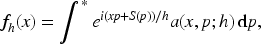
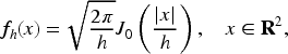
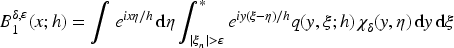
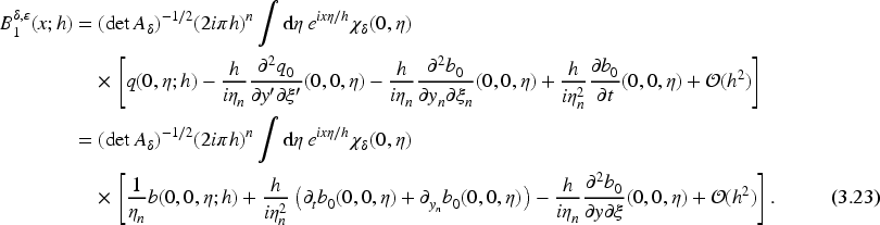
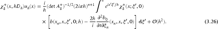
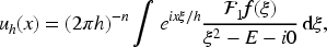
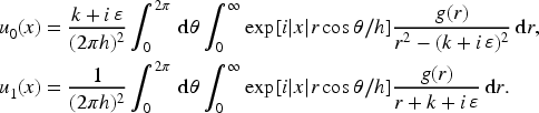
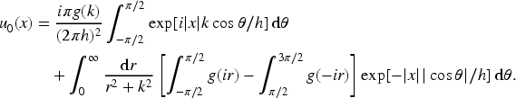
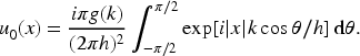
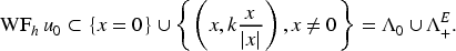
Semi-Classical Green Functions and Lagrangian Intersection. Applications to the Propagation of Bessel Beams in Non-Homogeneous Media

Abstract

We study semi-classical asymptotics for problems with localized right-hand sides by considering a Hamiltonian $H (x, p)$ positively homogeneous of degree $m \geq 1$ on $T^{*} R^{n} ∖ 0$ . The energy shell is $H (x, p) = E$ , and the right-hand side $f_{h}$ is microlocalized: (1) on the vertical plane $Λ_{0} = {x = x_{0}}$ ; (2) on the “cylinder” $Λ_{0} = {(X, P) = (φ ω (ψ), ω (ψ)); φ \in R, ω (ψ) = (\cos ψ, \sin ψ)}$ , when $n = 2$ . Most precise results are obtained in the isotropic case $H (x, p) = | p |^{m} / ρ (x)$ , with $ρ$ a smooth positive function. In case (2), $Λ_{0}$ is the frequency set of Bessel function $J_{0} (| x | / h)$ , and the solution $u_{h}$ of $(H (x, h D_{x}) - E) u_{h} = f_{h}$ when $m = 1$ , already provides an insight in the structure of “Bessel beams,” which arise in the theory of optical fibers. We present some extensions of our previous works with A. Anikin, S. Dobrokhotov and V. Nazaikinskii. In Section 3, we sketch the semi-classical counterpart of the construction of parametrices for the Cauchy problem with Lagrangian intersections, as is set up by Melrose and Uhlmann. This involves Maslov bi-canonical operator.

1. Introduction

Let $M = R^{n}$ , or possibly a smooth manifold. Write $⟨ θ ⟩ = (1 + θ^{2})^{1 / 2}$ . For $m, k \in Z$ , we recall (see e.g., Ivrii, 1998, Chapter 1) the usual class of symbols

\begin{aligned} S_{m}^{k} (M \times M \times R^{N}) = {a (x, y, θ; h) \in C^{\infty} : | \partial_{(x, y)}^{α} \partial_{θ}^{β} a (x, y, θ; h) | \leq C_{α, β} h^{k} ⟨ θ ⟩^{m - | β |}}, \end{aligned}

with asymptotic expansion

a (x, y, θ; h) \sim h^{k} (a_{0} (x, y, θ) + h a_{1} (x, y, θ) + \dots)

. We define analogously

S_{m}^{k} (T^{*} M)

. Most of the time, we shall consider symbols compactly supported in

θ

. Let

H (x, h D_{x}; h)

be a

h

-PDO whose symbol

H

belongs to

S_{m}^{0} (T^{*} M)

, or

S_{m}^{0} (T^{*} M ∖ 0)

, which is, for instance, the case when

H (x, p; h)

is positively homogeneous of degree

m

with respect to

p

. We will denote by

z = (x, p)

or by

z = (x, ξ)

a point in

T^{*} M

. Let

E \neq 0

be a non-critical energy level for Hamiltonian

H_{0}

. Let also

f_{h}

be a Lagrangian semi-classical distribution locally of the form

\begin{aligned} f_{h} (x) = (2 π h)^{- n / 2} \int_{R^{n}} e^{i φ (x, θ) / h} a (x, θ; h) d θ, \end{aligned}

(1.1)

where

φ

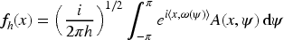
is a non-degenerate phase function in the sense of Hörmander (or a generating family in the sense of Arnold) defining the Lagrangian manifold

Λ_{0}

(see Section 3), and

a \in S_{0}^{k} (M \times R^{n})

for some

k

. We assume here

a

to be compactly supported in

θ

, excluding, for example, the case

a = 1

φ (x, θ) = ⟨ x, θ ⟩

, corresponding to

f_{h} (x) = δ (x)

, which is too singular from our point of view. For brevity we will often denote such a (normalized) integral, possibly including Maslov index factor such as

e^{i π n / 4}

, simply by

\int^{*} (\dots)

We shall assume that Hamiltonian vector field $v_{H_{0}}$ is transverse to $Λ_{0}$ , which we call Lagrangian intersection. In the articles Anikin et al. (2017, 2018, 2023), we have considered in the context of Maslov canonical operator the problem of “semi-classical Green functions,” which consists in solving $(H - E) u_{h} = f_{h}$ , $Λ_{0}$ being the vertical plane $x = x_{0}$ , with $u_{h}$ outgoing at infinity. The distributions $u_{h}$ and $f_{h}$ are linearly related by $u_{h} = E_{+} (h) f_{h}$ , where $E_{+} (h)$ is the semi-classical outgoing parametrix, that we shall compute in term of Maslov canonical operators. See also Kucherenko (1970) and Fedoriuk (1999).

1.1. Some Examples of “Localized Functions”

Here are some examples of $f_{h}$ (expressed in a single chart):

$Λ_{0} = {x = x_{0}} = T_{x_{0}}^{*} M$ , $x_{0} \in M$ (that we call the “vertical plane”) is the conormal bundle to ${x_{0}}$ , so that

\begin{aligned} f_{h} (x) = \int^{*} e^{i (x - x_{0}) p / h} a (x, p; h) d p . \end{aligned}

(1.2)

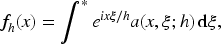
We say simply that

f_{h}

is a “localized function” at

x_{0}

. This is the basic example since

Λ_{0}

can alway be taken microlocally to such a form, and

H (x, h D_{x}; h)

h D_{x_{n}}

, where

x = (x^{'}, x_{n})

, see Section 3. Note that we can choose the amplitude

a

in equation (1.2) independent of

x

(see Hörmander, 2009, Lemma 18.2.1).

More generally, a conormal distribution $f_{h} (x) = \int^{*} e^{i x^{'} p^{'} / h} a (x, p^{'}; h) d p^{'}$ , $x = (x^{'}, x^{″}), p = (p^{'}, p^{″})$ , with respect to $N = {x^{'} = 0}$ , that is, $Λ_{0} = T_{N}^{*} R^{n} = {(x^{″}, p^{'})}$ . Again $f_{h}$ can be expressed with a new amplitude $a (x^{″}, p^{'}; h)$ not depending on $x^{'}$ .

WKB functions in Fourier representation

\begin{aligned} f_{h} (x) = \int^{*} e^{i (x p + S (p)) / h} a (x, p; h) d p, \end{aligned}

here

Λ_{0} = {(- \partial_{p} S (p), p) : p \in R^{n}}

Semi-classical distributions related with Bessel functions, microlocalized on

\begin{aligned} Λ_{0} = {x = X (φ, ψ) = φ ω (ψ), p = P (φ, ψ) = ω (ψ), φ \in R}, \end{aligned}

(1.3)

which is called the “cylinder”; here

ω \in S^{n - 1}

is the unit vector parametrized by

ψ

, see Section 5.

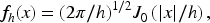
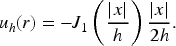
When $n = 2$ , this holds in particular for Bessel function of order 0

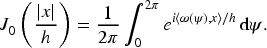
\begin{aligned} f_{h} (x) = \sqrt{\frac{2 π}{h}} J_{0} (\frac{| x |}{h}), x \in R^{2}, \end{aligned}

a radially symmetric solution of Helmholtz equation

- h^{2} Δ v - v = 0

, and follows from the integral representation:

\begin{aligned} J_{0} (\frac{| x |}{h}) = \frac{1}{2 π} \int_{0}^{2 π} e^{i ⟨ ω (ψ), x ⟩ / h} d ψ . \end{aligned}

More generally, this applies to “regular” distributions on

R^{2}

of the form

\begin{aligned} f_{h} (x) = (2 π h)^{- 1 / 2} \int_{0}^{2 π} e^{i ⟨ ω (ψ), x ⟩ / h} a (⟨ ω (ψ), x ⟩, ψ) d ψ, \end{aligned}

(1.4)

with an amplitude of the special type

a (⟨ ω (ψ), x ⟩, ψ)

. They are similar to conormal distributions in Example (2) after

x^{'}

-variables has been removed from the amplitude (see e.g. Dobrokhotov et al. (2013); Dobrokhotov et al. (2017), Section 1.5.2; Dobrokhotov et al. (2021), Section 2).

When $n = 3$ this holds also (Dobrokhotov et al., 2014) for semi-classical distributions of the form

\begin{aligned} f_{h} (x) = (2 π h)^{- 1} \int e^{i ⟨ ω (ψ), x ⟩ / h} \sin θ d θ d \tilde{ψ} = (2 π h | x |)^{- 1 / 2} J_{1 / 2} (\frac{| x |}{h}), x \in R^{3}, \end{aligned}

with

ψ = (\tilde{ψ}, θ)

the standard angular coordinates. One can also stick in an amplitude

a (⟨ ω (ψ), x ⟩, ψ)

as in equation (1.4).

$f_{h}$ identifies with a “Bessel beam” when

\begin{aligned} Λ_{0} = {(x, p) \in T^{*} R^{3} : x = (\binom{φ ω (ψ)}{ϕ}), p = (\binom{λ (ϕ) ω (ψ)}{φ λ^{'} (ϕ) + k}), ω (ψ) = (\binom{\cos ψ}{\sin ψ}), ϕ, φ \in R}, \end{aligned}

k \in R

and

λ

is a smooth positive function. Such Lagrangian distributions, with the notation

x = (x^{'}, x_{3})

, take the form

\begin{aligned} f_{h} (x) = (2 π h)^{- 1 / 2} e^{i k x_{3} / h} \int_{0}^{2 π} e^{i λ (x_{3}) ⟨ x^{'}, ω (ψ) ⟩ / h} a (λ (x_{3}) ⟨ x^{'}, ω (ψ) ⟩ + k x_{3}, x_{3}, ψ) d ψ . \end{aligned}

When

a = a (τ, α, ϕ) = \tilde{a} (α, ϕ)

and is even in

α

, we have

\begin{aligned} f_{h} (x) = \sqrt{\frac{2 π}{h}} \tilde{a} (| x^{'} |, x_{3}) e^{i k x_{3 / h}} J_{0} (\frac{λ (x_{3}) | x^{'} |}{h}) + O (h), \end{aligned}

which justifies the name “Bessel beams,” see Dobrokhotov et al. (2014b).

Airy-Bessel beams, which are known also as Berry-Balasz solution, see Berry & Balazs (1979); Dobrokhotov et al. (2014a), of the paraxial approximation of the wave equation in 3-dimensionnal space, with initial manifold

\begin{aligned} Λ_{0} = {(x, p) \in T^{*} R^{3} : x = (\binom{φ ω (ψ)}{ϕ^{2} / 2}), p = (\binom{λ ω (ψ)}{ϕ}), ω (ψ) = (\binom{\cos ψ}{\sin ψ}), ϕ, φ \in R} . \end{aligned}

Lagrangian distributions with a complex phase in the sense of Melin-Sjöstrand, see Melin and Sjöstrand (2006) equivalently a complex germ in the sense of Maslov, which are superposition of coherent states $f_{(x_{0}, ξ_{0})} (x; h) = 1 / h^{n} \exp (- ω^{2} \cdot (x - x_{0})^{2} / 2 h) \exp (i x ξ_{0} / h)$ , and $Λ_{0}$ is a strictly positive Lagrangian manifold.

Examples (1) and (4) will be extensively studied when $n = 2$ and $H_{0}$ is positively homogeneous of degree $m \geq 1$ ( $m = 1$ in Example (4)). Since $f_{h}$ in Example (5) looks like a plane wave in the direction $x_{3}$ , one could expect that Example (4) could be generalized to this case, once the eikonal coordinate has been found. Examples (6) and (7) require some special treatment and will not be considered either.

1.2. Global Parametrices for PDO’s of Principal Type and Their Semi-Classical Counterpart

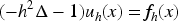
Thus our main problem is to represent the formal asymptotic solution of

\begin{aligned} (H (x, h D_{x}; h) - E) u_{h} (x) = f_{h} (x), u_{h} (x) = E_{+} (h) f_{h} (x) = \frac{i}{h} \int_{0}^{\infty} e^{- i t (H - E) / h} f_{h} (x) d t, \end{aligned}

(1.5)

in the most explicit form. Here

e^{- i t H / h}

is the propagator, so we need consider first Cauchy problem

\begin{aligned} h D_{t} v_{h} + (H (x, h D_{x}; h) - E) v_{h} = 0, v_{h} |_{t = 0} = f_{h} . \end{aligned}

(1.6)

For general

H (x, h D_{x}; h)

, we adapt the constructions of Melrose and Uhlmann (1979) to the semi-classical setting; in the case of homogeneous Hamiltonians of degree

m \geq 1

, we present formulas more globally. See Bogaevskii and Rouleux (2023a, 2023b) when

Λ_{0}

is given by (1.3), which forces

m = 1

Here we review some general concepts for solving the semi-classical PDE’s (1.5) and (1.6) in term of oscillating functions (i.e., semi-classical distributions) modulo $O (h^{\infty})$ terms, as well as their non-semi-classical analogue (for standard pseudo-differential calculus)

\begin{aligned} P (x, D_{x}) u (x) = f (x), u (x) = \int_{0}^{\infty} e^{- i t P} f (x) d t, \end{aligned}

starting from Cauchy problem

\begin{aligned} D_{t} v + P (x, h D_{x}) v_{h} = 0, v |_{t = 0} = f . \end{aligned}

In the latter case, we look for

C^{\infty}

parametrices, that is, distributions defined modulo smooth functions.

Semi-classical approximation is also called asymptotics with respect to the small parameter $h$ . This is the most natural calculus, since it is concerned with functions oscillating rapidly with respect to a given scale $h$ , but can nevertheless be smooth in $x$ . They are called semi-classical distributions. In the simplest case, these semi-classical distributions are of WKB type.

Global existence of an outgoing solution at infinity provided suitable hypotheses on Hamilton vector flow, such as Lagrangian intersection, the non-trapping and the non-return conditions, is quite involved. The main strategy in case of conormal distributions, has already been set up by Melrose and Uhlmann (1979) in the context of smooth parametrices (asymptotics with respect to smoothness) for a PDE, called sometimes Melrose-Uhlmann calculus.

The non-return condition was first formulated by Guillemin and Melrose (1979, Proposition 2.7), in constructing parametrices for hyperbolic PDE’s with a boundary (billiard problem), extending the case without a boundary (Duistermaat, & Hörmander (1972).

The non-return condition was then formulated in greater generality by Melrose and Uhlmann (1979), equation (6.5), when solving a PDE with a right-hand side. Let $Λ_{0}$ be a conic Lagrangian manifold, which we will call the “initial manifold,” and $P (x, D_{x})$ be a PDO of real principal type, with real principal symbol $p (x, ξ)$ such that the Hamilton vector field $v_{H}$ is never tangent to $Λ_{0} \cap Σ (P)$ , where $Σ (P) = {p (x, ξ) = 0}$ . Given a Lagrangian distribution $f$ microlocally supported on $Λ_{0}$ , the problem is to find $u \in D^{'} (R^{n})$ such that $P (x, D_{x}) u = f$ mod $C^{\infty}$ . Here $\partial Λ_{+} = Λ_{0} \cap Σ (P)$ plays the role of the “boundary” (generically both are of dimension $n - 1$ ). Note that the results of (Duistermaat, & Hörmander 1972) and Melrose and Uhlmann (1979) hold in a general pseudo-convex manifold $M$ , and that in (Duistermaat, & Hörmander 1972), the non-return condition is automatically satisfied. We refer to Melrose and Uhlmann (1979) for precise statements, see also Greenleaf and Uhlmann (1990), Joshi (1999), Ford et al. (2018), and Sternin and Shatalov (1983) and references therein.

The natural framework of such PDE’s has its counterpart in the semi-classical case described in equation (1.5). In particular the non-return condition (renamed as the non-refocusing condition) has received a more systematic treatment in relatively recent works (Bony, 2009; Castella, 2005; Klak & Castella, 2014).

Namely, let $Λ_{0} = T_{x_{0}}^{*} R^{n}$ be the vertical plane, and $H (x, h D_{x}) = - h^{2} Δ + V (x)$ be a semi-classical Schrödinger operator with a smooth potential $V$ with long range interaction and such that $V (x_{0}) \leq 0$ . In this case, the non-refocusing condition is characterized by the relation on $T_{x_{0}}^{*} M$ (the “return set”)

\begin{aligned} R = {(p, η) : p^{2} + V (x_{0}) = η^{2} + V (x_{0}) = 0; \exists t > 0 : X (t, p) = x_{0}, P (t, p) = η}, \end{aligned}

(1.7)

where

(X (t, p), P (t, p)) = \exp t v_{H} (x_{0}, p)

is the trajectory issued from

(x_{0}, p) \in T^{*} M

The non-refocusing condition in the restricted sense, means that $R = \emptyset$ . But the dimension of $R$ can also be taken into account. According to Castella (2005), Bony (2009), and Klak and Castella (2014), it is assumed that $\tilde{R} = {(p, η, t) \in R^{2 n + 1} : (p, η) \in R}$ is a submanifold of $R^{2 n + 1}$ of dimension less than $n - 1$ .

The non-trapping condition should also be introduced in the semi-classical setting (see also Melrose & Uhlmann, 1979, equations (6.3) and (6.4)). This is a condition on the set of trapped trajectories at energy $E_{0}$ :

\begin{aligned} K (E_{0}) = {(x, ξ) : H_{0} (x, ξ) = E_{0}, (X (t), P (t)) does not tend to infinity as | t | \to \infty} = \emptyset, \end{aligned}

where

(X (t), P (t)) = (X (t, x, ξ), P (t, x, ξ)) = \exp t v_{H_{0}} (x, ξ)

and here we can replace the non-trapping condition on the phase variables by a condition on

X (t)

alone, for example,

| X (t) | = | X (t, x, ξ) | \to \infty

| t | \to \infty

Outgoing solutions $u_{h}$ , are characterized by Sommerfeld radiation condition of the form

\begin{aligned} \frac{x}{| x |} \nabla_{x} w (x) + i \sqrt{- V (x_{0})} w (x) \to 0, | x | \to \infty, n \geq 2, \end{aligned}

(1.8)

where

w = lim_{h \to 0} w_{h}

w_{h} (x) = h^{n / 2} u_{h} (h x)

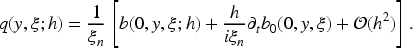
, is the unique solution of

(- Δ + V (x_{0})) w = f

, and

f_{h} (x) = h^{- n / 2} f (x / h)

. It relates in a non-trivial way the behavior of

u_{h}

at infinity with the value of the potential

V

x_{0}

. Sommerfeld radiation condition requires careful estimates on

U_{h} (t) = e^{- i t H / h}

, or

U_{h} (t) f_{h}

, along with a discussion according to the relative magnitude of

t

and

h

. The proof consists, roughly speaking, in testing

U_{h} (t) f_{h}

against some fixed

ϕ \in S (R^{n})

, and then show that

⟨ u_{h}, ϕ ⟩ \to ⟨ w, ϕ ⟩

h \to 0

. In particular, one needs to know asymptotics of

u_{h}

in a

h

-dependent neighborhood of

Λ

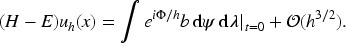
In this article instead, given $H (x, h D_{x}; h)$ and the initial Lagrangian manifold $Λ_{0}$ , we content ourselves to present, in the sense of formal asymptotics, a “closed form” for the solution of (1.5) in term of Maslov canonical operator for bi-Lagrangian distributions. So the non-refocusing and the non-trapping conditions can be largely ignored in case of formal asymptotics. By formal asymptotics (Leray, 1978) we mean that, in principle, our approximate solution is only a quasi-mode, that is, it has no reason to be equal to $E_{+} (h) f_{h}$ mod $O (h^{2})$ . In practice, however, numerical simulations show that Maslov canonical operator provides an excellent agreement with the “exact solution.”

Actually the main issue we are faced with is about existence and uniqueness of the “asymptotic solution” To fix the ideas, we can already formulate the problem as follows: How can a “formal” WKB solution approximate the solution of (1.6)? A possible answer relies on the construction of a normal form for $H (x, h D_{x}, h)$ . Assume, for instance, $H (x, h D_{x}, h)$ is self-adjoint and such that its principal symbol $H_{0} (x, p)$ is real, vanishes at $(x_{0}, p_{0})$ and $d H_{0} (x_{0}, p_{0}) \neq 0$ (by analogy with the terminology used for smoothing parametrices, we call $H (x, h D_{x}; h)$ a $h$ -PDO of real principal type near $(x_{0}, p_{0})$ ). Then $H (x, h D_{x}; h)$ is microlocally equivalent to $h D_{y_{n}}$ , that is, there is a FIO $U$ associated with the canonical transformation $κ$ such that $κ (0; 0, \dots, 0, 1) = (x_{0}, p_{0})$ (Darboux theorem), $U$ is microlocally unitary, and $‖ h D_{y_{n}} - U^{*} H (x, h D_{x}, h) U ‖ = O (h^{\infty})$ , where $‖ \cdot ‖$ is a local operator norm. This is a version of the semi-classical Egorov theorem (see e.g., Ivrii, 1998, Section 1.2). So solving (1.6) amounts to construct a solution of

\begin{aligned} h D_{t} v_{h}^{'} + h D_{y_{n}} v_{h}^{'} = 0, v_{h}^{'} |_{t = 0} = f_{h}^{'}, \end{aligned}

where

f_{h}^{'} = U^{*} f_{h}

. This PDE with constant coefficients can easily solved in the “same class” as

f_{h}^{'}

. Taking the image of

v_{h}^{'}

U

gives the suitable WKB solution of (1.6). Of course, this construction can be extended so long as

H (x, h D_{x}, h)

remains of real principal type. This is one of the basic ideas of Melrose and Uhlmann (1979), which has to be extended in the case of a (microlocal) boundary, namely to the solution of (1.5). See also Sternin and Shatalov (1983). Another ingredient for solving (1.5) is to construct an asymptotic solution in the “elliptic zone,” that is, when

H_{0} (x, p) - E \neq 0

. There we only need to invert an elliptic

h

-PDO. Gluing together the different branches of solutions follows from the “compatibility condition” (see Melrose & Uhlmann, 1979 and Section 3 below for the semi-classical case), leading here to the notion of Maslov bi-canonical operator.

In the framework of Maslov bi-canonical operator, we can, in principle, make these constructions global provided the non-trapping and the non-refocusing conditions hold.

Note that making use of the non-trapping condition only, we can ensure that our construction of Maslov bi-canonical operator can be extended to large values of $x$ , but still microlocally outside the initial manifold $Λ_{0}$ (i.e., in the case $Λ_{0}$ is the vertical plane $x = x_{0}$ , outside $x = x_{0}$ ).

Even if we had taken care of the non-trapping and the non-return conditions, we should point out that the solution to (1.5) is not unique in general. Following the principle of limiting absorption, we should introduce the auxiliary equation

\begin{aligned} (H (x, h D_{x}; h) - E + i ε) u_{h, ε} (x) = f_{h} (x), u_{h, ε} (x) = E_{+} (h, ε) f_{h} (x) = \int_{0}^{\infty} e^{- i t H / h} e^{i t (E + i ε) / h} f_{h} (x) d t, \end{aligned}

and take the limit

ε \to 0

. In case

H (x, h D_{x}; h)

is the Schrödinger operator, this is related with the fact that the limit of

u_{h, ε} (x)

, when

ε \to 0

satisfies Sommerfeld radiation condition (1.8), but in general taking the limit

ε \to 0

can be a non-trivial fact. So for simplicity again, we will ignore the limting absorption principles in this work.

To close this general introduction, we should mention again the case of parametrices for hyperbolic PDE’s with a boundary (billiard problem), which was given a new insight by Petkov and Stoyanov (2024), Petkov and Vodev (2017), and Vodev (2015, 2018, 2019, 2021). These works make use of resolvent estimates.

1.3. Lagrangian Intersection and Microlocal Green Functions

Recall the canonical 1-form on $T^{*} M$ takes (locally) the form $p d x$ ; on the extended phase-space $T^{*} (M_{x} \times R_{t})$ , (or locally on $T^{*} R^{n + 1}$ ) it is given by $p d x - E d t$ . We consider several Lagrangian manifolds:

The “initial manifold” $Λ_{0} \subset T^{*} R^{n}$ which contains ${WF}_{h} f_{h}$ . We will be concerned essentially with the “vertical plane” $Λ_{0}$ (1.2) or Bessel cylinder (1.3).

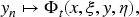
The Lagrangian submanifold in extended phase-space $T^{*} R^{n + 1}$ (denoted instead by $Λ$ by Anikin et al., 2023)

\begin{aligned} {\tilde{Λ}}_{+} = {(x, p) = g^{t} (z), t > 0, E = H (z) : z \in Λ_{0}}, \end{aligned}

(1.9)

where

g^{t} = \exp t v_{H}

is the phase flow of the Hamiltonian vector field

v_{H}

generated by

H

\begin{aligned} \dot{x} = \partial_{p} H (x, p), \dot{p} = - \partial_{x} H (x, p), \end{aligned}

(denoting

H

instead of

H_{0}

). Not to confuse

E

as a variable in (1.9) with the given value of energy in (1.5), we shall change the variable

E

E - τ

, so that

H = E

for

τ = 0

. Lagrangian manifold

{\tilde{Λ}}_{+}

contains

WF v_{h} (x, t)

, where

v_{h}

solves Cauchy problem (1.6).

The Lagrangian submanifold of $T^{*} R^{n}$ (denoted instead by $Λ_{+}$ by Anikin et al., 2023)

\begin{aligned} Λ_{+}^{E} = {z \in T^{*} R^{n} : \exists t \geq 0, z \in \exp t v_{H} (Λ_{0} \cap Σ_{E})}, \end{aligned}

(1.10)

where

Σ_{E}

is the energy surface

H = E

. Let

\partial Λ_{+}^{E} = Λ_{+}^{E} \cap Λ_{0}

be the “boundary” of

Λ_{+}^{E}

. We shall always assume Lagrangian intersection, that is,

v_{H}

is transverse to

\partial Λ_{+}^{E}

For Example (4), however, there may be points on

Λ_{+}^{E}

, where transverse intersection fails (we call them glancing points) by analogy with the problem of diffraction by obstacles, see Section 5), so we miss some informations on

u_{h}

nearby. Note that a glancing point

z_{0} \in Λ_{0}

is a critical point of

H |_{Λ_{0}}

. This is discussed by Bogaevskii and Rouleux (2023a, 2023b).

We shall assume that the amplitude $a$ defining $f_{h}$ is compactly supported in $p$ . This hypothesis is discussed in more detail by Anikin et al. (2023), Section 1.6. In particular, if $f_{h}$ is only rapidly decreasing in $p$ , then we must assume some ellipticity of $H_{0}$ at $| p | = \infty$ .

For simplicity, we restrict to the case where $\partial Λ_{+}^{E}$ is a compact, isotropic submanifold without boundary, which is certainly the case when $H_{0} (x, p)$ is elliptic. This restriction, however, is not essential (Melrose & Uhlmann, 1979) and some of our results carry to the case, where $H (x, h D_{x}; h)$ is the wave operator.

We also assume that there is no finite motion on $Σ_{E}$ , namely

\begin{aligned} | z (t) | \to \infty as t \to \infty, \end{aligned}

(1.11)

for any trajectory

z (t) = (X (t), P (t))

issued from

\partial Λ_{+}

t = 0

The non-return set $R$ in (1.7) is irrelevant if we content ourselves with the asymptotics of $u_{h} (x)$ microlocally in a compact set outside $\partial Λ_{+}^{E}$ . For instance, if $Λ_{0} = T_{x_{0}}^{*} M$ , we shall compute $u_{h} (x)$ , locally uniformly in any compact set $K \subset M ∖ {x_{0}}$ , as $h \to 0$ . A first improvement would consist in removing only a $h^{δ}$ -neighborhood of $x_{0}$ for some $0 < δ < 1$ , this we have sketched by Anikin et al. (2017), Theorem 2.

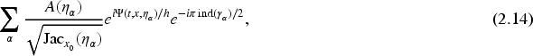
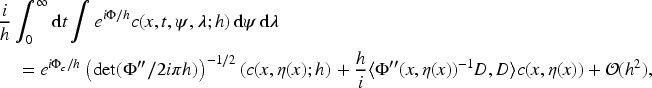
Our main goal is to represent formally (1.5) as a superposition

\begin{aligned} u_{h} (x) = \frac{i}{h} \int_{0}^{\infty} [K_{{\tilde{Λ}}_{+}}^{h} b] (x) d t + O (h), \end{aligned}

(1.12)

where

[K_{{\tilde{Λ}}_{+}}^{h} b] (x, t)

is Maslov canonical operator associated with

{\tilde{Λ}}_{+}

, and

b

is an amplitude depending linearly from the amplitude

a

defining

f_{h}

The relevant contributions to this integral come from $t = + \infty$ , $t = 0$ and the critical points $t \in] 0, + \infty [$ .

The contribution of $t = + \infty$ is excluded by (1.11). If we do not have glancing points, then $Λ_{+}^{E}$ is a smooth Lagrangian submanifold. We need to take into account $t = 0$ in formula (1.12). If the initial manifold $Λ_{0}$ is the vertical then this contribution is zero outside of $x_{0}$ . Otherwise (as is the case $Λ_{0}$ is Bessel cylinder), the contribution of $t = 0$ is not zero but maybe of small order (as $\sqrt{h}$ ). But if $f_{h}$ has compact support, then the contribution of $t = 0$ is zero outside $supp (f_{h})$ .

The critical points $t \in] 0, + \infty [$ give of course the main contributions to (1.12), and give in principle all possible types of Lagrangian singularities in $R^{n}$ , microlocally outside $Λ_{0}$ . This will be investigated in detail in Sections 4 and 5 for a particular type of Hamiltonian which allows to construct quite explicit “global” asymptotic solutions.

In case $Λ_{0} = T_{x_{0}}^{*} M$ is the vertical plane, (1.11) can be replaced by $| X (t) | \to \infty$ as $t \to + \infty$ , and the measure on $Λ_{+}$ factorizes as $d μ_{+} = d μ_{0}^{E} \land d t$ , where $d μ_{0}^{E}$ is the measure on $\partial Λ_{+}^{E}$ , see Anikin et al. (2023, Theorem 2). The accuracy $O (h)$ in (1.12) can improve to $O (h^{\infty})$ , see Anikin et al. (2023, Theorem 4), and also Sternin and Shatalov (1983).

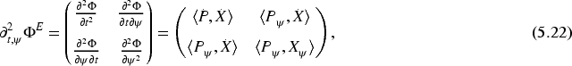
One of our claims is to express $\int_{0}^{\infty} d t [K_{Λ_{+}}^{h} b]$ as some “bi-canonical operator” $[K_{Λ_{0}, Λ_{+}}^{h} (σ, σ^{+})]$ acting on pairs of symbols $(σ, σ^{+})$ depending linearly on $b$ , resp. the boundary-part and the wave-part symbol of $u_{h}$ , which we call a bi-Lagrangian (semi-classical) distribution. This follows from a symbolic semi-classical calculus similar to Melrose and Uhlmann (1979).

For simplicity, we shall ignore throughout Maslov indices. Corrections to the asymptotics due to Maslov indices follow, for instance, easily from Arnold (1967, 1976), Bates and Weinstein (1997, Section 4); Souriau (1976), Ivrii (1998), Dobrokhotov et al. (2017), Dobrokhotov and Rouleux (2011), and Esterlis et al. (2014). See also Anikin et al. (2023).

1.4. Main Results

General case.

In Section 3, we translate the setting of classical pseudo-differential calculus elaborated by Melrose and Uhlmann (1979) to the semi-classical one, and make some statements more precise. By Proposition 3.2 below, near any

z \in \partial Λ_{+}^{E}

we are reduced microlocally to the case where

Λ_{0} = T_{0}^{*} R^{n}

, and

Λ_{+}^{E} = L_{+}^{0}

is the flow out of the “model Hamiltonian”

H_{0} = η_{n}

in energy surface

η_{n} = 0

. In Proposition 3.5, we show that

H (x; h D_{x}; h) - E

can be taken microlocally near

L_{+}^{E}

to its normal form

h D_{y_{n}}

by conjugating with a

h

-FIO. So without loss of generality, we may assume that, after some canonical transformation,

Λ_{0} = T_{x_{0}}^{*} M

. We have the following theorem:

Theorem 1.1
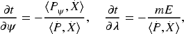
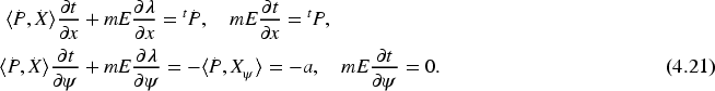
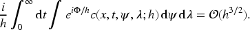
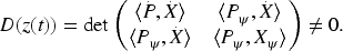
Let $H (x, p; h) \in S_{m}^{0} (T^{} M)$ (not necessarily homogeneous with respect to p). Assume the vertical plane $Λ_{0} = T_{x_{0}} M$ , and $Σ_{E} = {H_{0} (x, p) = E}$ , where $E$ is a non-critical energy level, intersect transversally along the compact isotropic manifold $\partial Λ_{+}^{E}$ . Assume $| X (t) | \to \infty$ as $t \to \infty$ for all initial conditions $(X (0), P (0)) \in \partial Λ_{+}^{E}$ . Let also $f_{h}$ be a semi-classical distribution microlocalized on $Λ_{0}$ of the form (1.2), with $x_{0} = 0$ (to fix the ideas), and where we can assume the symbol is independent of $x$ . Then there is $ε_{0} > 0$ such that the equation $(H (x, h D_{x}) - E) u_{h} (x) = f_{h} (x) + O (h^{2})$ can be solved in the form (1.12) for $0 < | x - x_{0} | < ε_{0}$ , locally uniformly for $h > 0$ small enough.

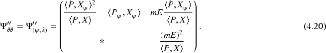
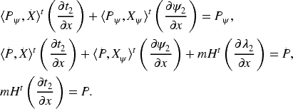
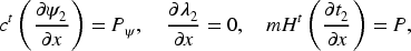
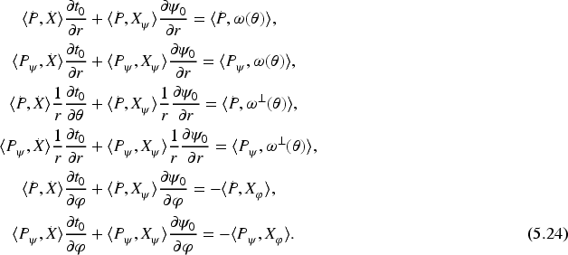
Moreover, there are symbols $(σ, σ^{+})$ , such that in local coordinates $σ (ξ; h) = 1 / ξ_{n} b (ξ; h)$ , $σ^{+} (ξ; h) = 2 i π b (ξ^{'}, 0; h)$ verify the compatibility condition
$\begin{aligned} lim_{ξ_{n} \to 0} ξ_{n} σ (ξ^{'}, ξ_{n}; h) = σ^{+} (ξ^{'}, 0; h), \end{aligned}$
(1.13)
and such that $u_{h}$ can be represented by Maslov “bi-canonical operator,” see (3.28) as
$\begin{aligned} u_{h} (x) = [K_{Λ_{0}, Λ_{+}^{E}}^{h} (σ, σ^{+})] (x) . \end{aligned}$
We have the commutation relation
$\begin{aligned} H (x, h D_{x}; h) [K_{Λ_{0}, Λ_{+}^{E}}^{h} (σ, σ^{+})] (x; h) = [K_{Λ_{0}, Λ_{+}^{E}}^{h} ((H - E) σ, 0)] (x; h) + O (h^{2}) = f_{h} (x) + O (h^{2}), \end{aligned}$
(1.14)
for $0 < | x - x_{0} | < ε_{0}$ , locally uniformly for $h > 0$ small enough.

We stress that this representation holds in a punctured neighborhood of $x_{0}$ , that is, is not uniform in $x$ near $x_{0}$ , since we have neglected the non-return condition.

However, since the Hamiltonian vector field $v_{H}$ remains transverse to $Λ_{t} = g^{t} (Λ_{0})$ for all $t$ , the condition $| x - x_{0} | < ε_{0}$ is not really a restriction. Namely, using local charts for Maslov “bi-canonical operator” as in the case of Maslov canonical operator associated with the homogeneous equation (see Section 3.2 below), the asymptotic solution $u_{h}$ can be made global outside $x_{0}$ . See also Anikin et al. (2023, Theorem 4).

The remainder term $O (h^{2})$ in (1.14) can be improved by considering higher-order transport equations and using the compatibility condition (1.13).

Maslov “bi-canonical operator” is some operator version of the “compatibility condition” by Melrose and Uhlmann (1979), formula (2.10) and Section 4. It encompasses the parametrices both in the elliptic region $H (x, p) \neq E$ and in the hyperbolic region $H (x, p) = E$ (see Theorems 1 and 2 by Anikin et al., 2023).
Hamiltonian $H_{0}$ is homogeneous of degree $m$ with respect to $p$ and $Λ_{0}$ is the vertical plane.
The previous result is not very useful from the point of view of applications, since it does not provide a “close form” for $u_{h}$ . Much more information is available when Hamiltonian $H_{0}$ is homogeneous of degree $m$ with respect to $p$ , due to the relations $⟨ P (t, ψ), \dot{X} (t, ψ) ⟩ = m H$ and $⟨ P (t, ψ), X_{ψ} (t, ψ) ⟩ = 0$ (Huygens principle). We have chosen coordinates $(λ, ψ)$ on $Λ_{0}$ , $λ$ a “radial coordinate” such that $λ = 1$ on $H = E$ and $ψ \in R^{n - 1}$ coordinates along $\partial Λ_{+}^{E}$ , we can think of as angles parametrizing the $(n - 1)$ -sphere.

Lagrangian intersection always holds on $Λ_{0}$ , for if $\partial_{p} H (x_{0}, p) = 0$ , Euler identity gives $0 = ⟨ \partial_{p} H (x_{0}, p), p ⟩ = m H = m E$ which contradicts $E \neq 0$ . We will, therefore, assume the non-trapping condition (in $x$ ) $| X (t) | \to \infty$ , $t \to + \infty$ .

Note that such a symbol is not suitable for pseudo-differential calculus when $m$ is not an even integer, because of the singularity at $p = 0$ , but this is harmless if $(x_{0}, 0) \notin {WF}_{h} (f_{h})$ .

A particular case of these Hamiltonians is the “conformal metric” given by the following equation:
$\begin{aligned} H (x, p) = | p |^{m} \frac{1}{ρ (x)}, \end{aligned}$
(1.15)
where $ρ$ be a smooth positive function on $M$ , $m \geq 1$ . In case $m = 2$ , $H (x, p)$ identifies, through Maupertuis-Jacobi correspondence, with Helmholtz Hamiltonian in a non-homogeneous medium with refraction index $n (x) > 0$ such that $n {(x)}^{2} = ρ (x)$ . We shall pay a great attention to this Hamiltonian, for which computations are most explicit.

Recall that a focal point* for a Lagrangian embedding $ι : \tilde{Λ} \to T^{} M$ (where $\tilde{Λ}$ is either $Λ$ , $Λ_{t} = \exp t v_{H} (Λ)$ , or $Λ_{+}^{E}$ ) is a point $z \in \tilde{Λ}$ such that $d π_{x} : \tilde{Λ} \to M$ has rank $< n$ . The set of focal points is denoted by $F (\tilde{Λ})$ . Recall also that there exists a covering of $\tilde{Λ}$ by canonical charts $U$ , where $rank d π_{x} (z) \geq k$ for all $z \in U$ . These $U$ for which $k = n$ are called regular* charts, and those for which $k < n$ singular charts.

At least for $0 < | x - x_{0} |$ small enough, that is, $0 < t$ small enough, using at most two canonical charts (depending if $X_{ψ} (t, ψ) = 0$ or not) we can construct $v_{h}$ solution of Cauchy problem (1.6), and hence $u_{h}$ by integration with respect to $t$ . To this end, we introduce eikonal coordinates (see Section 2), and a generating family for $Λ_{+}^{E}$ as (see (4.5)):
$\begin{aligned} Φ (x, t, ψ, λ) = m E t + λ ⟨ P (t, ψ), x - X (t, ψ) ⟩ . \end{aligned}$
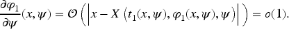
The “ $θ$ -variables” are thus $(t, ψ, λ)$ . This defines the 1-jet along the critical set $x = X (t, ψ), λ = 1$ of the solution of Hamilton-Jacobi equation associated to (1.6). This yields (see equations (3.7) and (4.14)) an (inverse) density on $Λ_{+}^{E}$ , given by $μ_{+} = F [Φ, d y] = m E det (P, P_{ψ})$ ( $d y$ being Lebesgue measure on the critical set) and non-vanishing precisely when $Φ (t, x, ψ, λ)$ is a non-degenerate phase function, see Propositions 4.3 and 4.8. This holds at least for small $t$ . For larger $t$ , the non-vanishing of $m E det (P, P_{ψ})$ will only be assumed.
Theorem 1.2
Let $n = 2$ , and $H_{0} (x, p)$ be positively homogenenous of degree $m \geq 1$ . Let $r_{0} > 0$ such that
$\begin{aligned} \forall t > 0, \forall ψ \in R : [| X (t, ψ) | < r_{0} ⟹ det (P (t, ψ), P_{ψ} (t, ψ)) > 0], \end{aligned}$
(this holds for $t > 0$ small). Then there is $ε_{0} > 0$ such that the equation $(H (x, h D_{x}) - E) u_{h} (x) = f_{h} (x) + O (h^{3 / 2})$ can be solved in the form of the following equation:
$\begin{aligned} u_{h} (x) = \frac{i}{h} \int_{0}^{\infty} d t \int e^{i Φ (x, t, ψ, λ) / h} b (x, t, ψ, λ) d ψ d λ, \end{aligned}$
(1.16)
for $0 < | x - x_{0} | < ε_{0}$ , locally uniformly for $h > 0$ small enough.

Moreover, we can decompose
$\begin{aligned} \int_{0}^{\infty} d t [K_{Λ_{t}}^{h} b] (x) = \int_{0}^{\infty} d t [K_{Λ_{t}}^{h} (χ_{1} b)] (x) + \int_{0}^{\infty} d t [K_{Λ_{t}}^{h} (χ_{2} b)] (x), \end{aligned}$
(1.17)
where $χ_{1} + χ_{2} = 1$ is a partition of unity subordinated to a chart $U_{1}$ , where $X_{ψ} \neq 0$ and a (singular) chart $U_{2}$ , where $X_{ψ} = 0$ , $χ_{2} \equiv 1$ near $| X_{ψ} | \leq \frac{1}{3}$ , and $χ_{1} \equiv 1$ near $| X_{ψ} | \geq \frac{2}{3}$ , both contributions being discussed in Sections 4.4 and 4.5 below.

We do not attempt here to formulate the result in terms of bi-canonical Maslov operator as in Theorem 1.1. Note the loss of accuracy ( $O (h^{3 / 2})$ ) instead of $O (h^{2})$ in Theorem 1.1. In Section 2.3, we discuss (somewhat informally) the case where $x$ has several pre-images under $π_{x} : Λ_{+}^{E} \to M$ .

By constructing (1.5) and (1.6), we mean also determining the Lagrangian singularities of $u_{h}$ . They are revealed when reducing the number of “ $θ$ -variables” in the oscillating integral $\int_{0}^{\infty} d t [K_{Λ_{t}}^{h} b] (x)$ . We get virtually any kind of Lagrangian singularity, but because of homogeneity of $H$ with respect to $p$ , it is convenient to introduce another classification in $T^{} M$ , which clarifies the construction of $u_{h}$ .
Definition 1.3
Let $H$ be positively homogeneous of degree $m$ with respect to $p$ . We call a point $z = (x, p)$ such that $- \partial_{x} H (z) \neq 0$ an ordinary* point if $⟨ - \partial_{x} H (z), p ⟩ \neq 0$ , and a special point otherwise. If $- \partial_{x} H (z) = 0$ we call $z$ a residual point.

Here are some examples: (1)
For Tricomi Hamiltonian, $H (x, p) = x_{2} p_{1}^{2} + p_{2}^{2}$ , the residual points are those for $p_{1} = 0$ , the special points those for $p_{1} \neq 0$ but $p_{2} = 0$ , and the ordinary points those for $p_{1} p_{2} \neq 0$ . Tricomi operator is used as a model for diffraction. This model extends to the 3D case as $H (x, p) = - p_{2}^{2} + p_{1} p_{3} + x_{2} p_{1}^{2}$ .
(2)
For Métivier Hamiltonian, $H (x, p) = p_{1}^{2} + (x_{1}^{2} + x_{2}^{2}) p_{2}^{2}$ , the residual points are given by $p_{2} = 0$ or $x = 0$ , the special points by $p_{2} \neq 0$ and $x \neq 0$ , but $⟨ x, p ⟩ = 0$ , and the ordinary points by $⟨ x, p ⟩ p_{2} \neq 0$ . Métivier operator provides a counter-example for analytic hypo-ellipticity.
(3)
Let $H$ be the “conformal metric” given by (1.15). The residual points are the critical points of $ρ$ ; at a special point, $⟨ \nabla ρ, p ⟩ = 0$ , that is, $v_{H}$ is tangent to the level curves of $ρ$ . This is our main example here.
We denote by $S (Λ_{+}^{E})$ the set of special points on $Λ_{+}^{E}$ . We shall partition points $z \in Λ_{+}$ according to the following values: (1) $z$ is a focal (or non-focal) point; (2) $z$ is a special (or ordinary, or residual) point. Thus each canonical chart splits again into ordinary, special or residual points. Assume $n = 2$ for simplicity.

Let $x = X (t, ψ)$ , and $⟨ - \partial_{x} H (x, p), \partial_{p} H (x, p) ⟩ \neq 0$ at $(x, p) = z (t) = (X (t, ψ), P (t, ψ))$ . Then
$\begin{aligned} \partial_{t} Φ (t, x, ψ, λ = 1) = 0 ⟹ \partial_{t}^{2} Φ (t, x, ψ, λ = 1) \neq 0, \end{aligned}$
(1.18)
so that we can perform asymptotic stationary phase in $t$ to simplify (1.5) at $x = X (t, ψ)$ . This holds when $H$ is of the form (1.15) and $z (t)$ is an ordinary point. Likewise, if several values of parameters $t$ contribute, we sum over such $t$ ’s. Then $Φ (x, t, ψ, λ = 1)$ reduces to a phase function $Ψ (x, ψ)$ and we can further reduce the number of variables in a standard way, according to the fact that $z (t)$ is a focal point or not. When $⟨ - \partial_{x} H (x, p), \partial_{p} H (x, p) ⟩ = 0$ but $- \partial_{x} H (x, p) \neq 0$ , we have
$\begin{aligned} \partial_{t} Φ (t, x, ψ, λ) = \partial_{λ} Φ (t, x, ψ, λ) = 0 ⟹ det Φ_{(t, λ), (t, λ)}^{″} (t, x, ψ, λ) \neq 0, \end{aligned}$
(1.19)
where $λ$ is constrained to be equal to 1 on the critical set $C_{Φ}$ , so that we can perform asymptotic stationary phase with respect to $(t, λ)$ . Then $π_{x} : Λ_{+}^{E} \to T^{} R^{n}$ has rank 1 if $z (t)$ is a special point or rank 2 otherwise, see Proposition 4.6(ii). Note that $Λ_{+}^{E}$ never turns vertical, since $\partial_{p} H (x, p) \neq 0$ on $H = E$ .

In this generality, we only succeed (see Proposition 4.6) to describe the contribution to (1.5) (by asymptotic stationary phase) of short times $t$ (“near field”), that is, so long as $F [Φ, d y] = m E det (P, P_{ψ})$ $\neq 0$ , but this is actually sufficient to compute $u_{h}$ microlocally near $Λ_{0}$ , when $x \neq x_{0}$ .
$H_{0}$ is the “conformal metric” $H_{0} (x, p) = \frac{| p |^{m}}{ρ (x)}$ and $Λ_{0}$ is the “vertical plane.”
Using that $P (t, ψ)$ is parallel to $\partial_{p} H (x, p)$ we get more complete results in this case. If $ρ$ is bounded, a sufficient condition for (1.12) is that energy $E$ is non-trapping. The following stronger condition excludes natural potentials having a limit as $| x | \to \infty$ , as shows the example $ρ (x) = ρ_{0} + ⟨ x ⟩^{- ε}$ . However it turns out to be convenient from the point of vue of the following:
Definition 1.4
We say that $ρ$ has the defocusing condition* iff
$\begin{aligned} G (ρ) (x, p) = ⟨ \nabla^{2} ρ (x) \cdot p, p ⟩ + \frac{| \nabla ρ (x) |^{2}}{m ρ (x)} | p |^{2} > 0, \forall (x, p) \in {H_{0} = E} . \end{aligned}$
(1.20)

In particular if $ρ$ has a critical point, this is a non-degenerate minimum. Under defocusing condition (1.20), if $z (s)$ is a special point along some bicharacteristic $γ$ issued from $Λ_{0}$ , then for all $t > s$ , $z (t) \in γ$ is an ordinary point. We expect that (1.20) is related to the non-trapping condition (1.12), and provides an information on the “return set” in (1.7), for example, $R = \emptyset$ . It also implies that special and residual points are “exceptional” compared to ordinary points, in the same way singular points are “exceptional” with respect to regular points. This allows a natural subdivision of canonical charts into ordinary and special (residual) points, so we can speak of a regular-ordinary chart, or regular-special chart, and so on. The main results are summarized in Proposition 4.11.
Remark 1.5
In case (1.15) with $m = 1$ and $f_{h} = 0$ (scattering problem), the asymptotic solution of $H (x, h D_{x}) u_{h} = E u_{h}$ has been constructed by Dobrokhotov et al. (2013, Example 6), in term of Bessel functions.

$Λ_{0}$ is “Bessel cylinder” $(1.3)$ , and $m = 1$ .
To the former “ $θ$ -variables” $(t, ψ, λ)$ , one has now to add $φ$ as a parameter. Note that $Λ_{0}$ has a Lagrangian singularity at $φ = 0$ . This is the most technical part of the article, and the results are only partial, because we are ignoring glancing points. It is necessary here to assume $m = 1$ . For $m = 1$ , Euler identity shows that the 1-form $p d x - E d t$ vanishes on $Λ_{+}$ . We are led to assume $m = 1$ . For simplicity, we shall also assume essentially that $H$ is of the form (1.15) with $ρ$ radially symmetric.

Due to possible glancing points, we cannot formulate a global result in term of Maslov canonical operator as in Theorem 1.2. For an Hamiltonian positively homogeneous of degree 1 in the $p$ variables, we content ourselves with computing the phase and density on $Λ_{+}^{E}$ , so our results are most complete in case of the conformal metric. This simplifies further in case of a radially symmetric conformal metric. We refer to Section 5 for detailed statements.
1.5. Outline of the Article

In Section 2, we first construct eikonal coordinates on $Λ_{+}^{E}$ when $H_{0} (x, p)$ is positively homogeneous of degree $m$ , and $Λ_{0}$ is either the vertical plane, or Bessel cylinder. Then we discuss some well-known facts about the extension of the solution of Cauchy problem (1.6) for large $t$ . In particular, we examine the case where there are several branches of $Λ_{+}^{E}$ lying over $x$ , that is, $π_{x} (X (t, ψ), P (t, ψ)) = x$ , leading to Van-Vleck formula. Following Colin de Verdière (2005), Guillemin and Sternberg (1977), and Guillemin and Sternberg (2013) we then focus to the case when $H_{0}$ defines a metric, according to $m = 1$ (Finsler metric, or Randers symbol), or $m > 1$ .

In Section 3, we prove Theorem 1.1. We start to recall some basic facts on Maslov theory. Then we sketch its generalization to bi-Lagrangian distributions, following mainly Melrose and Uhlmann (1979), where $H$ is taken microlocally to its normal form $h D_{x_{n}}$ on a non-critical energy surface. We make also the results of Melrose and Uhlmann (1979) more precise and adapted to asymptotics with respect to the small parameter $h$ . Thus we can construct $u_{h} (x)$ microlocally outside $\partial Λ_{+}^{E}$ , and locally uniformly with respect to $h$ . We end up by computing explicitely $u_{h}$ when $n = 2$ , $H = - h^{2} Δ$ and $f_{h}$ is compactly supported, and verify that $u_{h}$ can be written as the sum of two terms, microlocally supported on $Λ_{0}$ and $Λ_{+}^{E}$ , respectively.

We start in Section 4 to recall from Dobrokhotov et al. (2014b, 2017), the matrix $\tilde{n} \times \tilde{n}$ matrix $M (\tilde{ϕ}, \tilde{ψ})$ defined on a local chart of a Lagrangian manifold $\tilde{Λ}$ , whose determinant turns out to be the (inverse) density on $\tilde{Λ}$ . It will be most useful in Section 5. Then we define the phase function from which compute directly the (inverse) density $F [Φ, d y] |_{C_{Φ}}$ on $Λ_{+}^{E}$ . Later on we restrict to the 2D case. In Section 4.3, assuming this density is non-zero, or equivalently, that $Φ$ is a non-degenerate phase function in the sense of Hörmander, we investigate some configurations of $Λ_{+}^{E}$ in $T^{*} M$ (according to $X_{ψ} = 0$ or $X_{ψ} \neq 0$ ) and describe more closely the corresponding Lagrangian singularities (focal points) in the chart, where $X_{ψ} \neq 0$ . We relate focal points with ordinary, special or residual points. In Section 4.4, we complete the first-order asymptotics by considering the transport equations, and prove Theorem 1.2. In Section 4.5, we specialize further to the case of the “conformal metric,” using also the defocusing condition (1.20), which allows a more complete description of focal points.

Section 5 is the most technical and sketchy part, since we do not take glancing point into account. In Section 5.1, we give necessary and sufficient for a point of the “cylinder” (1.3) be glancing with respect to $v_{H_{0}}$ . In particular, we show that a glancing point at $t = 0$ is also a special point. Then we describe the parametrization of $\partial Λ_{+} (τ)$ provided this is a closed manifold without boundary. We compute the matrix $M (t, φ, ψ, τ)$ we introduced already in Section 4, and show that we should take $m = 1$ so that its determinant identifies with the density on $Λ_{+}$ . All computations should be carried in the extended phase-space $T^{*} (M \times R_{t})$ .

In the Appendix, we prove the density is non-vanishing near focal points in the case of the “conformal metric.”

1.6. Some Open Problems

$∙$
Semi-classical structure of the Green function outside a $h^{δ}$ -neighborhood of $Λ$ .
$∙$
Other types of initial Lagrangian manifolds, for example, more general Bessel or Airy-Bessel beams, for which the initial manifold $Λ_{0}$ is similar to the Bessel cylinder.
$∙$
Structure of the Green function near residual points, in particular glancing points, where Lagrangian intersection fails to be transverse, see Bogaevskii and Rouleux (2023b).
$∙$
Hyperbolic equations ( $\partial Λ_{+}$ non-compact).
$∙$
Case of multiple characteristics, involving Lagrangian manifolds with boundary $\partial Λ_{+}$ and corner $c Λ_{+}$ (Melrose & Uhlmann, 1979).
$∙$
Complex phases as in Example (7).
$∙$
Nonlinear PDE’s: Melrose-Uhlmann calculus has been used in the study of propagation of singularities for nonlinear wave equations, see Uhlmann and Zhai (2021), and it would be natural to try the semiclassical analogue in the analysis of oscillatory solutions, as in the work of Joly-Métivier-Rauch (1996, 2021).

2. Hamiltonians and Phase Functions

In this section, we consider integral manifolds for positively homogeneous Hamiltonians on $T^{*} M ∖ 0$ , which is the first step in constructing semi-classical Green kernels. We discuss first general facts (eikonal coordinates and Hamilton-Jacobi (HJ) equation), but more specific points will be discussed in Sections 4 and 5. Basic references are Arnold (1967, 1976), Hörmander (2009), and Guillemin and Sternberg (1977, 2013).

2.1. Eikonal Coordinates

First, we recall some general facts about canonical coordinates on Lagrangian manifolds, see Dobrokhotov et al. (2013, 2017). Let $ι : L \to T^{*} M$ be a smooth embedded Lagrangian manifold. We write $(x, p) = ι (α) = (X (α), P (α))$ , where $α$ is a local coordinate on $L$ . The 1-form $p d x$ is closed on $L$ , so is locally exact, and $p d x = d S$ on any simply connected domain $U$ (the so-called canonical chart). Such a $S$ is called an eikonal (or action) and is defined up to a constant. If $p d x = d S \neq 0$ on $U$ , $ϕ = S$ can thus be chosen as a coordinate on $U$ , that is, a local coordinate on $L$ , and completed by coordinates $ψ \in R^{n - 1}$ such that

\begin{aligned} ⟨ P, \partial_{ϕ} X ⟩ = 1, ⟨ P, \partial_{ψ} X ⟩ = 0, ⟨ \partial_{ψ} P, \partial_{ϕ} X ⟩ = ⟨ \partial_{ϕ} P, \partial_{ψ} X ⟩ . \end{aligned}

(2.1)

This holds true if

L

is projectable on

U

, that is,

U

of rank

n

, but this condition is not necessary. Namely, consider a local chart

U

of rank

k = 1

, and let

α = (ϕ, ψ)

ϕ \in R

ψ \in R^{n - 1}

, so that

L

is defined by

x = X (ϕ, ψ)

p = P (ϕ, ψ)

, then

\begin{aligned} d ϕ = ⟨ P (ϕ, ψ), d X (ϕ, ψ) ⟩, \end{aligned}

(2.2)

and

ϕ

is an eikonal on

L

. See Dobrokhotov et al. (2017), Section 1.4.3.

We shall deal with elliptic positively homogeneous Hamiltonians of degree $m \geq 1$ with respect to $p$ on the cotangent bundle $T^{*} M ∖ 0$ ( $M = R^{n}$ for simplicity), and eventually restrict to “conformal metrics” to get most explicit results. In this section, we write $H$ for $H_{0}$ .

Example 2.1

(1)

$m = 2$ if $H (x, p)$ is a geodesic flow associated with a Riemannian metric $d s^{2} = g_{i j} (x) d x^{i} \otimes d x^{j}$ . In the Riemannian case, when $E = 1$ , geodesics are parametrized by the arc-length.

(2)

$m = 1$ if $H (x, p)$ is a “Randers symbol,” associated with a Finsler metric (Taylor, 2009), Dobrokhotov and Rouleux (2012), and reference therein.

(3)

$H$ is of the form (1.15) with $m \geq 1$ . Hamilton equations $(\dot{x}, \dot{p}) = v_{H} (x, p)$ then read

\begin{aligned} \dot{x} & = \partial_{p} H = m | p |^{m - 1} \frac{1}{ρ (x)} \frac{p}{| p |}, \dot{p} = - \partial_{x} H = | p |^{m} \frac{\nabla ρ (x)}{ρ {(x)}^{2}} . \end{aligned}

(2.3)

Our most complete results hold for such Hamiltonians with

n = 2

$∙$ Case of the “vertical plane.” When $H$ is positively homogeneous of degree $m$ with respect to $p$ , and $Λ_{0}$ is the vertical plane, $v_{H}$ is always transverse to $Λ_{0}$ when $E \neq 0$ , that is, there are no glancing points.

Let $L = Λ_{+}^{E}$ be the flow-out of $H$ with initial data on $Λ_{0} = T_{x_{0}}^{*} M$ . Thus $L$ is the union of maximally extended bicharacteristics starting at $Λ_{0}$ , and $ι : Λ_{+}^{E} \to T^{*} M$ a Lagrangian immersion.

Let also $ψ \in R^{n - 1}$ be smooth coordinates on $\partial Λ_{+}^{E}$ , which we complete by $- τ$ , the dual coordinate of $t$ , so that $\partial Λ_{+}^{E}$ is given in $Λ_{0}$ by $τ = 0$ , and in $Λ_{+}^{E}$ by $t = 0$ .

In the special case $H (x, p) = | p |^{m} / ρ (x)$ , we have $P (ψ, τ) = | P |_{τ} ω (ψ)$ , with $ω (ψ) \in S^{n - 1}$ ,

\begin{aligned} | P |_{τ} = (H ρ (0))^{1 / m} = {((E - τ) ρ (0))}^{1 / m} . \end{aligned}

(2.4)

The sections are defined as follows: for small

τ

, let

Λ_{+} (τ) = Λ_{+}^{E - τ}

be the Lagrangian manifold in the energy shell

τ + H (x, p) = E

issued from

Λ_{0}

t = 0

. We consider the isotropic manifold

\partial Λ_{+} (τ) = Λ_{0} \cap Λ_{+} (τ)

, viewing

Λ_{+} (τ)

as a manifold with boundary. When

τ = 0

, we simply write

Λ_{+} (0) = Λ_{+}^{E}

For $t \geq 0$ , let $Λ_{t} = \exp t v_{H} (Λ)$ , we have the group property $Λ_{t + t^{'}} = \exp t v_{H} (Λ_{t^{'}})$ for all $t, t^{'} \geq 0$ .

We define in a similar way the family of isotropic manifolds $\partial Λ_{t} (τ) = \exp t \partial Λ_{+} (τ) = Λ_{t} \cap Λ_{+} (τ)$ .

We compute the eikonal $S$ on $Λ_{+} (τ)$ by integrating along a piecewise $C^{1}$ path connecting the base point, say $(x_{0}, 0) \in Λ_{0}$ (where $d x = 0$ ) to $(x_{0}, P (ψ)) \in \partial Λ_{+} (τ)$ , $ψ \in R^{n - 1}$ , followed by the integral curve $x = X (t, ψ), p = P (t, ψ)$ of $v_{H}$ starting at $(x_{0}, P (ψ))$ , where $d S = p d x |_{Λ_{+} (τ)} = ⟨ P (t, ψ), d X (t, ψ) ⟩$ . Because $Λ_{+} (τ)$ is Lagrangian, $S$ does not depend on the choice of the base point. Since $S (0, ψ) = Const . = S_{0}$ on $Λ_{0}$ , we get

\begin{aligned} S (t, ψ) & = S (0, ψ) + \int_{(0, ψ)}^{(t, ψ)} p d x |_{Λ_{+}} = S (x_{0}, ψ) + \int_{(0, ψ)}^{(t, ψ)} P (s, ψ, τ) d X (s, ψ, τ) \\ = S_{0} + \int_{0}^{t} ⟨ P (s, ψ, τ), \dot{X} (s, ψ, τ) ⟩ d s . \end{aligned}

(2.5)

By Hamilton equations and Euler identity,

⟨ P (s, ψ, τ), \dot{X} (s, ψ, τ) ⟩ = ⟨ P, \partial_{p} H ⟩ = m H = m (E - τ)

. Now

S (t, ψ) = S_{0} + m (E - τ) t = S_{0} + m H t

is the action on

Λ_{+} (τ)

, and the eikonal coordinate is just

S (t, ψ) = m H t

up to a constant

S_{0}

, and we may set

S_{0} = 0

. Restricting to

Λ_{+} (τ)

we get

d S = d (m (E - τ) t) = m (E - τ) d t

, or

\begin{aligned} m (E - τ) d t = ⟨ P (t, ψ, τ), d X (t, ψ, τ) ⟩ = ⟨ P (t, ψ, τ), \dot{X} (t, ψ, τ) ⟩ d t + ⟨ P (t, ψ, τ), X_{ψ} (t, ψ, τ) ⟩ d ψ, \end{aligned}

(2.6)

and it follows (Huygens’ principle) that:

\begin{aligned} ⟨ P (t, ψ, τ), \dot{X} (t, ψ, τ) ⟩ = m H, ⟨ P (t, ψ, τ), \partial_{ψ} X (t, ψ, τ) ⟩ = 0 . \end{aligned}

(2.7)

We will denote for short

(X, P) = (X (t, ψ, τ), P (t, ψ, τ))

X (t, ψ), P (t, ψ)

when

τ = 0

. This is called the leading front.

$∙$ Case of “Bessel cylinder.” Even for positively homogeneous $H$ of degree $m$ with respect to $p$ , there may be glancing points, but $Λ_{+}^{E}$ is still an immersed Lagrangian manifold away from the trajectories starting at the glancing points. In this work, we restrict to local charts where $Λ_{+}^{E}$ is immersed, glancing intersection being considered by Bogaevskii and Rouleux (2023a, 2023b).

Let $L = Λ_{0}$ , then $p d x |_{Λ_{0}} = d φ$ , which shows that $φ$ is the eikonal on $Λ_{0}$ .

Let $H$ be homogeneous of degree $m = 1$ with respect to $p$ , and $L = Λ_{+}$ be the flow out of $Λ_{0}$ by $v_{H}$ in the extended phase-space. According to Euler identity, $\dot{S} = p \dot{x} - H = p \partial_{p} H - H = 0$ along the trajectories, the eikonal on $Λ_{+}$ is again $S = φ$ , and $(φ, ψ, t) = φ$ are eikonal coordinates. This results also from the fact that $v_{H}$ preserves $p d x$ on $Λ_{+}$ (see also (2.15) below).

Let $L = Λ_{+} (τ)$ be the flow-out of $H$ at energy $E - τ$ with initial data on (1.3). Along $Λ_{+} (τ)$ we have as in (2.5)

\begin{aligned} S (t, φ, ψ, τ) & = S (0, φ, ψ, τ) + \int_{(0, φ, ψ)}^{(t, φ, ψ)} p d x |_{Λ_{+}} = S (0, φ, ψ, τ) + \int_{(0, φ, ψ)}^{(t, φ, ψ)} P (s, φ, ψ, τ) d X (s, φ, ψ, τ) \\ = S_{0} + φ + \int_{0}^{t} ⟨ P (s, φ, ψ, τ), \dot{X} (s, φ, ψ, τ) ⟩ d s . \end{aligned}

As before,

⟨ P, \dot{X} ⟩ = m H

, so on

Λ_{+} (τ)

\begin{aligned} S (t, φ, ψ, τ) = φ + m (E - τ) t + S_{0}, \end{aligned}

(2.8)

and we may set again

S_{0} = 0

. This is the eikonal on

Λ_{+} (τ)

. Identifying the differential of

S

we get (omitting again variables)

\begin{aligned} ⟨ P, \dot{X} ⟩ = m H, ⟨ P, \partial_{ψ} X ⟩ = 0, ⟨ P, \partial_{φ} X ⟩ = 1 . \end{aligned}

(2.9)

Consider the case (1.15) with

m = 1

and radially symmetric

ρ

, with

\nabla ρ (x) \neq 0

x \neq 0

. Let

E > 0

be such that

ρ (0) \neq 1 / E

. Then we have

φ = φ (τ) \neq 0

Λ_{+} (τ)

for small

τ

, and

(t, ψ)

parametrize

Λ_{+} (τ)

, at least for small

t

. See Example 5.2 below.

In Section 5, we develop a slightly different point of view, extending the phase-space to $T^{*} (M \times R)$ , which amount to introduce variable $τ$ as the dual variable of $t$ , and change $⟨ P (t, ψ, τ), d X (t, ψ, τ) ⟩$ to $⟨ P (t, ψ, τ), d X (t, ψ, τ) ⟩ + τ d t$ accordingly. But for simplicity, we restrict to radially symmetric $ρ$ as above. The general case is complicated by the occurence of glancing points, that is, where $v_{H}$ fails to be transverse to the initial manifold $Λ_{0}$ . Nevertheless, (2.8) and (2.9) are sufficiently general to be considered as a “starting point” in order to investigate the case of glancing intersection.

2.2. Hamilton–Jacobi (HJ) Equation for Small

t

and Phase Functions

Because of focal (or glancing) points, we cannot in general find a phase-function $Ψ^{E} (x)$ such that $H (x, \partial_{x} Ψ^{E} (x)) = E$ , so we obtain it as a critical value of a phase $Ψ (x, t)$ . To do this, we solve HJ equation in the extended phase space $T^{*} (M \times R)$ , which is the suitable framework to vary $(t, τ)$ as well ( $τ$ being set eventually to 0). So we look for a phase function $Ψ (x, t)$ satisfying

\begin{aligned} \partial_{t} Ψ + H (x, \partial_{x} Ψ) = E, Ψ |_{t = 0} = ϕ, \end{aligned}

(2.10)

with given

ϕ

(to be chosen lateron), and prescribed

\partial_{t} Ψ (x_{0}, 0) = τ_{0}, \partial_{x} Ψ (x_{0}, 0) = η_{0}

satifying

τ_{0} + H (x_{0}, η_{0}) = E

. By Hamilton equation,

τ = τ_{0}

is a constant of the motion. It is well-known (HJ theory, see Hörmander, 2009, Theorem 6.4.5) that (2.10) as a unique solution for small

t

. This is the generating function of the Lagrangian manifold the extended phase-space

\begin{aligned} Λ_{+} = {p = \partial_{x} Ψ (x, t), τ = \partial_{t} Ψ (x, t), x, t \in M \times R_{+}} \subset T^{*} (M \times R), \end{aligned}

(2.11)

constructed along the integral curves of

v_{H}

starting at

t = 0

from the Lagrangian manifold

Λ_{ϕ}

T^{*} M

given by

p = \partial_{x} ϕ

. Its section at fixed

t, τ

is the Lagrangian manifold

\begin{aligned} Λ_{Ψ, t, τ} = {p = \partial_{x} Ψ (x, t), x \in M \times R} \subset T^{*} M, \end{aligned}

which is simply the flow out

Λ_{t} (τ)

{p = ϕ^{'} (x)}

H (x, p) = E - τ

at time

t

. We choose the initial condition to be the standard pseudo-differential phase function of the form

ϕ (x) = x η

. Here

η

is a parameter, we choose so that

ϕ^{'} |_{Λ} = P (\tilde{ψ})

, where

\tilde{ψ}

is a coordinate on

Λ_{0}

, that could be taken of the form

\tilde{ψ} = (ψ, τ)

ψ

being coordinates on

\partial Λ_{+} (τ)

Actually, Sections 4.2 or 5.2 will not directly rely on HJ theory, but rather on the construction of a generating family (in the sense of Arnold) or a non-degenerate phase-function (in the sense of Hörmander) $Φ (x, t, θ)$ for $Λ_{+}$ . This is the 1-jet of $Ψ$ along $Λ_{+}$ . On the other hand, since $Φ (x, t, θ)$ is smooth in a neighborhood of $Λ_{+}$ , it can be differentiated and thus provides the jet of $Ψ$ at infinite order along $Λ_{+}$ .

The phase $Ψ (x, t)$ has the property (for a general Hamiltonian) that along each of these curves

\begin{aligned} Ψ (x (t), t) = ϕ (x) + \int_{0}^{t} [⟨ \frac{\partial H}{\partial p} (x (s), p (s)), p (s) ⟩ + τ (s))] d s, \end{aligned}

(2.12)

which is

ϕ (x) + (m H + τ) t

for

H

positively homogeneous of degree

m

, and simplifies to

ϕ (x) + E t

when

m = 1

, see Section 5. This is also the action

\int_{(0, x_{0})}^{(t, x)} L (q (s), \dot{q} (s)) d s = \int_{(0, x_{0})}^{(t, x)} ⟨ p, d q ⟩ - H d t

, where the integral is computed along an integral curve of

v_{H}

from

x_{0}

x

(see e.g., Arnold, 1976, Section 46).

2.3. The Phase Functions “in the Large” and the Semi-Classical Cauchy Problem

We discuss the case of the vertical plane $Λ_{0} = T_{x_{0}}^{*} M$ , which reduces to standard variational problems in the space variable.

Let $θ$ parametrize the initial condition $ϕ$ in (2.10). The relevant case is $ϕ = x η$ , we can take $θ = (ψ, λ)$ as local coordinates on $Λ_{0}$ near $\partial Λ_{+}^{E}$ . So for $τ = 0$ the initial surface, $\partial Λ_{+}^{E}$ is compact and of the form $(x, p) = (X (ψ) = 0, P (ψ) = η)$ , $ψ \in S^{n - 1}$ . We will add $t$ to the “ $θ$ ”-variables since we require $τ = \partial_{t} Ψ = 0$ .

We consider the map $(t, ψ) \mapsto x = π_{x} \exp t v_{H} (x_{0}, P (ψ))$ , or which is the same, $(t, η) \mapsto x = π_{x} \exp t v_{H} (x_{0}, η)) = {Exp}_{x_{0}}^{t} η$ .

So far we have described the phase function when “moving along” $Λ_{+}$ for small $t$ . Thus the critical point of $(t, θ) \mapsto Ψ (x, t, θ)$ , is such that $x = X (t, θ)$ . A “dual” point of view is to fix $x$ and find the set of $(t, θ)$ with $x = X (t, θ)$ . In the Riemannian case ( $m = 2$ ), this is related to the problem of geodesic completeness, which holds locally. Namely, if $| x |$ is small enough, there is a unique $(t, η)$ such that $x = {Exp}_{x_{0}}^{t} η$ . This holds globally if the Riemaniann manifold ( $m = 2$ ) is geodesically convex. Otherwise, the “inverse map” $x \mapsto (t, η)$ may be multivalued.

It is well-known (Colin de Verdière, 2005, pdf p. 132) that the global geodesic convexity can be relaxed (locally) to a non-degeneracy condition. Namely, let $H$ be associated with a Lagrangian $L (x, \dot{x})$ strictly convex with respect to $\dot{x}$ , in particular if $H$ is positively homogeneous of degree $m > 1$ with respect to $p$ .

Let $K \subset R_{p}^{n}$ be a compact set, which will be identified with the support of $a (p; h)$ in (1.2) (after eliminating $x$ ). For fixed $(x, t)$ , we make the generic assumption:

Assumption (A.1). For all $η \in K$ such that $x = {Exp}_{x_{0}}^{t} η$ , the map $R^{n} \to R^{n}$ , $ξ \mapsto {Exp}_{x_{0}}^{t} ξ$ is a local diffeomorphism near $η$ : in other terms, $x_{0}$ and $x$ are not conjugated along any trajectory that links them together within time $t$ , with initial momentum $ξ$ .

The set of such $(x, t)$ is an open set $Ω_{x, t} \subset R^{n + 1}$ , and by Sard theorem, its complement has Lebesgue measure 0.

Fixing $(x, t)$ , Assumption (A.1) implies by Morse theory that $η \mapsto x = {Exp}_{x_{0}}^{t} η$ has a discrete set of pre-images $η \in K$ .

Fixing $x$ , consider now the pre-images of $(t, η) \mapsto x = {Exp}_{x_{0}}^{t} η$ . It can happen that the integral manifold of $v_{H}$ has several sheets over $x$ , so several values of $t$ can contribute to the same $x = X (t, ψ)$ . However, under the non-trapping condition $| X (t, ψ) | \to \infty$ as $t \to \infty$ , there is again, generically, a finite number of such $t_{j}$ . Namely, it suffices that Assumption (A.1) holds with a time $T$ such that for $t \geq T$ , $X (t, ψ)$ will never coincide again with $x$ . Moreover, these $t_{j}$ are non-degenerate critical points of $t \mapsto Φ (x, t, η)$ . This holds in particular when $x_{0}$ and $x$ are connected by (possibly several) minimal geodesics for the Riemannian metric associated to $H$ , each indexed by some $η_{α}$ .

At least for small $t$ , we seek for a solution of (1.6) of the form

\begin{aligned} v_{h} (t, x) = \int^{*} e^{i Ψ (t, x, p) / h} b (t, x, p; h) d p, \end{aligned}

(2.13)

where the phase function

Ψ

as in (2.10) with the initial condition

Ψ |_{t = 0} = x p

; the symbol

b (t, x, p; h)

verifies

b (0, x, p; h) = a (x, p; h)

, and solves some transport equations along the integral curves of

v_{H}

. One may address the problem of a semi-classical “close form” of (2.13), that is, of performing the integration with respect to

p

, so that the final expression is of the WKB type. Under Assumption (A.1), the answer to this problem is given by Van Vleck formula (Colin de Verdière, 2005, pdf p. 132) which gives

v_{h}

as a finite sum

\begin{aligned} \sum_{α} \frac{A (η_{α})}{\sqrt{{Jac}_{x_{0}} (η_{α})}} e^{i Ψ (t, x, η_{α}) / h} e^{- i π ind (γ_{α}) / 2}, \end{aligned}

(2.14)

(at leading order in

h

) indexed by all

η_{α} \in supp A

such that

{Exp}_{x_{0}}^{t} η = x

. Here

A

is the principal part of

a

(where we have eliminated the dependence in

x

{Jac}_{x_{0}} (η_{α})

is the Jacobian of

{Exp}_{x_{0}}^{t}

η_{α}

and

ind (γ_{α})

Morse index of the integral curve

s \mapsto \exp s v_{H} (x_{0}, η_{α})

s \in [0, t]

. In other words, under Assumption (A.1), it suffices to use only non-singular charts on

Λ_{+}

over

x

, and the solution is expressed in term of finitely many oscillating functions.

When Assumption (A.1) is not met, that is, $x = x_{*}$ is conjugated to $x_{0}$ , then there is at least one focal point $(x_{*}, p_{*})$ over $x_{*}$ in $Λ_{+}$ . The construction of the canonical operator (see Section 3) necessarily uses a singular chart in a neighborhood of $(x_{*}, p_{*})$ , and the solution in a neighborhood of $x_{*}$ involves not only simple oscillating functions corresponding to non-singular charts as in (2.14) (if any) but also an integral of an oscillating function over some of the momenta (or “ $θ$ -variables”). The total number of singular and non-singular charts over $x_{*}$ , however, remains finite, and so (generically) only a finite sum of integrals and simple oscillating functions contribute (one summand per each chart). So Maslov canonical operator encompasses Van Vleck formula. See Section 3 for more details.

2.4. Distances and Generating Functions

When $Λ_{0}$ is the vertical plane, the phase function $Φ$ is related to the “distance” to $x_{0}$ for the “metric” implied by $H_{0}$ , which is of special interest. We make here some general remarks, mainly following Colin de Verdière (2005) and Guillemin and Sternberg (2013).

In Sections 4 and 5, we shall discuss how to parametrize, by a non-degenerate phase function, the flow of $v_{H}$ out of some Lagrangian plane, when $H$ is positively homegeneous of degree $m$ . It includes the case $m = 1$ which plays an important role because of Finsler metrics. So we begin with a general discussion on corresponding symplectic maps.

Let $H$ be a positively homogeneous Hamiltonian of degree $m$ with respect to $p$ , defined on $T^{*} M ∖ 0$ , and $Γ \subset T^{*} M ∖ 0 \times T^{*} M ∖ 0$ be the graph of $\exp v_{H}$ (time-1 flow). Recall from Guillemin and Sternberg (2013, Chapter 5, formula (5.6) and Theorem 5.4.1) that

\begin{aligned} (\exp v_{H})^{*} (p d x) - p d x = (m - 1) d H . \end{aligned}

(2.15)

Integrating over a path

γ_{E} \subset {H = E}

, we recover the fact that

\int_{γ_{E}} (\exp v_{H})^{*} (p d x) = \int_{γ_{E}} p d x

So when $m = 1$ , not only the 2-form, but also the 1-form $p d x$ are preserved under the flow of $v_{H}$ . In this case, $v_{H}$ is actually the lift of a vector field on $M$ . We are forced to assume $m = 1$ when $Λ_{0}$ is Bessel cylinder, see Section 5.

When $m > 1$ , formula (2.15) gives a generating function for $Γ$ under the following assumption (which however might never be verified when $m \neq 2$ ):

Assumption (A.2). Let $π_{M \times M} : T^{*} (M \times M) \to M \times M$ be the natural projection, and assume $π_{M \times M} : Γ \to M \times M$ is a diffeomorphism, that is, for all $(x, y) \in M \times M$ , there is a unique $ξ \in T_{x}^{*} M$ such that $y = π_{M} \exp v_{H} (x, ξ)$ .

Then we say that $Γ$ is horizontal. In case of a geodesic flow ( $m = 2$ ), Assumption (A.2) holds true when $M$ is geodesically convex. Provided Assumption (A.2), $Γ$ has a generating function $χ$ , that is, $d χ = {pr}_{2}^{*} (p d x) - {pr}_{1}^{*} (p d x)$ , where ${pr}_{i} : T^{*} (M \times M) = T^{*} M \times T^{*} M \to T^{*} M$ is the projection onto the $i$ th factor, and ${pr}_{1} \circ (π_{M \times M} |_{Γ})^{- 1}$ is a diffeomorphism $M \times M \to T^{*} M$ . Moreover, we can then represent $χ$ as follows:

\begin{aligned} χ = {({pr}_{1} \circ (π_{M \times M} |_{Γ})^{- 1})}^{*} (m - 1) H . \end{aligned}

(2.16)

In case of the geodesic flow (

m = 2

)

χ (x, y) = \frac{1}{2} dist (x, y)^{2}

. Formula (2.15) is related to exact symplectic twist maps as follows. An exact symplectic twist map (Arnold, 1967, 1976; Colin de Verdière, 2005; Guillemin & Sternberg, 1977, 2013; Karasev & Maslov, 1984)

F : T^{*} M \to T^{*} M

is a symplectic map with a generating function

S_{1} : M \times M \to R

(x, X) \mapsto S_{1} (x, X)

which satisfies

\begin{aligned} F^{*} (p d x) - p d x = P d X - p d x = d S_{1} (x, X), \end{aligned}

(2.17)

(p, x)

and

(P, X)

are related by

p = - \partial_{x} S_{1}, P = \partial_{X} S_{1}

. In notation

S_{1}

, the subscript 1 refers to time-1 flow. In case

H (x, p) = p^{2}

(flat metric on

R^{n}

), comparing (2.17) with (2.15), that is,

d S_{1} = d H

, we get

S_{1} (x, X) = \frac{1}{4} (x - X)^{2}

, and more generally, if

H (x, p) = | p |^{m}

, with

m > 1

S_{1} (x, X) = (m - 1 / m)^{m / (m - 1)} | x - X |^{m / (m - 1)}

Again, $S_{1}$ is not well defined when $m = 1$ . More generally, $F (x, y)$ coincides with $χ (x, y)$ above for the geodesic flow.

For HJ equation, we have the following proposition, extending (2.10) for large $t$ . Assume $H$ is associated with a Lagrangian convex with respect to $\dot{x}$ . Let $x_{0}, y_{0} \in M$ be non-conjugate points along an extremal curve $γ_{0} (t)$ such that $x_{0} = γ_{0} (0)$ and $y_{0} = γ (t_{0})$ , and $(x_{0}, ξ_{0}), (y_{0}, η_{0})$ the corresponding points in $T^{*} M$ .

Proposition 2.2

Colin de Verdière (2005, Theorem 14), pdf p. 45. Let $(t_{0}, x_{0}, y_{0})$ be as above. Then for any $(x, y)$ close to $(x_{0}, y_{0})$ , and $t$ close to $t_{0}$ , there is a unique extremal curve $γ$ such that $x = γ (0)$ and $y = γ (t)$ . Let $\tilde{S} (t, x, y)$ be the action along these curves (minimizing the Lagrangian action). This is a generating function for the Hamiltonian flow near $(x_{0}, ξ_{0})$ , verifying HJ equation

\begin{aligned} \partial_{t} \tilde{S} + H (y, \partial_{y} \tilde{S}) = 0 . \end{aligned}

(2.18)

This is verified in the Riemannian case $\tilde{S} (t, x, y) = F (x, y) / 2 (1 + t) = {dist}^{2} (x, y) / 2 (1 + t)$ , where $F$ is the exact symplectic twist map considered above, and can be identified with the phase in the heat kernel. We can check (2.18) trivially when $H = \frac{1}{2} p^{2}$ , $\tilde{S} (0, x, y) = \frac{1}{2} (x - y)^{2}$ (see Arnold, 1976, p. 255). This holds also under Assumption (A.2). Clearly under Hypothesis (A.1), (2.18) extends (2.10) for large times.

So far we have assumed some convexity of $H$ with respect to $p$ . The case $m = 1$ (Finsler metric and Randers symbols) is investigated by Taylor (2009): it turns out that similar results hold when the square of Finsler metric or Randers symbol enjoys some convexity property, so for a “conformal metric” the case $m = 1$ makes no difference. In Section 5, we shall require $m = 1$ , but $Φ$ is no longer associated with a distance on $M$ .

3. Maslov Canonical Operators and Bi-Lagrangian Distributions

Here we prove Theorem 1.1. Our purpose is to describe the solution globally, including unfolding of Lagrangian singularities. Among many references to the subject we make use in particular of Maslov (1972), Maslov (1976), Duistermaat (1974), Guillemin and Sternberg (1977), Guillemin and Sternberg (2013), Grigis and Sjöstrand (1994) Hörmander (2009), Ivrii (1998), Bates and Weinstein (1997), Colin de Verdière (2005), Dobrokhotov et al. (2017), and Dobrokhotov and Rouleux (2011).

First, we recall the asymptotic stationary phase formula for a quadratic phase function (Hörmander, 2009, Lemma 7.7.3). Let $A$ be a symmetric non-degenerate matrix, then

\begin{aligned} \int e^{i ⟨ A x, x ⟩ / 2 h} u (x) d x = {(det (A / (2 i π h))}^{- 1 / 2} \sum_{0}^{k - 1} (h / (2 i))^{j} ⟨ A^{- 1} D, D ⟩^{j} u (0) / j! + O (h^{k}) . \end{aligned}

(3.1)

Since we shall ignore for simplicity Maslov indices, this formula has the advantage of hiding phase factors like

e^{- i π n / 4}

, which we could restore by choosing an appropriate branch of the square root in the complex plane. A similar formula (Hörmander, 2009, Theorem 7.7.5) holds for

⟨ A x, x ⟩ / 2

replaced by

f

with a non-degenerate critical point at

x_{0}

and Hessian matrix

A

3.1. Lagrange Immersions and Non-Degenerate Phase Functions

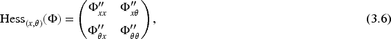
A smooth function $Φ : (x, θ) \mapsto Φ (x, θ)$ , $θ \in R^{N}$ , defined near $(x_{0}, θ_{0})$ with $ξ_{0} = \partial_{x} Φ (x_{0}, θ_{0})$ is called a non-degenerate phase function in the sense of Hörmander iff the $(n + N) \times N$ matrix $(Φ_{θ x}^{″}, Φ_{θ θ}^{″})$ has rank $N$ on the critical set

\begin{aligned} C_{Φ} = {(x, θ) \in M \times R^{N} : \frac{\partial Φ}{\partial θ} (x, θ) = 0} . \end{aligned}

(3.2)

Then

\begin{aligned} ι_{Φ} : C_{Φ} \to Λ_{Φ} = {(x, Φ_{x}^{'} (x, θ) : (x, θ) \in C_{Φ}}, \end{aligned}

(3.3)

is a local Lagrangian embedding (diffeomorphism).

It is easy to prove (Ivrii, 1998), (1.2.7) that

\begin{aligned} N - rank Φ_{θ θ}^{″} = n - rank d π_{Λ} (ι_{Φ} (x, θ)) . \end{aligned}

(3.4)

Let also

π_{Λ_{Φ}} : Λ_{Φ} \to M

(or simply

π_{x}

) be the natural projection. If

k = rank d π_{Λ} (ι_{Φ} (x_{0}, θ_{0}))

, we say that

Λ_{Φ}

has rank

k

in a neighborhood

U

(x_{0}, ξ_{0})

, and call

U

a local chart of rank

(\geq) k

near

(x_{0}, ξ_{0})

. If

k = n

U

is called a “regular” chart, and

Λ_{Φ}

is called “projectable” or “horizontal” on

U

. On the other extreme, if

k = 0

U

is called a “maximally singular” chart, and

Λ_{Φ}

is called “vertical” on

U

If at some $z = (x, ξ) \in T^{*} M$ , $T_{z} Λ_{Φ}$ is transverse to the vertical plane $V_{z} = {(0, δ ξ)}$ (i.e., $z$ is a regular point) then equation (3.4) shows that $Φ_{θ θ}^{″}$ is of the maximal rank $N$ .

When $k < n$ we start to add some extra variables: namely there exists a partition of variables $x = (x^{'}, x^{″})$ such that the $(N + n - k) \times (N + n - k)$ matrix

\begin{aligned} {Hess}_{(x^{″}, θ)} (Φ) = (\begin{matrix} Φ_{x^{″} x^{″}}^{″} & Φ_{x^{″} θ}^{″} \\ Φ_{θ x^{″}}^{″} & Φ_{θ θ}^{″} \end{matrix}) \end{aligned}

(3.5)

is non-degenerate. So the map

(x^{″}, θ) \mapsto Φ (x, θ) - x^{″} ξ^{″}

has a non-degenerate critical point

θ_{c} = θ (x^{'}, ξ^{″}), x_{c}^{″} = x^{″} (x^{'}, ξ^{″})

with the critical value

S (x^{'}, ξ^{″}) = Φ (x^{'}, x_{c}^{″}, θ) - x^{'} ξ_{c}^{″}

. The projection

\tilde{π} : Λ_{Φ} \to T_{x}^{*} R^{n}, (x, ξ) \mapsto \tilde{π} (x, ξ) = (x^{'}, ξ^{″})

becomes of maximal rank

n

. Hence

Λ_{Φ}

near

x

is parametrized by

S (x^{'}, ξ^{″})

Remark 3.1

The above non-degeneracy condition on $Φ$ is equivalent to (non-degeneracy in the sense of Hörmander) $d_{x, θ} Φ (x_{0}, θ_{0}) \neq 0$ , and $d_{(x, θ)} \partial_{θ_{1}} Φ, \dots, d_{(x, θ)} \partial_{θ_{N}} Φ$ are linearly independent on the critical set $C_{Φ}$ . The property stated above means that, if $Φ$ is non-degenerate in the sense of Hörmander, then it is always possible to find coordinates such that $π_{ξ} : (x, ξ) \mapsto ξ$ has rank $n$ . Actually, there are coordinates such that $(x, θ) \mapsto Φ (x, θ) - x ξ$ has a non-degenerate critical point, so that

\begin{aligned} {Hess}_{(x, θ)} (Φ) = (\begin{matrix} Φ_{x x}^{″} & Φ_{x θ}^{″} \\ Φ_{θ x}^{″} & Φ_{θ θ}^{″} \end{matrix}), \end{aligned}

(3.6)

is non-degenerate and

Λ_{Φ}

is of the form

Λ_{Φ} = {(- ϕ^{'} (ξ), ξ)}

(see Hörmander, 2009, Proposition 25.1.5). This follows from the fact that while

π_{x} : (x, ξ) \mapsto x

is invariantly defined under diffeomorphisms in

M

, this is not the case for the horizontal projection

π_{ξ} : (x, ξ) \mapsto ξ

. For the generating function

Φ

Λ_{+}^{E}

constructed in Section 4 below,

{Hess}_{(x, θ)} (Φ)

is actually degenerate in the “natural” coordinates of the problem, while

{Hess}_{(x^{″}, θ)} (Φ)

is not, see Remark 4.4.

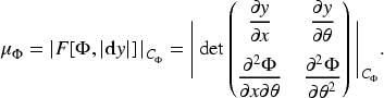
Let us recall the expression for the (inverse) density on $C_{Φ}$ . Let $y = (y_{1}, \dots, y_{n})$ be some local coordinates on $C_{Φ}$ and $| d y |$ corresponding Lebesgue measure. Then the non-vanishing, real function

\begin{aligned} F [Φ, | d y |] = \frac{d y \land d Φ_{θ}^{'}}{d x \land d θ} = \frac{d y \land d Φ_{θ_{1}}^{'} \land \dots \land d Φ_{θ_{N}}^{'}}{d x \land d θ_{1} \land \dots \land d θ_{N}} \end{aligned}

(3.7)

is well-defined near

C_{Φ}

as the quotient of two volume forms, see Hörmander (2009), Vol.IV, p.14, Dobrokhotov et al. (2017), (2.8), and Anikin et al. (2023). Restricted to

C_{Φ}

, its absolute value

μ_{Φ}

defines the (inverse) density on

C_{Φ}

. Computed on the complexified tangent space to

C_{Φ}

, the variations of the argument of

F [Φ]

can define also the variations of Maslov index (see Anikin et al., 2023; Dobrokhotov et al., 2017), which we shall ignore in this article. We can also write the absolute value of (3.7) on

C_{Φ}

in the form (see Grigis & Sjöstrand, 1994, Section 11)

\begin{aligned} μ_{Φ} = | F [Φ, | d y |] |_{C_{Φ}} = | det (\begin{matrix} \frac{\partial y}{\partial x} & \frac{\partial y}{\partial θ} \\ \frac{\partial^{2} Φ}{\partial x \partial θ} & \frac{\partial^{2} Φ}{\partial θ^{2}} \end{matrix}) |_{C_{Φ}} . \end{aligned}

It is actually independent of the choice of coordinates on

C_{Φ}

but it does depend on the choice of local coordinates

x

3.2. Maslov Canonical Operator Acting on Lagrangian Distributions

Let $u_{h}$ be a semi-classical Lagrangian distribution (or oscillatory integral), that is, locally

\begin{aligned} u_{h} (x) = \int^{*} e^{i Φ (x, θ) / h} b (x, θ; h) d θ, \end{aligned}

(3.8)

where

Φ (x, θ)

is a non-degenerate phase function in the sense above, and

b (x, θ; h) = b_{0} (x, θ) + h b_{1} (x, θ) + \dots

an amplitude. With

u_{h}

we associate as in (3.3) the Lagrangian submanifold

Λ_{Φ}

It is proved by Hörmander (2009, Proposition 25.1.5) that, using that (3.6) is non-degenerate, we can choose local coordinates $ξ \in R^{n}$ on $Λ_{Φ}$ , take $h$ -Fourier transform $F_{h, x \to ξ} u_{h} (ξ) = (2 π h)^{- n / 2} \int e^{- i x ξ / h} u (x) d x$ and expand by the stationary phase. The half-density in the local chart $(C_{Φ}, ι_{Φ})$ is the given by $\sqrt{d μ_{Φ}} = | det Φ^{″} |^{- 1 / 2} | d ξ |^{1 / 2}$ (denoting $Φ^{″} = {Hess}_{(x, θ)} (Φ)$ for short), and the (oscillating) principal symbol of $u_{h}$ in $Λ_{Φ}$ by

\begin{aligned} e^{i ϕ (ξ) / h} A_{0} (ξ) = e^{i ϕ (ξ) / h} e^{i π sgn Φ^{″} / 4} b_{0} (x (ξ), θ (ξ)) \sqrt{d μ_{Φ}} . \end{aligned}

(3.9)

Here

ϕ

is the “reduced phase function” such that

Λ_{Φ} = {(- ϕ^{'} (ξ), ξ)}

. We emphasize that the factor

e^{i ϕ (ξ) / h}

in (3.9) is due to the fact that the Lagrangian manifold

Λ_{Φ}

is not necessarily conic in

ξ

(see e.g., Duistermaat, 1974, p. 222).

Alternatively, when (3.5) is non-degenerate, one can express the (oscillating) principal symbol of $u_{h}$ taking partial Fourier transform

\begin{aligned} v_{h} (x^{'}, ξ^{″}; h) = F_{h, x^{″} \to ξ^{″}} u_{h} (x^{'}, ξ^{″}) = (2 π h)^{(k - n) / 2} \int e^{- i x^{″} ξ^{″} / h} d x^{″} \int e^{i Φ (x^{'}, x^{″}, θ) / h} b (x^{'}, x^{″}, θ; h) d θ, \end{aligned}

leading again to an expression of WKB type as in (3.9), and locally

\begin{aligned} Λ_{Φ} = Λ_{S} = {(x, ξ) : x^{″} = - \partial_{ξ^{″}} S (x^{'}, ξ^{″}), ξ^{'} = \partial_{x^{'}} S (x^{'}, ξ^{″})} . \end{aligned}

Thus we obtained a reduced phase functions, with least possible number of variables

θ

, that is, at most

n

. When

k = n

, then

u_{h}

assumes simply a WKB form in

x

variables.

Conversely, let $ι : L \to T^{*} M$ be a Lagrangian immersion. We know (Hörmander, 2009, Theorem 21.2.16) that there exists a covering of $L$ by canonical charts $U$ , such that $L$ is parametrized in each $U$ by a non-degenerate phase function $Φ$ . The Lagrangian immersions $ι$ and (3.3) have the same image on $U$ and $C_{Φ}$ is a submanifold of dimension $n$ . In particular, $ι_{Φ} : C_{Φ} \to L$ is a diffeomorphism onto its image. These phases can be chosen coherently, and define a class of “reduced phase functions” $ϕ$ , parametrizing $ι$ locally. This gives the fiber bundle of phases $L_{h}$ , including Maslov indices, equipped with transition functions. We are also given local smooth half-densities $| d μ_{Φ} |^{1 / 2}$ on $L$ , defining the fiber bundle of half-densities $Ω^{1 / 2}$ , equipped with transition functions. The collection of these objects make a fiber bundle $Ω^{1 / 2} \otimes L_{h}$ over $L$ . A section of $Ω^{1 / 2} \otimes L_{h}$ will be written as $[K_{(L, μ)}^{h} a] (x; h)$ , where $K_{(L, μ)}^{h}$ is called Maslov canonical operator. At leading order $[K_{(L, μ)}^{h} a]$ reduces to its oscillating symbol (3.9). The set of such Lagrangian distributions microlocally supported on $L$ will be denoted by $I (M; L)$ .

We apply Maslov canonical operator for constructing solutions to homogeneous equation

\begin{aligned} (H (x, h D_{x}; h) - E) u_{h} = 0, \end{aligned}

microlocally supported on

L = Λ_{+}^{E}

in the characteristic foliation of

Σ_{E}

. Here

H (x, h D_{x}; h)

is a

h

-PDO with principal symbol

H (x, p)

, and we assume for short

E = 0

, so that we denote

Λ_{+}^{E}

Λ_{+}^{0}

. If

u_{h}

is a Lagrangian distribution locally of the form (3.8), then the same holds for

H u_{h}

The phase $Ψ$ (with time $t$ in Hamilton equations as one of the $θ$ -parameters) is determined by the HJ equation (2.10), with the initial data on $t = 0$ , which gives (locally) the Lagrangian embedding (3.3) with image $Λ_{+}$ . Alternatively, we can use the 1-jet $Φ$ of $Ψ$ along $Λ_{+}^{0}$ as above. In particular, $C_{Φ} \subset {\partial_{t} Φ = 0}$ . We prescribe the amplitude such that $b |_{t = 0} = a$ . The construction of $[K_{(Λ_{+}^{0}, μ)}^{h} a]$ goes as follows. The amplitude of $H (x, h D_{x}; h) u_{h} (x)$ has leading term

\begin{aligned} H_{0} (x, \partial_{x} Φ (x, θ)) b_{0} (x, θ) . \end{aligned}

Moreover, if

H (x, p; h)

has sub-principal symbol

H_{1} (x, p)

, and

H_{0} (x, p) = 0

Λ_{+}^{0}

H (x, h D_{x}; h) u_{h} (x)

has principal symbol

\begin{aligned} h (\frac{1}{i} L_{v_{H_{0}}} |_{Λ_{+}} + H_{1}) b_{0} | d μ_{Φ} |^{1 / 2}, \end{aligned}

(3.10)

where

L_{v_{H_{0}}}

denotes the Lie derivative along

v_{H_{0}}

acting on half-densities

u | d y |^{1 / 2}

as follows:

\begin{aligned} L_{v} (u | d y |^{1 / 2}) = (\sum_{j} v_{j} (y) \frac{\partial u}{\partial y_{j}} + \frac{1}{2} (div v (y)) u (y)) | d y |^{1 / 2}, \end{aligned}

(3.11)

in local coordinates. For Schrödinger operator

H (x, h D_{x}) = - h^{2} Δ + V (x)

Λ_{+}

is “horizontal,” and

L_{v_{H_{0}}} |_{Λ_{+}} (b_{0} | d μ_{Φ} |^{1 / 2})

takes the form

(\sum_{j} Φ_{j}^{'} (x) \frac{\partial b_{0}}{\partial x_{j}} + \frac{1}{2} Δ Φ (x) b_{0} (x)) | d x |^{1 / 2}

, and a similar expression when

Λ_{+}

is “vertical,” (see e.g., Dobrokhotov & Rouleux, 2011, b. 14). Then (3.9) solves

H u_{h} = 0

mod

O (h^{2})

Note that on $Λ_{+}$ , $L_{v_{H_{0}}} = d / d t$ . Provided $Φ$ is a non-degenerate phase-function, (3.10) admits a global solution, computed on each canonical chart. For instance, on a regular chart, this is just WKB construction. In a totally singular chart instead, we solve (3.10) in Fourier representation, and more generally in the mixed representation.

The function $b_{0} (x (ξ), θ (ξ))$ is smooth in $ξ$ , but of course when expressed in $x$ -variable, singularities may occur due to singular Jacobians at focal points.

The fact that $u_{h}$ solves $H u_{h} = 0$ mod $O (h^{2})$ is also expressed by the commutation relation

\begin{aligned} H (x, h D_{x}; h) [K_{(Λ_{+}, μ)}^{h} a] (x; h) = [K_{(Λ_{+}, μ)}^{h} h (\frac{d b_{0}}{d t} + i H_{1} b_{0})] (x; h) + O (h^{2}) = O (h^{2}) . \end{aligned}

(3.12)

3.3. Bi-Lagrangian Distributions

According to Melrose and Uhlmann (1979), see also Han, our constructions make use of symbolic calculus adapted to Lagrangian intersection. So we need first to translate some notions relative to asymptotics with respect to smoothness (or “standard Pseudo-differential Calculus”), to the framework of asymptotics with respect to small parameter $h$ (or “ $h$ -Pseudo-differential Calculus”), in particular to allow for general phase functions, without homogeneity in the momentum variable. We need also to keep track of the energy parameter.

Let $ι_{0} : Λ_{0} \to T^{*} M$ be a smooth embedded Lagrangian manifold, and $ι_{1} : Λ_{1} \to T^{*} M$ be a smooth embedded Lagrangian manifold with smooth boundary $\partial Λ_{1}$ (isotropic manifold). Following Melrose and Uhlmann (1979), we say that $(Λ_{0}, Λ_{1})$ is an intersecting pair of Lagrangian manifolds iff $Λ_{0} \cap Λ_{1} = \partial Λ_{1}$ and the intersection is clean, that is,

\begin{aligned} \forall z \in \partial Λ_{1} T_{z} Λ_{0} \cap T_{z} Λ_{1} = T_{z} \partial Λ_{1} . \end{aligned}

On the set of intersecting pairs of Lagrangian manifolds we define an equivalence relation by saying that

(Λ_{0}, Λ_{1}) \sim (L_{0}, L_{1})

iff near any

z \in \partial Λ_{1}

z^{'} \in \partial L_{1}

, there is a symplectic map

κ

such that

κ (z) = z^{'}

, and a neighborhood

V \subset T^{*} M

z

such that

κ (Λ_{0} \cap V) \subset L_{0}

κ (Λ_{1} \cap V) \subset L_{1}

. We will call the equivalence class a Lagrangian pair.

All intersecting pairs of manifolds in $T^{*} M$ are locally equivalent. This results from Darboux theorem see, for example, Hörmander (2009, Volume 3), or Grigis and Sjöstrand (1994) suitably adapted to a pair of Lagrangian manifolds with non-glancing intersection by Melrose and Uhlmann (1979, Proposition 1.3). The following proposition extends (Melrose & Uhlmann, 1979, Proposition 1.3) in the case of homogeneous Lagrangian manifolds:

Proposition 3.2
Let $(Λ_{0}, Λ_{1})$ be an intersecting pair, and $z \in Λ_{0} \cap Λ_{1}$ . Then there exists a neighborhood $V \subset T^{} M$ of $z$ , and a canonical map $κ : T^{} M \to T^{} R^{n}$ such that $κ (z) = (0, 0)$ , $κ (Λ_{0} \cap V) \subset T_{0}^{} R^{n}$ (vertical fiber at 0), and $κ (Λ_{1} \cap V) \subset L_{+}^{0}$ , $L_{+}^{0}$ as in (1.10) being the flow-out of $T_{0}^{} R^{n}$ by the Hamilton vector field $v_{ξ_{n}} = ((0, \dots, 0, 1), 0)$ of $ξ_{n}$ , passing through some $(0; ξ) = (0; (ξ^{'}, 0))$ , that is,
$\begin{aligned} L_{+}^{0} = {(x, ξ) \in T^{} R^{n} : x = (0, x_{n}), ξ = (ξ^{'}, 0), x_{n} > 0}, \end{aligned}$
(3.13)
(superscript 0 is relative to the energy level).

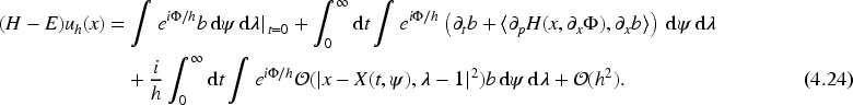
So this pair of Lagrangian manifolds is in the class of intersecting pairs, that is, in some local canonical charts $Λ_{0} = L_{+}^{0}$ and $H (x, p) = E + p_{n}$ . In particular, $(Λ_{0}, Λ_{+}^{E})$ are mapped onto $(L_{0}, L_{+}^{0})$ by a canonical transformation sending $\partial Λ_{+}^{E} = Λ_{0} \cap Λ_{+}^{E}$ onto $\partial L_{+}^{0} = L_{0} \cap L_{+}^{0}$ .

As a warm-up, let us construct $u_{h} = E_{+} (h) f_{h}$ mod $O (h^{\infty})$ for $h D_{x_{n}}$ , and $f_{h}$ as in (1.2) with $a$ compactly supported. By a gauge transformation and a shift of the support of $ξ_{n} \mapsto a (x, ξ)$ in (1.2), we may assume $E = 0$ . So, we just need to compute a primitive of $f_{h} (x)$ . Hamilton equations give in this case $X (t) = (X^{'} (t), X_{n} (t)) = (0, t)$ and $z (t) = (X (t), (ξ^{'}, 0))$ , so in particular $| z (t) | \to \infty$ as $t \to + \infty$ . Let $T > 0$ and $θ_{T} \in C^{\infty} (R_{+})$ vanishing near $+ \infty$ and $θ_{T} (t) = 1$ for $t \leq T$ . We consider
$\begin{aligned} u_{h} (x) = \frac{i}{h} \int_{0}^{\infty} θ_{T} (t) d t \int^{} e^{i (x^{'} ξ^{'} + (x_{n} - t) ξ_{n}) / h} a (x^{'}, x_{n} - t, ξ; h) d ξ . \end{aligned}$
(3.14)
Provided $x_{n} \leq T / 2$ (say) integration by parts and a non-stationary phase argument in variables $(t, ξ_{n})$ show that
$\begin{aligned} h D_{x_{n}} u_{h} (x) = f_{h} (x) + O (h^{\infty}) . \end{aligned}$
(3.15)
Note that by Hörmander (2009, Lemma 18.2.1) we could already assume $a = a (ξ; h)$ . This will be crucial for the compatibility condition* (see below).

We need to adapt to the semi-classical case the symbolic calculus considered by Melrose and Uhlmann (1979).

To this end, we need to generalize (3.14), including local semi-classical distributions of the form
$\begin{aligned} u_{h} (x) = \frac{i}{h} \int_{0}^{\infty} θ_{T} (t) d t \int^{} e^{i (x^{'} ξ^{'} + (x_{n} - t) ξ_{n}) / h} b (t, x, ξ; h) d ξ, \end{aligned}$
(3.16)
where $b$ is an amplitude, and $θ_{T} (t)$ a cut-off as in (3.14), which we omit for simplicity, since our analysis is local in $x$ .

Let us first compute the semi-classical wave-front set ${WF}_{h} u_{h}$ in (3.16). Fix $\bar{z} = (\bar{x}, \bar{ξ}) \in T^{} M$ , $\bar{ξ} = ({\bar{ξ}}^{'}, {\bar{ξ}}_{n})$ . It is well-known that ${WF}_{h} (u_{h})$ is characterized by the following property: $\bar{z} \notin {WF}_{h} (u_{h})$ iff there exists $χ \in C_{0}^{\infty} (T^{} M)$ equal to 1 near $\bar{z}$ , such that
$\begin{aligned} χ (x, h D_{x}) u_{h} (x) = (2 π h)^{- 1} \int \int e^{i (x - y) η / h} χ (y, η) u_{h} (y) d y d η = O (h^{\infty}) . \end{aligned}$
(3.17)
We have the standard
Proposition 3.3
Let $u_{h}$ be as in (3.16). Then
$\begin{aligned} {WF}_{h} (u_{h}) \subset {x_{n} \geq 0} \cap ({x_{n} = 0} \cup {x^{'} = 0} \cup {ξ_{n} = 0}) . \end{aligned}$
(3.18)
If moreover $b (t, x, ξ; h)$ verifies the transport equation $\partial_{t} b + \partial_{x_{n}} b = 0$ , we get the sharper estimate ${WF}_{h} (u_{h}) \subset Λ_{0} \cup Λ_{+}^{0}$ , $Λ_{0} = T_{0}^{} R^{n}$ , which is the conormal bundle of the manifold with boundary $x^{'} = 0, x_{n} \geq 0$ . Here we recall from Proposition 3.2 that $Λ_{+}^{0} \subset Char h D_{x_{n}}$ is the flow out of $Λ_{0}$ by $v_{ξ_{n}}$ in $ξ_{n} = 0$ .
Proof.
Since we work locally in $x$ , we can safely omit the cut-off $θ_{T}$ in (3.16). Let $Φ_{t} (x, ξ, y, η) = y^{'} ξ^{'} + (y_{n} - t) ξ_{n} + (x - y) η$ be the phase-function in (3.16). (i)
If ${\bar{x}}_{n} < 0$ , we choose $χ$ such that $χ (y, η) = \tilde{χ} (y^{'}, η) χ_{n} (y_{n})$ , with $χ_{n} ({\bar{x}}_{n}) \neq 0$ . It follows that $η_{n} \mapsto Φ_{t}$ is non-stationary in $supp χ_{n}$ , so ${WF}_{h} u_{h} \subset {x_{n} \geq 0}$ .
(ii)
Assume ${\bar{ξ}}_{n} \neq 0$ and choose $χ$ such that $χ = \tilde{χ} (y, η^{'}) χ_{2 n} (η_{n})$ , with $χ_{2 n} ({\bar{ξ}}_{n}) \neq 0$ . Let $ε$ be so small that $| ξ_{n} - η_{n} | > δ > 0$ on $| ξ_{n} | < ε$ and $η_{n} \in supp χ_{2 n}$ , we split $χ$ according to $χ^{ε}$ and ${\hat{χ}}^{ε} = χ - χ^{ε}$ , where $χ^{ε} (x, h D_{x}) u_{h} (x) = (2 π h)^{- n} \int d y \int_{| ξ_{n} | \geq ε} \int e^{i (x - y) η / h} χ (y, η) u_{h} (y) d η$ .

We have $h D_{t} e^{i Φ_{t} / h} = - ξ_{n} e^{i Φ_{t} / h}$ , so that integrating by parts $N$ times with respect to $t$ we get $χ^{ε} (x, h D_{x}) u_{h} (x) = (\frac{h}{i})^{N} A_{N}^{ε} (x; h) + B_{N}^{ε} (x; h)$ , where
$\begin{aligned} A_{N}^{ε} (x; h) & = (2 π h)^{- n} \int χ (y, η) d y d η \int_{0}^{\infty} d t \int_{| ξ_{n} | \geq ε}^{} e^{i Φ_{t} / h} \frac{1}{ξ_{n}^{n + 1}} \partial_{t}^{N + 1} b (t, y, ξ; h) d ξ, \\ B_{N}^{ε} (x; h) & = (2 π h)^{- n} \int χ (y, η) d y d η \int_{| ξ_{n} | \geq ε}^{} e^{i Φ_{0} / h} \frac{1}{ξ_{n}} \sum_{j = 0}^{N} {(\frac{h}{i ξ_{n}})}^{j} \partial_{t}^{j} b (0, y, ξ; h) d ξ . \end{aligned}$
(3.19)
Now $(y, ξ) \mapsto Φ_{0} (x, ξ, y, η) = y ξ + (x - y) η$ has a non-degenerate critical point at $ξ = η, y = 0$ . Assume $\bar{x} \neq 0$ , that is, we choose $χ$ such that $0 \notin π_{x} (supp χ)$ ; so $Φ_{0}$ is not stationary and $B_{N}^{ε} (x; h) = O (h^{\infty})$ . Hence $χ^{ε} (x, h D_{x}) u_{h} (x) = O (h^{N})$ for any $N$ .

Consider next the contribution ${\hat{χ}}^{ε} (x, h D_{x}) u_{h} (x)$ of $| ξ_{n} | < ε$ to $χ (x, h D_{x}) u_{h} (x)$ . The map
$\begin{aligned} y_{n} \mapsto Φ_{t} (x, ξ, y, η), \end{aligned}$
has a critical point at $ξ_{n} = η_{n}$ . Since $| ξ_{n} - η_{n} | > δ > 0$ when $η_{n} \in supp χ_{2 n}$ , $y_{n} \mapsto Φ_{t} (x, ξ, y, η)$ is non-stationary and ${\hat{χ}}^{ε} u_{h} (x) = O (h^{\infty})$ . Altogether, $χ (x, h D_{x}) u_{h} (x) = χ^{ε} u_{h} (x) + {\hat{χ}}^{ε} u_{h} (x) = O (h^{\infty})$ so $\bar{z} \notin {WF}_{h} u_{h}$ if ${\bar{ξ}}_{n} \neq 0$ . In particular, ${WF}_{h} u_{h} \subset {x_{n} \geq 0} \cap ({ξ_{n} = 0} \cup {x = 0})$ .
(iii)
Assume next ${\bar{x}}_{n} > 0$ and take as above $χ (y, η) = \tilde{χ} (y^{'}, η) χ_{n} (y_{n})$ , with $χ_{n} ({\bar{x}}_{n}) \neq 0$ . Then $(t, ξ_{n}, y, η) \mapsto Φ_{t}$ is critical at $t = y_{n} = x_{n}, ξ_{n} = 0, y^{'} = x^{'}, η^{'} = x^{'}$ , and this is a non-degenerate critical point. So when $x_{n} > 0$ , asymptotic stationary phase (3.1) shows that
$\begin{aligned} χ (x, h D_{x}) u_{h} (x) = 2 i π \int^{} e^{i x^{'} ξ^{'} / h} \tilde{χ} (x^{'}, ξ^{'}) [b (x_{n}, x, (ξ^{'}, 0); h) + \frac{h}{i} \frac{\partial^{2} b_{0}}{\partial t \partial ξ_{n}} (x_{n}, x, (ξ^{'}, 0))] d ξ^{'} . \end{aligned}$
(3.20)
In particular, using (i), we see that ${WF}_{h} (u_{h}) \subset {x_{n} \geq 0} \cap ({x_{n} = 0} \cup {x^{'} = 0})$ , which altogether proves (3.17).

For the last statement of Proposition 3.3, apply $h D_{x_{n}}$ to $u_{h}$ and integrate (3.16) by parts once with respect to $t$ . We find
$\begin{aligned} h D_{x_{n}} u_{h} (x) = \int^{} e^{i x ξ / h} b (0, x, ξ; h) d ξ + \int_{0}^{\infty} d t \int^{} e^{i Φ_{t} / h} (\partial_{t} + \partial_{x_{n}}) b (t, x, ξ; h) d ξ, \end{aligned}$
(3.21)
so if $b (t, x, ξ; h)$ verifies the transport equation, $h D_{x_{n}} u_{h} (x) = g_{h} (x) = \int^{} e^{i x ξ / h} b (0, x, ξ; h) d ξ$ and since ${WF}_{h} g_{h} \subset T_{0}^{} R^{n}$ , the last (sharper) estimate on ${WF}_{h} u_{h}$ follows from the well-known property ${WF}_{h} u_{h} \subset {WF}_{h} h D_{x_{n}} u_{h} \cup Char h D_{x_{n}}$ .□

Then, we must show that a $h$ -FIO $A$ “quantizing” the canonical transformation in Proposition 3.2, that is, whose canonical map preserves the Lagrangian intersection, preserves also bi-Lagrangian distributions of the form (3.16). Namely, let $(L, L_{+}) \sim (Λ, Λ_{+})$ be Lagrangian pairs in the sense of Proposition 3.2, $(y_{0}, η_{0}) \in \partial L_{+}$ , and $u_{h}$ be of the form (3.16). Proposition 3.2 of Melrose & Uhlmann (1979) readily extends as follows:

Proposition 3.4
Let $(L, L_{+}) \sim (Λ, Λ_{+})$ be Lagrangian pairs in the sense of Proposition 3.2. Let $A$ be a $h$ -FIO of the form
$\begin{aligned} A v (x; h) = (2 π h)^{- (n + N) / 2} \int e^{i ϕ (x, y, θ) / h} c (x, y, θ) v (y; h) d y d θ, \end{aligned}$
associated with the canonical transformation $κ_{A}$ , $κ_{A} (y_{0}, η_{0}) = (x_{0}, ξ_{0})$ with graph
$\begin{aligned} Λ_{A} = {(x, ϕ_{x}^{'} (x, y, θ), y; ϕ_{y}^{'} (x, y, θ) : ϕ_{θ}^{'} (x, y, θ) = 0}, \end{aligned}$
such that (locally) $Λ_{A} \circ L = Λ$ , $Λ_{A} \circ L_{+} = Λ_{+}$ and the compositions are transversal Hörmander (2009), Vol. IV, p.19 and 44. Here have denoted as usual $Λ_{A}^{'} = {(x, ξ; y, - η) : (x, ξ; y, η) \in Λ_{A}}$ . Let $u_{h}$ be defined near $(y_{0}, η_{0})$ on the Lagrangian pair $(L, L_{+})$ by (3.16). Then $A u_{h}$ defined near $(x_{0}, ξ_{0})$ on the Lagrangian pair $(Λ, Λ_{+})$ is again of the form (3.16).

The proof essentially reduces to show that $A u_{h}$ , after a change of $(t, θ)$ variables, can be rewritten as an integral of the form (3.16), that is, with the same phase $Φ_{t}$ , and a new amplitude $b^{'} (t, x, ξ; h)$ .

So we can define the class $I (M, Λ, Λ_{+})$ of bi-Lagrangian distributions supported on the Lagrangian pair $(Λ, Λ_{+}) \sim (L, L_{+})$ , all of which take locally the form (3.16).

We say that $u_{h} \in I (M, Λ, Λ_{+})$ is a bi-Lagrangian* (semi-classical) distribution on the intersecting pair $(Λ, Λ_{+})$ .

Consider now the inhomogeneous equation $H (x, h D_{x}; h) u_{h} = f_{h}$ , where
$\begin{aligned} f_{h} (x) = \int^{} e^{i x ξ / h} a (x, ξ; h) d ξ, \end{aligned}$
is conormal to $Λ = Λ_{0} = T_{0}^{} M$ .

When $H (x, h D_{x}; h) = h D_{x_{n}}$ , $u_{h}$ solves $H (x, h D_{x}; h) u_{h} = f_{h}$ whenever $b$ solves the transport equation, that is, $b (t, x, ξ; h) = a (x^{'}, x_{n} - t, ξ; h)$ , so that (3.21) simplifies to $h D_{x_{n}} u_{h} (x) = f_{h} (x)$ mod $O (h^{\infty})$ .

In the general case, we can show that we can take $H (x, h D_{x};)$ to its normal form $h D_{y_{n}}$ by conjugating with a suitable $h$ -FIO as in Proposition 3.4. Namely, we have the following proposition.
Proposition 3.5
Let the energy surface $H_{0} = E$ be non-critical, and $v_{H_{0}}$ be transverse to $Λ$ at $(x_{0}, ξ_{0}) \in \partial Λ_{+}$ , where $Λ_{+}$ is the flow out of $v_{H}$ from $Λ$ . Then there is a $h$ -FIO $A$ , as in Proposition 3.4, defined microlocally near $((x_{0}, ξ_{0}), (0, 0))$ , quantizing the canonical transformation of Proposition 3.2 such that $A^{- 1} H (x, h D_{x}) A = h D_{y_{n}}$ .

We could presumably take $A$ (microlocally) unitary as in the case without a boundary, but this will not be needed.
3.4. Compatibility Condition and Symbolic Calculus. Maslov Canonical Operator for Bi-Lagrangian Disributions

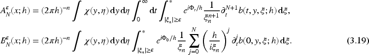
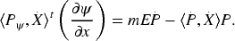
Now we prove Theorem 1.1. By Propositions 3.4 and 3.5, it suffices to consider the Lagrangian pair $(Λ^{0}, Λ_{+}^{0})$ , with $Λ^{0} = T_{0}^{*} R^{n}$ (which we denote again $Λ$ for short). When $u_{h}$ solves $(H (x, h D_{x}; h) - E) u_{h} (x) = f_{h}$ mod $O (h^{N})$ we want to define the “boundary-part” $σ$ and “wave-part” $σ^{+}$ symbols of $u_{h}$ satisfying the compatibility condition (see also Melrose & Uhlmann, 1979, Section 4) for a more intrinsic discussion on $(σ, σ^{+})$ .

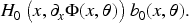
Our argument is similar to Melrose and Uhlmann (1979, Propostion 2.3), and relies on the fact that if $χ (x, h D_{x})$ is a $h$ -PDO with ${WF}_{h} (χ (x, h D_{x})) \cap Λ = {WF}_{h}^{'} (χ (x, h D_{x})) \circ Λ = \emptyset$ , then $χ (x, h D_{x}) u_{h}$ is a Lagrangian distribution supported on $Λ_{+}^{0}$ , while if $χ (x, h D_{x})$ is a $h$ -PDO with ${WF}_{h} (χ (x, h D_{x}) \cap Λ_{+}^{0} = \emptyset$ , then $χ (x, h D_{x}) u_{h}$ is a Lagrangian distribution supported on $Λ$ .

We proceed in two steps. In Step 1, we construct a family $(χ_{δ}^{+} (x, h D_{x}))_{δ > 0}$ such that $χ_{δ} (y, η) \to 1$ pointwise and $χ_{δ} (x, h D_{x}) u_{h}$ is supported on $Λ^{0}$ . This will give the boundary-part symbol. In Step 2, we construct a family $(χ_{δ} (x, h D_{x}))_{δ > 0}$ such that $χ_{δ}^{+} (y, η) \to 1$ pointwise and $χ_{δ}^{+} (x, h D_{x}) u_{h}$ is supported on $Λ_{+}^{0}$ . This will give the wave-part symbol. The compatibility condition results in comparing these two symbols.

$∙$ Step 1: The boundary-part symbol. We check first the compatibility condition for $N = 1$ . Consider $χ_{δ} \in C^{\infty} (R^{2 n})$ of the form $χ_{δ} (y, η) = χ_{δ}^{'} (y, η^{'}) χ_{2 n}^{δ} (η_{n})$ with $| η_{n} | \geq δ$ on $supp χ_{2 n}^{δ}$ , and $χ_{n}^{δ} (η_{n}) \to 1$ pointwise for $η_{n} \neq 0$ , as $δ \to 0$ . Let

\begin{aligned} q (y, ξ; h) = \frac{1}{ξ_{n}} [b (0, y, ξ; h) + \frac{h}{i ξ_{n}} \partial_{t} b_{0} (0, y, ξ) + O (h^{2})] . \end{aligned}

From part (ii) of the proof of Proposition 3.2 for

N = 1

, taking

ε < δ

so that the contribution of

| ξ_{n} | < ε

χ_{δ} (x, h D_{h}) u_{h} (x)

O (h^{\infty})

, we know that

\begin{aligned} χ_{δ} (x, h D_{x}) u_{h} (x) = B_{1}^{δ, ε} (x; h) + O (h^{2}) . \end{aligned}

(3.22)

We may assume

χ_{δ}

is such that

\partial χ_{δ} / \partial y (0, η) = 0

, hence computing

\begin{aligned} B_{1}^{δ, ε} (x; h) = \int e^{i x η / h} d η \int_{| ξ_{n} | > ε}^{*} e^{i y (ξ - η) / h} q (y, ξ; h) χ_{δ} (y, η) d y d ξ \end{aligned}

by asymptotic stationary phase in

(y, ξ)

with (3.1), where

A = A_{δ} = \partial^{2} Φ_{0} / \partial (y, ξ)^{2}

det A_{δ} = (- 1)^{n}

, gives

\begin{aligned} B_{1}^{δ, ε} (x; h) & = (det A_{δ})^{- 1 / 2} (2 i π h)^{n} \int d η e^{i x η / h} χ_{δ} (0, η) \\ \times [q (0, η; h) - \frac{h}{i η_{n}} \frac{\partial^{2} q_{0}}{\partial y^{'} \partial ξ^{'}} (0, 0, η) - \frac{h}{i η_{n}} \frac{\partial^{2} b_{0}}{\partial y_{n} \partial ξ_{n}} (0, 0, η) + \frac{h}{i η_{n}^{2}} \frac{\partial b_{0}}{\partial t} (0, 0, η) + O (h^{2})] \\ = (det A_{δ})^{- 1 / 2} (2 i π h)^{n} \int d η e^{i x η / h} χ_{δ} (0, η) \\ \times [\frac{1}{η_{n}} b (0, 0, η; h) + \frac{h}{i η_{n}^{2}} (\partial_{t} b_{0} (0, 0, η) + \partial_{y_{n}} b_{0} (0, 0, η)) - \frac{h}{i η_{n}} \frac{\partial^{2} b_{0}}{\partial y \partial ξ} (0, 0, η) + O (h^{2})] . \end{aligned}

(3.23)

The oscillating integral

u_{h}

solves

h D_{x_{n}} u_{h} = f_{h}

iff

b

satisfies the transport equation

\begin{aligned} \partial_{t} b (0, x, ξ; h) + \partial_{x_{n}} b (0, x, ξ; h) = 0, \end{aligned}

that is,

b (t, x, ξ; h) = b (x^{'}, x_{n} - t, ξ; h)

. Then (3.23) reduces to

\begin{aligned} B_{1}^{δ, ε} (x; h) = \int e^{i x η / h} χ_{δ} (0, η) \frac{1}{η_{n}} [b (0, 0, η; h) + i h \frac{\partial^{2} b_{0}}{\partial y \partial ξ} (0, 0, η)] d η + O (h^{2}), \end{aligned}

(3.24)

which makes sense since

| η_{n} | \geq δ

supp χ_{2 n}^{δ}

. So for

η_{n} \neq 0

we define the boundary symbol of

u_{h}

as follows:

\begin{aligned} σ (η; h) = \frac{1}{η_{n}} [b (0, 0, η; h) + i h \frac{\partial^{2} b_{0}}{\partial y \partial ξ} (0, 0, η)] . \end{aligned}

(3.25)

∙

Step 2: The wave-part symbol. Consider next

χ_{δ}^{+} \in C^{\infty} (R^{2 n})

of the form

χ_{δ}^{+} (y, η) = χ_{δ}^{' +} (y^{'}, η) χ_{n}^{δ} (y_{n})

with

y_{n} \geq δ

supp χ_{n}^{δ}

, and

χ_{n}^{δ} (η_{n}) \to 1

pointwise for

η_{n} > 0

, as

δ \to 0

. As in part (iii) in Proposition 3.2, we perform the integration

\begin{aligned} χ_{δ}^{+} (x, h D_{x}) u_{h} (x) = \frac{i}{h} \int_{0}^{\infty} d t \int χ_{δ}^{+} (y, η) d y d η \int^{*} e^{i Φ_{t} (x, ξ, y, η) / h} b (t, y, ξ; h) d ξ, \end{aligned}

by the asymptotic stationary phase (3.1) with respect to

(t, ξ_{n}, y, η)

. Here the Hessian is

A = A_{δ}^{+} = \partial^{2} Φ_{t} / \partial (t, ξ_{n}, y, η)^{2}

det A_{δ}^{+} = (- 1)^{n + 1}

, and the critical value of the phase is

Φ_{c} = x^{'} ξ^{'}

. We find

\begin{aligned} χ_{δ}^{+} (x, h D_{h}) u_{h} (x) & = \frac{i}{h} (det A_{δ}^{+})^{- 1 / 2} (2 i π h)^{n + 1} \int^{*} e^{i x^{'} ξ^{'} / h} χ_{δ}^{+} (x; ξ^{'}, 0) \\ \times [b (x_{n}, x, ξ^{'}, 0; h) - \frac{2 h}{i} \frac{\partial^{2} b_{0}}{\partial t \partial ξ_{n}} (x_{n}, x, ξ^{'}, 0)] d ξ^{'} + O (h^{2}) . \end{aligned}

(3.26)

So we define the wave-part symbol of

u_{h}

by letting

δ \to 0

as follows:

\begin{aligned} σ^{+} (ξ; h) = \frac{i}{h} (det A_{δ}^{+})^{- 1 / 2} (2 i π h)^{n + 1} [b (x_{n}, x, ξ^{'}, 0; h) - \frac{2 h}{i} \frac{\partial^{2} b_{0}}{\partial t \partial ξ_{n}} (x_{n}, x, ξ^{'}, 0)], \end{aligned}

(3.27)

and we are to compare (3.25) with (3.27).

From Hörmander (2009), Lemma 18.2.1 and its proof, we know that if $v_{h} (x) = \int e^{i x ξ / h} a (x, ξ; h) d ξ$ , then we also have $v_{h} (x) = \int e^{i x ξ / h} \tilde{a} (ξ; h) d ξ$ , with a symbol $\tilde{a} (ξ; h) \sim \sum_{j} h^{j} ⟨ - i D_{x}, D_{ξ} ⟩ a (x, ξ) / j!$ independent of $x$ . Applying this to amplitude $b (x^{'}, x_{n} - t, ξ)$ , the terms $\partial^{2} b_{0} / \partial y \partial ξ (0, 0, η)$ and $\partial^{2} b_{0} / \partial t \partial ξ_{n} (x_{n}, x, ξ^{'}, 0)$ respectively, in (3.24) and (3.26) disappear, $σ^{+} (ξ; h)$ is continuous up to $\partial Λ_{+}$ , and we end up with the compatibility condition (1.13) mod $O (h^{2})$ between the wave-part and boundary-part symbols on $\partial Λ_{+}$ .

It is clear, following again the proof of Proposition 3.2, that (3.22) carries by induction mod $O (h^{N})$ , all $N$ , when replacing $B_{1}^{δ, ε} (x; h)$ by $B_{N}^{δ, ε} (x; h)$ .

This allow to define coherently the (bi-)symbol $(σ, σ^{+}) = (σ (u_{h}), σ^{+} (u_{h}))$ computed as above in local coordinates, and thus by analogy with Section 3.2, an “effective” Maslov canonical operator $K_{Λ, Λ_{+}^{0}}^{h} (σ, σ^{+})$ . The commutation formula for bi-Lagrangian distributions takes the form

\begin{aligned} H (x, h D_{x}; h) [K_{Λ, Λ_{+}}^{h} (σ, σ^{+})] (x; h) & = [K_{Λ, Λ_{+}}^{h} ((H - E) σ, h (\frac{1}{i} L_{v_{H_{0}}} |_{Λ_{+}} + H_{1}) σ^{+}] (x; h) + O (h^{2}) \\ = f_{h} (x) + O (h^{2}), \end{aligned}

(3.28)

which gives (1.14) once the transport equation has been solved as in (3.10). This brings the proof of Theorem 1.1 to an end.

3.5. The Constant Coefficient Case

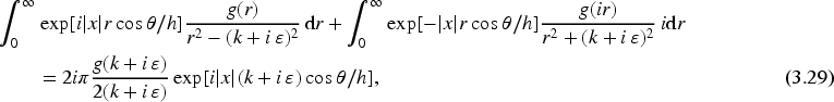
In general, it is difficult to obtain a decomposition of $u_{h}$ adapted to the splitting $u_{h} = u_{h}^{0} + u_{h}^{1}$ , where ${WF}_{h} (u_{h}^{0}) \subset Λ_{0}$ and ${WF}_{h} (u_{h}^{1}) \subset Λ_{+}^{E}$ .

Here, we compute $u_{h}$ explicitely in the 2D case for Helmholtz operator $- h^{2} Δ - E$ , but $f$ with compact support. Let $f$ also be radially symmetric; its Fourier transform $g = F_{1} f$ is again of the form $g (p) = g (| p |) = g (r)$ and extends holomorphically to $C^{2}$ . For $E = k^{2}$ , $k > 0$ , we rewrite as follows:

\begin{aligned} u_{h} (x) = (2 π h)^{- n} \int e^{i x ξ / h} \frac{F_{1} f (ξ)}{ξ^{2} - E - i 0} d ξ, \end{aligned}

u_{h} (x) = u (x) = u_{0} (x) + u_{1} (x)

with

\begin{aligned} u_{0} (x) & = \frac{k + i ε}{(2 π h)^{2}} \int_{0}^{2 π} d θ \int_{0}^{\infty} \exp [i | x | r \cos θ / h] \frac{g (r)}{r^{2} - (k + i ε)^{2}} d r, \\ u_{1} (x) & = \frac{1}{(2 π h)^{2}} \int_{0}^{2 π} d θ \int_{0}^{\infty} \exp [i | x | r \cos θ / h] \frac{g (r)}{r + k + i ε} d r . \end{aligned}

To compute

u_{0}

we use contour integrals. When

θ \in] - \frac{π}{2}, \frac{π}{2} [

, we shift the contour of integration to the positive imaginary axis and get by the residues formula

\begin{aligned} \int_{0}^{\infty} \exp [i | x | r \cos θ / h] \frac{g (r)}{r^{2} - (k + i ε)^{2}} d r + \int_{0}^{\infty} \exp [- | x | r \cos θ / h] \frac{g (i r)}{r^{2} + (k + i ε)^{2}} i d r \\ = 2 i π \frac{g (k + i ε)}{2 (k + i ε)} \exp [i | x | (k + i ε) \cos θ / h], \end{aligned}

(3.29)

while for

θ \in] \frac{π}{2}, \frac{3 π}{2} [

\begin{aligned} \int_{0}^{\infty} \exp [i | x | r \cos θ / h] \frac{g (r)}{r^{2} - (k + i ε)^{2}} d r - \int_{0}^{\infty} \exp [| x | r \cos θ / h] \frac{g (- i r)}{r^{2} + (k + i ε)^{2}} i d r = 0 . \end{aligned}

(3.30)

Summing up (3.29) and (3.30), integrating over

θ \in] 0, 2 π [

and letting

ε \to 0

, we obtain

\begin{aligned} u_{0} (x) & = \frac{i π g (k)}{(2 π h)^{2}} \int_{- π / 2}^{π / 2} \exp [i | x | k \cos θ / h] d θ \\ + \int_{0}^{\infty} \frac{d r}{r^{2} + k^{2}} [\int_{- π / 2}^{π / 2} g (i r) - \int_{π / 2}^{3 π / 2} g (- i r)] \exp [- | x | | \cos θ | / h] d θ . \end{aligned}

Since

g (i r) = g (- i r)

, the latter integral vanishes, so we end up with

\begin{aligned} u_{0} (x) = \frac{i π g (k)}{(2 π h)^{2}} \int_{- π / 2}^{π / 2} \exp [i | x | k \cos θ / h] d θ . \end{aligned}

It is readily seen that

\begin{aligned} {WF}_{h} u_{0} \subset {x = 0} \cup {(x, k \frac{x}{| x |}), x \neq 0} = Λ_{0} \cup Λ_{+}^{E} . \end{aligned}

Consider now

u_{1}

. We let

ε \to 0

and set

\tilde{g} (r) = g (r) / r (r + k)

. Since

\tilde{g} (r) \sqrt{r} \in L^{1} (R_{+})

, we have

u_{1} (x) = H_{0} (\tilde{g}) (| x | / h)

, where

H_{0}

denotes the Hankel transform of order 0. Let

χ \in C_{0}^{\infty} (R^{2})

be radially symmetric, and equal to 1 near 0, since

{WF}_{h} f_{h} = {x = 0}

, we have

\begin{aligned} g = F_{h} (χ f_{h}) + O (h^{\infty}) = (2 π h)^{- 2} F_{h} (χ) * g + O (h^{\infty}), \end{aligned}

so in the expression for

u_{1}

we may replace mod

O (h^{\infty})

\tilde{g} (r)

by a constant times

\hat{g} (r) = (F_{h} (χ) * g) (r) / r (r + m)

(see Baddour, 2009 for 2D convolution and Fourier transform in polar coordinates). To estimate

{WF}_{h} u_{1}

, we compute again the Fourier transform of

(1 - \tilde{χ}) \hat{g}

, where

\tilde{χ}

is a cut-off equal to 1 near 0, and we find it is again

O (h^{\infty})

χ \equiv 1

supp \tilde{χ}

. This shows that

{WF}_{h} u_{1} \subset {x = 0}

Note that this example makes use of Bessel function $J_{0} (| x | / h)$ , we shall return to such “localized functions” in Section 5.

f_{h}

is Supported Microlocally on the “Vertical Plane”

Here we shall construct objects written globally in a suitable coordinate system, using the phase functions in Section 2. This system consists only of coordinates on $Λ$ and of time parameter $t$ in Hamilton equations. This section relies in a strong way on Dobrokhotov et al. (2017).

Consider the case where $H_{0}$ is positively homogeneous of degree $m \geq 1$ with respect to $p$ and $f_{h}$ is microlocally concentrated on the vertical plane $Λ = {x = 0}$ , for example, $f_{h} (x) = h^{- n} f (x / h)$ , with $f \in S (R^{n})$ (Schwartz space).

4.1. Some Non-Degeneracy Condition

Recall first from Dobrokhotov et al. (2017, Lemma 6), the following result. Let $\tilde{ι} : \tilde{Λ} \to T^{*} \tilde{M}$ be a Lagrangian embedding of dimension $\tilde{n}$ , $U \subset \tilde{Λ}$ a connected simply connected open set,

\begin{aligned} (\tilde{ϕ}, \tilde{ψ}) = (ϕ_{1}, \dots, ϕ_{k}, ψ_{1}, \dots, ψ_{\tilde{n} - k}), \end{aligned}

local coordinates on

U

. Here the additional assumption of Dobrokhotov et al. (2017, Lemma 6) that

k

is the rank of

π_{x} : \tilde{Λ} \to \tilde{M}

, is not required. Thus

\tilde{Λ}

is defined by

x = X (\tilde{ϕ}, \tilde{ψ}), p = P (\tilde{ϕ}, \tilde{ψ})

in the chart

U

. Let

Π (\tilde{ϕ}, \tilde{ψ})

be a smooth

\tilde{n} \times k

matrix function defined in

U

such that:

\begin{aligned} Π^{*} (\tilde{ϕ}, \tilde{ψ}) X_{\tilde{ϕ}} (\tilde{ϕ}, \tilde{ψ}) = {Id}_{k \times k}, \\ κ : (\tilde{ϕ}, \tilde{ψ}) \mapsto (X (\tilde{ϕ}, \tilde{ψ}), \tilde{ψ}) is an embedding . \end{aligned}

(4.1)

Then there is a neighborhood

V

κ (U)

such that the system

\begin{aligned} Π^{*} (\tilde{ϕ}, \tilde{ψ}) (x - X (\tilde{ϕ}, \tilde{ψ})) = 0, (x, \tilde{ψ}) \in V, \end{aligned}

has a unique smooth solution

\tilde{ϕ} = \tilde{ϕ} (x, \tilde{ψ})

satisfying the condition

X (\tilde{ϕ} (x, \tilde{ψ}), \tilde{ψ}) = x

, when

(x, \tilde{ψ}) \in κ (U)

For $(\tilde{ϕ}, \tilde{ψ}) \in U$ , define the $\tilde{n} \times \tilde{n}$ matrix

\begin{aligned} M (\tilde{ϕ}, \tilde{ψ}) = (Π (\tilde{ϕ}, \tilde{ψ}); P_{\tilde{ψ}} (\tilde{ϕ}, \tilde{ψ}) - P_{\tilde{ϕ}} (\tilde{ϕ}, \tilde{ψ}) Π^{*} (\tilde{ϕ}, \tilde{ψ}) X_{\tilde{ψ}} (\tilde{ϕ}, \tilde{ψ})) . \end{aligned}

As we shall see, invertibility of

M (\tilde{ϕ}, \tilde{ψ})

plays an important role (Dobrokhotov et al., 2014, 2017).

Consider now our special setting where $H$ is positively homogeneous of degree $m$ , $Λ_{0}$ is the vertical plane, and recall $⟨ P (t, ψ, τ), \dot{X} (t, ψ, τ) ⟩ = m H$ from (2.7). Here $τ$ small enough is taken as a parameter, everything depends smoothly on $τ$ and $Λ_{+} (0) = Λ_{+}^{E}$ . So $Π (t, ψ, τ) = (1 / m H) P (t, ψ, τ)$ is a left inverse of $\dot{X}$ : $Π^{*} \dot{X} = (1 / m H) ⟨ P, \dot{X} ⟩ = 1$ . Furthermore, the map $Λ_{+}^{E} \to R^{n}$ , $(t, ψ) \mapsto (X (t, ψ, τ), ψ)$ is clearly an embedding. This fulfills conditions (4.1) above for $\tilde{Λ} = Λ_{+} (τ)$ , with $\tilde{n} = n$ , $k = 1$ and $\tilde{ϕ} = t$ , $\tilde{ψ} = ψ$ . So the system

\begin{aligned} Π^{*} (t, ψ, τ) (x - X (t, ψ, τ)) = ⟨ P, x - X (t, ψ, τ) ⟩ = 0 \end{aligned}

(4.2)

has a unique solution

t = t_{0} (x, ψ, τ)

satisfying the condition

X (t_{0} (x, ψ, τ), ψ, τ) = x

, and this solution is a smooth function. When

τ = 0

we omit it from the notations, and write, for instance,

X (t, ψ)

for

X (t, ψ, 0)

Moreover, by (2.7) again, the matrix

\begin{aligned} M (t, ψ, τ) = (Π (t, ψ, τ), P_{ψ} (t, ψ, τ) - \dot{P} \frac{1}{m H}^{t} P X_{ψ}) = (\frac{1}{m H} P, P_{ψ}), \end{aligned}

(4.3)

has determinant

(1 / m H) det (P, P_{ψ})

. As we shall see, it turns out that

det M

gives the invariant (inverse) density on

Λ_{+}

Example 4.1

Let us compute $det (P, P_{ψ})$ at $t = 0$ for a geodesic flow $H (x, p)$ , on the energy shell $E = 1$ when $n = 2$ or $n = 3$ . When $n = 2$ , up to a change of $x$ coordinates such that at $x = 0$ , the metric $H (0, p)$ takes the diagonal form $H (x, p) = p_{1}^{2} / a_{1}^{2} + p_{2}^{2} / a_{2}^{2}$ (elliptic polarization), and $P = (a_{1} \cos ψ, a_{2} \sin ψ)$ for some $a_{1}, a_{2} > 0$ . Hence $det (P, P_{ψ}) = a_{1} a_{2}$ at $x = 0$ , and for small $| t |$ we have $det (P, P_{ψ}) > 0$ . For $n = 3$ , $H (0, p) = p_{1}^{2} / a_{1}^{2} + p_{2}^{2} / a_{2}^{2} + / p_{3}^{2} a_{3}^{2}$ , for some $a_{1}, a_{2}, a_{3} > 0$ and in spherical coordinates $(ψ_{1}, ψ_{2})$ where $0 < ψ_{1} < π$ , we find $det (P, P_{ψ}) = a_{1} a_{2} a_{3} \sin ψ_{1} > 0$ for small $t$ and away from the poles $(0, 0, \pm 1)$ .

Example 4.2

When $H (x, p) = | p |^{m} / ρ (x)$ , recall from (2.4) that $P (ψ, τ) = | P |_{τ} ω (ψ)$ at $t = 0$ . Since $det (ω (ψ), ω^{⊥} (ψ)) = 1$ , again we have $det (P, P_{ψ}) \neq 0$ for small $t$ .

4.2. Construction of the Phase Function and Half-Density, General Case

We first construct by the HJ theory a generating function $Φ$ of $Λ_{+}$ that verifies the initial condition $Φ |_{t = 0} = ⟨ x, ω (ψ) ⟩$ . Our approach consists in looking for a parametric form of the phase, depending on the initial data through the “front variables” $(X (t, ψ, τ), P (t, ψ, τ))$ only.

The most natural Ansatz (recall $τ + H = E$ ), would be

\begin{aligned} Φ_{0} (x, t, ψ, τ) = m E t + ⟨ P (t, ψ, τ), x - X (t, ψ, τ) ⟩ \end{aligned}

(4.4)

with initial condition

Φ |_{t = 0} = ⟨ p, x ⟩

p = P (ψ, τ)

arbitrary. The “

θ

variables” in Hörmander’s definition are then

(ψ, τ)

In the simplest example, where $n = 1$ , $τ + H (x, p) = τ + p = E$ , $Φ_{0} = E t + p (x - t)$ (there are no variable $ψ$ , and $X (t) = t$ is independent of $τ$ ). This is actually a parametrization of $\exp t v_{H} (z)$ , $z \in T^{*} M$ , for $t \in R$ . But the drawback of $Φ_{0}$ is to depend on $τ$ (that has eventually to bet set to 0) in a complicated way, when taking variations with respect to parameters.

The second one (Dobrokhotov & Nazaikinskii, Private communication) consists in choosing a new “radial” coordinate $λ = λ (τ)$ , $λ (0) = 1$ , on $Λ_{0}$ completing the $ψ$ variables, such that $\partial Λ_{+}^{E}$ is given by $λ = 1$ . We could think of $λ$ as a Lagrange multiplier. We define

\begin{aligned} Φ (x, t, ψ, λ) = m E t + λ ⟨ P (t, ψ), x - X (t, ψ) ⟩, \end{aligned}

(4.5)

where now

(X, P)

are evaluated on

Λ_{+}^{E}

(and not on

Λ_{+} (τ)

). The “

θ

variables” in Hörmander’s definition are then

(ψ, λ)

. In the example above,

Φ = E t + λ p (x - t)

. The critical value of

Φ

with respect to

θ

, is viewed either as a function on the critical set

{\tilde{C}}_{Φ}

, with the Lagrangian embedding

\begin{aligned} {\tilde{C}}_{Φ} = {(x, t, θ) : \partial_{θ} Φ = 0} \to {\tilde{Λ}}_{+}, \end{aligned}

(4.6)

where we recall

{\tilde{Λ}}_{+}

from (2.11), or on

\begin{aligned} C_{Φ} = {(x, t, θ) : \partial_{θ} Φ = \partial_{t} Φ = 0} \to Λ_{+}^{E} . \end{aligned}

(4.7)

In both cases, (2.10) holds precisely on the critical set.

Eikonal equation (2.10) verified at second order on $C_{Φ}$ reads

\begin{aligned} \partial_{t} Φ + H (x, \partial_{x} Φ) - E = O (| x - X (t, ψ), λ - 1 |^{2}) . \end{aligned}

(4.8)

Variables

τ

and

λ

are diffeomorphically mapped onto each other. In case (1.15) this goes as follows: comparing (4.6) with (4.7) at

t = 0

, we get

P (ψ, τ) = λ P (ψ)

, so by (2.3)

\begin{aligned} λ = {(1 - \frac{τ}{E})}^{1 / m} . \end{aligned}

(4.9)

A similar correspondence holds in Example 4.1.

Proposition 4.3

Let $H (x, p)$ be positively homogeneous of degree $m \geq 1$ with respect to $p$ on $T^{*} M ∖ 0$ , and $det (P, P_{ψ}) \neq 0$ at some point $(t^{'}, ψ^{'})$ . Then $Φ (x, t, ψ, λ)$ given in (4.5) is a non-degenerate phase function defining $Λ_{+}^{E}$ near $(t^{'}, ψ^{'})$ , with initial condition $Φ |_{t = 0} = ⟨ x, p ⟩$ , thus is the 1-jet on $Λ_{+}$ of the solution of HJ equation (2.10). The positive invariant (inverse) density on $Λ_{+}^{E}$ we recall from (3.7) is given by the following equation:

\begin{aligned} F [Φ, | d y |] |_{C_{Φ}} = m E det (P, P_{ψ}) \neq 0 . \end{aligned}

(4.10)

The critical set

C_{Φ}

is then determined by

x = X (t, ψ)

(which can be inverted as

t = t_{1} (x, ψ)

) and

λ = 1

. It coincides with the set

κ (U)

defined after (4.1).

Recall that in case of Hamiltonian (1.15), the condition $det (P, P_{ψ}) \neq 0$ holds at $t = 0$ , since $det (P, P_{ψ}) = | P |^{2}$ there, see Example 4.2. Thus $Λ_{+}^{E}$ is parametrized by $Φ (x, t, ψ, λ)$ for small $t$ . Recall $| d y |$ is Lebesgue measure on $C_{Φ}$ .

Proof.

We have using (2.5), evaluated at $τ = 0$

\begin{aligned} \partial_{t} Φ = \dot{Φ} = m E + λ ⟨ \dot{P}, x - X (t, ψ) ⟩ - λ ⟨ P, \dot{X} ⟩ = m E (1 - λ) + λ ⟨ \dot{P} (t, ψ), x - X (t, ψ) ⟩, \end{aligned}

(4.11)

\partial_{t} Φ = 0

and

\partial_{x} Φ = P (t, ψ)

along

x = X (t, ψ)

when

λ = 1

. We are left to show that

Φ

is the non-degenerate phase function, with

(ψ, λ)

as “

θ

-parameters.” From (4.5),

\begin{aligned} \partial_{ψ} Φ & = λ ⟨ \partial_{ψ} P (t, ψ), x - X (t, ψ) ⟩, \\ \partial_{λ} Φ & = ⟨ P (t, ψ), x - X (t, ψ) ⟩ . \end{aligned}

(4.12)

Let us add

t

to the “

θ

-variables,” and consider the variational system

\partial_{t} Φ = \partial_{ψ} Φ = \partial_{λ} Φ = 0

, which determines the critical set

C_{Φ}

. Last two equations

\partial_{ψ} Φ = 0, \partial_{λ} Φ = 0

give an homogeneous linear system in

x - X (t, ψ)

with determinant

det (P, P_{ψ})

So for $(t, ψ)$ near $(t^{'}, ψ^{'})$ , the phase is critical with respect to $(ψ, λ)$ precisely for $λ = 1$ and $x = X (t, ψ)$ , in particular it is critical along $\partial Λ_{+}^{E}$ when $λ = 1$ . Recall $t_{0}$ from (4.2). By the discussion above and Dobrokhotov et al. (2017, Lemma 6), we find that $⟨ P (t, ψ), x - X (t, ψ, τ) ⟩ = 0$ when $λ = 1$ has a unique solution $t = t_{1} (x, ψ) = t_{0} (x, ψ, τ = 0)$ satisfying the condition: if $(x; ψ, λ = 1) \in C_{Φ}$ , then $X (t_{1} (x, ψ), ψ) = x$ . Moreover, $t_{1}$ is the critical point of $t \mapsto Φ$ when $λ = 1$ .

Condition $det (P, P_{ψ}) \neq 0$ actually ensures that $Φ$ is a non-degenerate phase function, that is, the vectors $(d \partial_{t} Φ, d \partial_{ψ} Φ, d \partial_{λ} Φ)$ are linearly independent on the set $x = X (t, ψ)$ . Namely, look at the variational system and use (4.11) and (4.12) to compute on $C_{Φ}$ the differentials

\begin{aligned} d \dot{Φ} & = - m E d λ + λ ⟨ \dot{P} (t, ψ), d x - d X (t, ψ) ⟩, \\ d (\partial_{ψ} Φ) & = λ ⟨ P_{ψ} (t, ψ), d x - d X (t, ψ) ⟩, \\ d (\partial_{λ} Φ) & = ⟨ P, d x - d X (t, ψ) ⟩ . \end{aligned}

(4.13)

Introduce the Jacobian (3.7), quotient of two

2 n + 1

forms.

\begin{aligned} F [Φ, d μ_{+}] |_{C_{Φ}} = \frac{d t \land d ψ \land d \dot{Φ} \land d (\partial_{λ} Φ) \land d (\partial_{ψ} Φ)}{d x \land d t \land d ψ \land d λ} . \end{aligned}

(4.14)

Here

d x

is the volume form. Substituting (4.13) into

ω = d t \land d ψ \land d \dot{Φ} \land d (\partial_{λ} Φ) \land d (\partial_{ψ} Φ)

we get

\begin{aligned} ω & = - m E d ψ \land d t \land d λ \land ⟨ P, d x - d X (t, ψ) ⟩ \land ⟨ P_{ψ}, d x - d X (t, ψ) ⟩ \\ + d ψ \land d t \land ⟨ \dot{P}, d x - d X (t, ψ) ⟩ \land ⟨ P, d x - d X (t, ψ) ⟩ \land ⟨ P_{ψ}, d x - d X (t, ψ) ⟩ . \end{aligned}

Writing

d X = \dot{X} d t + X_{ψ} d ψ

, we check that the second term vanishes, so we are left with

\begin{aligned} ω = - m E det (P, P_{ψ}) d t \land d ψ \land d λ \land d x, \end{aligned}

which gives (4.10). So if

det (P, P_{ψ}) \neq 0

Φ

is a non-degenerate phase function, and (4.10) the invariant (inverse) density on

Λ_{+}^{E}

.□

4.3. New Parametrizations, General Case in 2D

We investigate some configurations of $Λ_{+}^{E}$ , and describe the corresponding Lagrangian singularities. Consider first the critical points of the phase. Let (see Proposition A.1)

\begin{aligned} a = ⟨ \dot{P}, X_{ψ} ⟩, c = ⟨ P_{ψ}, X_{ψ} ⟩, d = ⟨ \dot{P}, \dot{X} ⟩, α = det (P, P_{ψ}), β = det (P, \dot{P}), γ = det (\dot{P}, P_{ψ}) . \end{aligned}

(4.15)

At the critical point

\begin{aligned} - {Hess}_{(t, ψ, λ)} Φ = (\begin{matrix} λ ⟨ \dot{P}, \dot{X} ⟩ & λ ⟨ \dot{P}, X_{ψ} ⟩ & ⟨ P, \dot{X} ⟩ \\ λ ⟨ \dot{P}, X_{ψ} ⟩ & λ ⟨ P_{ψ}, X_{ψ} ⟩ & 0 \\ ⟨ P, \dot{X} ⟩ & 0 & 0 \end{matrix}), \end{aligned}

(4.16)

thus

det {Hess}_{(t, ψ, λ)} Φ = (m E)^{2} ⟨ P_{ψ}, X_{ψ} ⟩

When $T_{z} Λ_{+}$ is not transverse to the vertical plane $V_{z} = {(0, δ p)} \subset T_{z}^{*} M$ , we know from Section 3.2 that we need to express $u_{h}$ in Fourier representation. This will be needed in Section 4.5 to derive the commutation formula at some $z \in Λ_{+}$ .

Assume $α = det (P, P_{ψ}) \neq 0$ (which holds near $t = 0$ ). Since $⟨ P, X_{ψ} ⟩ = 0$ , the relation $⟨ P_{ψ}, X_{ψ} ⟩ = 0$ implies $X_{ψ} = 0$ , so at such a point, we need to change some of the “ $θ$ -variables” $(t, ψ, λ)$ . If $z \in Λ_{+}^{E}$ is such that $X_{ψ} = 0$ , $T_{z} Λ_{+}^{E}$ is not transverse to the vertical plane: indeed $\dim (V_{z} \cap T_{z} Λ_{+}^{E}) = 1$ , for $⟨ P, \dot{X} ⟩ = 1$ and $\dot{X} \neq 0$ .

We proceed as in Section 3. Consider the embedding $C_{Φ} \to Λ_{+}^{E}$ as in (4.7). Let $x^{'}, x^{″}$ be a partition of $x$ , we introduce a partial Legendre transformation as in Section 3, implement the latter equations for the critical point by $\dot{Φ} = 0$ , and compute the Hessian

\begin{aligned} H (x^{″}, ξ^{'}) = {Hess}_{(x^{'}, t, ψ, λ)} (Φ (x, t, ψ, λ) - x^{'} ξ^{'}) . \end{aligned}

First, we try

x^{'} = x_{2}, x^{″} = x_{1}

so that

\begin{aligned} H (x_{1}, ξ_{2}) = (\begin{matrix} 0 & λ {\dot{P}}_{2} & λ \partial_{ψ} P_{2} & P_{2} \\ λ {\dot{P}}_{2} & - λ ⟨ \dot{P}, \dot{X} ⟩ & - λ ⟨ \dot{P}, X_{ψ} ⟩ & - m E \\ λ \partial_{ψ} P_{2} & - λ ⟨ \dot{P}, X_{ψ} ⟩ & - λ ⟨ P_{ψ}, X_{ψ} ⟩ & 0 \\ P_{2} & - m E & 0 & 0 \end{matrix}), \end{aligned}

and we find, with notations (4.15)

\begin{aligned} λ^{- 2} det H (x_{1}, ξ_{2}) = P_{2}^{2} (a^{2} - c d) + 2 m E c P_{2} {\dot{P}}_{2} - m E a P_{2}^{2} - m E a P_{2} \partial_{ψ} P_{2} + m E (\partial_{ψ} P_{2})^{2} . \end{aligned}

(4.17)

Similarly, choosing

x^{'} = x_{1}, x^{″} = x_{2}

, we get the same expression with

P_{2}

replaced by

P_{1}

. Now if

X_{ψ} = 0

, then

a = c = 0

, and since

P_{ψ} \neq 0

(we assume here

det (P, P_{ψ}) \neq 0

, there is a partition of variables

x^{'}, x^{″}

such that

det H (x^{'}, ξ^{″}) \neq 0

. Actually, variables

(x^{'}, ξ^{″})

are implicit in the expression of

H (x^{'}, ξ^{″})

, but fixing

(x^{'}, x^{″})

on the critical set determines the front variables

(X (t, ψ), P (t, ψ)

.).

Remark 4.4

Compute instead $H (ξ) = {Hess}_{x, t, ψ, λ} (Φ (x, t, ψ, λ) - x ξ)$ at the critical point. We have

\begin{aligned} H (ξ) = (\begin{matrix} 0 & 0 & λ {\dot{P}}_{1} & λ \partial_{ψ} P_{1} & P_{1} \\ 0 & 0 & λ {\dot{P}}_{2} & λ \partial_{ψ} P_{2} & P_{2} \\ λ {\dot{P}}_{1} & λ {\dot{P}}_{2} & - λ ⟨ \dot{P}, \dot{X} ⟩ & - λ ⟨ \dot{P}, X_{ψ} ⟩ & - m E \\ λ \partial_{ψ} P_{1} & λ \partial_{ψ} P_{2} & - λ ⟨ \dot{P}, X_{ψ} ⟩ & - λ ⟨ P_{ψ}, X_{ψ} ⟩ & 0 \\ P_{1} & P_{2} & - m E & 0 & 0 \end{matrix}), \end{aligned}

(4.18)

and

- λ^{- 3} det H (ξ) = β^{2} c + α^{2} d - 2 α β a - 2 m E α γ

. When

a = c = 0

, vanishing of the determinant (4.18) reduces to

\begin{aligned} - λ^{- 3} det H (ξ) = {det}^{2} (P, P_{ψ}) ⟨ - \partial_{x} H, \partial_{p} H ⟩ - 2 m E det (P, P_{ψ}) ⟨ - \partial_{x} H, P ⟩ . \end{aligned}

In the particular case of Hamiltonian (1.15), at

t = 0

, using

det (P, P_{ψ}) = | P |^{2}

, we find

\begin{aligned} λ^{- 3} | P |^{- 1} det H (ξ) = \frac{m E^{2}}{ρ (0)} ⟨ P, \nabla ρ (0) ⟩, \end{aligned}

which vanishes at a special or residual point. See Remark 3.1.

Remark 4.5

Consider instead the embedding ${\tilde{C}}_{Φ} \to {\tilde{Λ}}_{+}$ as in (4.6), and compute the critical points of $(x, ψ, λ) \mapsto Φ (x, t, ψ, λ) - x ξ$ . We add $λ P (t, ψ) - ξ = 0$ to the previous equations $\partial_{ψ} Φ = 0, \partial_{λ} Φ = 0$ . and compute the Hessian

\begin{aligned} H_{0} (t, ξ) = {Hess}_{(x, ψ, λ)} (Φ (x, t, ψ, λ) - x ξ), \end{aligned}

x = X (t, ψ)

, namely

\begin{aligned} H_{0} (t, ξ) = λ (\begin{matrix} 0 & 0 & \partial_{ψ} P_{1} & P_{1} \\ 0 & 0 & \partial_{ψ} P_{2} & P_{2} \\ \partial_{ψ} P_{1} & \partial_{ψ} P_{2} & - ⟨ P_{ψ}, X_{ψ} ⟩ & 0 \\ P_{1} & P_{2} & 0 & 0 \end{matrix}), \end{aligned}

so that

H_{0} (t, ξ) = λ^{4} det (P, P_{ψ})

is non-degenerate, but as a function on

{\tilde{C}}_{Φ}

(extended phase-space) instead of

C_{Φ}

. This is related to the general fact that

{\tilde{Λ}}_{+}

is always projectable (for small

t

) on

R^{n + 1}

, which is not the case for

Λ_{+}^{E}

R^{n}

On the other hand, in order to investigate Lagrangian singularities of $Λ_{+}^{E}$ , we need to eliminate some of the “ $θ$ -variables.” For short, we will do it only in the case where $Λ_{+}^{E}$ is tranverse to the vertical fiber of $T^{*} M$ .

So let $z (t) = (X (t, ψ), P (t, ψ))$ be such that $T_{z (t)} Λ_{+}$ is transverse to the vertical plane $V_{z (t)}$ (namely $X_{ψ} \neq 0$ ), or $t = 0$ but $det H (ξ) \neq 0$ , see (4.18); we parametrize $Λ_{+}^{E}$ with $Φ (x, t, ψ, λ)$ , and $Φ_{θ θ} \neq 0$ . When $z (t)$ is a focal point, we discuss according to the case $z (t)$ is a special point (in the sense of Definition 1.3) or not.

Proposition 4.6

Let $n = 2$ for simplicity. Let $z \in Λ_{+}^{E}$ (possibly on $\partial Λ_{+}^{E}$ ) and assume $Φ$ is a non-degenerate phase function near $z$ (which holds true when $z \in \partial Λ_{+}^{E}$ except for exceptional points where $X_{ψ} = 0$ ). We have: (i)

Let $z \in Λ_{+}^{E}$ such that $⟨ - \partial_{x} H (z), \partial_{p} H (z) ⟩ = ⟨ \dot{X}, \dot{P} ⟩ \neq 0$ . Then near $z$ the rank of $d π |_{Λ_{+}^{E}}$ is 1 when $c = 0$ (i.e., $X_{ψ} = 0$ ), and 2 when $c \neq 0$ .

(ii)

Let $z_{0} = (X (t_{0}, ψ_{0}), P (t_{0}, ψ_{0})) \in Λ_{+}^{E}$ be a special point for some $(t_{0}, ψ_{0})$ . Then the rank of $d π |_{Λ_{+}} (z)$ is 1 or 2. When the rank is 1, the tangent space of the caustics at $X (t_{0}, ψ_{0})$ takes the form

\begin{aligned} \frac{\partial x_{1}}{\partial ψ} \frac{\partial λ}{\partial x_{1}} + \frac{\partial x_{2}}{\partial ψ} \frac{\partial λ}{\partial x_{2}} = 0, \end{aligned}

(4.19)

where

\partial λ / \partial x (x, ψ) \neq 0

(iii)

Let $z_{0} = (X (t_{0}, ψ_{0}), P (t_{0}, ψ_{0})) \in Λ_{+}$ be a residual point for some $(t_{0}, ψ_{0})$ , that is, $\dot{P} (t_{0}, ψ_{0}) = 0$ . Then the eikonal is $m E d t = ⟨ P, d x ⟩ \neq 0$ at $z_{0}$ .

Proof.

(i)

On $C_{Φ}$ we have $\partial_{t}^{2} Φ = - ⟨ \dot{P}, \dot{X} ⟩ \neq 0$ , so implicit function theorem shows that (for small $t$ ) $\dot{Φ} = 0$ is equivalent to $t = t (ψ, λ)$ . Since we have eliminated $t$ , the “ $θ$ -parameters” are now $(ψ, λ)$ , and we set

\begin{aligned} Ψ (x, ψ, λ) = Φ (x, t (x, ψ, λ), ψ, λ) . \end{aligned}

Differentiating the relation

\partial_{t} Φ = 0

, we get that on

C_{Φ}

and for

λ = 1

\begin{aligned} \frac{\partial t}{\partial ψ} = - \frac{⟨ P_{ψ}, \dot{X} ⟩}{⟨ \dot{P}, \dot{X} ⟩}, \frac{\partial t}{\partial λ} = - \frac{m E}{⟨ \dot{P}, \dot{X} ⟩}, \end{aligned}

and a straightforward computation using (2.6) yields

\begin{aligned} Ψ_{θ θ}^{″} = Ψ_{(ψ, λ)}^{″} = (\begin{matrix} \frac{⟨ \dot{P}, X_{ψ} ⟩^{2}}{⟨ \dot{P}, \dot{X} ⟩} - ⟨ P_{ψ}, X_{ψ} ⟩ & m E \frac{⟨ \dot{P}, X_{ψ} ⟩}{⟨ \dot{P}, \dot{X} ⟩} \\ * & \frac{(m E)^{2}}{⟨ \dot{P}, \dot{X} ⟩} \end{matrix}) . \end{aligned}

(4.20)

Applying (3.4) to the non-degenerate phase function

Φ

with

N = n = 2

, we find that the rank of

d π |_{Λ_{+}} (z)

is 1 when

c = 0

or 2 when

c \neq 0

(ii)

We could attempt to solve $\partial_{t} Φ (x, t, ψ, λ) = \partial_{ψ} Φ (x, t, ψ, λ) = 0$ but already for $t = 0$ , the determinant of the Hessian of $Φ$ with respect to $(t, ψ)$ vanishes on $Λ_{+}$ . We can solve instead (locally) $Φ_{(t, λ)}^{'} (x, t, ψ, λ) = (\partial_{t} Φ, \partial_{λ} Φ) = 0$ . Namely since $\partial^{2} Φ / \partial t \partial λ = - m E \neq 0$ , the implicit function theorem gives $(t, λ) = (t (x, ψ), λ (x, ψ))$ .

We want to keep $λ (x, ψ) = 1$ . Differentiating $Φ_{(t, λ)}^{'} = 0$ along $Λ_{+}$ with respect to $x$ and $ψ$ we find, using (2.5) and Hamilton equations

\begin{aligned} ⟨ \dot{P}, \dot{X} ⟩ \frac{\partial t}{\partial x} & + m E \frac{\partial λ}{\partial x} =^{t} \dot{P}, m E \frac{\partial t}{\partial x} =^{t} P, \\ ⟨ \dot{P}, \dot{X} ⟩ \frac{\partial t}{\partial ψ} & + m E \frac{\partial λ}{\partial ψ} = - ⟨ \dot{P}, X_{ψ} ⟩ = - a, m E \frac{\partial t}{\partial ψ} = 0 . \end{aligned}

(4.21)

Assume

\partial λ / \partial x = 0

z_{0}

. This implies

\dot{P} = (⟨ \dot{P}, \dot{X} ⟩ / m E) P

, that is,

\partial_{x} H + (1 / m E) ⟨ - \partial_{x} H, \dot{X} ⟩ P = 0

. Taking scalar product with

P \neq 0

we find

⟨ \partial_{x} H, P ⟩ + (| P |^{2} / m E) ⟨ - \partial_{x} H, \dot{X} ⟩ P = 0

, and since

z

is a special point,

⟨ - \partial_{x} H, \dot{X} ⟩ P = 0

. It follows that

\partial_{x} H = 0

which is a contradiction (

z

is not a residual point).

Now we need $λ = λ (x, ψ) = 1$ ; since $\partial_{x} λ \neq 0$ , the implicit functions theorem shows that (possibly after renumbering the coordinates) that $x_{2} = x_{2} (x_{1}, ψ)$ . By second line (4.21), we have $\partial t / \partial ψ = 0$ , and $- m E \partial λ / \partial ψ = a = ⟨ \dot{P}, X_{ψ} ⟩$ .

$∙$ Assume $a = 0$ . Since we have eliminated $t, λ$ , the “ $θ$ -parameter” is simply $ψ$ , and we set

\begin{aligned} Ψ (x_{1}, ψ) = Φ (x_{1}, x_{2} (x_{1}, ψ), t_{2} (x_{1}, x_{2} (x_{1}, ψ)), ψ, λ (x_{1}, x_{2} (x_{1}, ψ), ψ) . \end{aligned}

By (3.4) with

N = 1, n = 2

, it follows that

rank d π_{x} = 2

\partial_{ψ}^{2} Ψ (x_{1}, ψ) |_{x_{1} = X_{1}} \neq 0

, and

rank d π_{x} = 1

\partial_{ψ}^{2} Ψ (x_{1}, ψ) |_{x_{1} = X_{1}} = 0

(

X_{1}

being evaluated at

(t, ψ) = (t_{0}, ψ_{0})

. In the latter case, differentiating

λ = λ (x, ψ) = 1

gives

\partial λ / \partial ψ + \partial λ / \partial x \partial x / \partial ψ = 0

. Since

\partial λ / \partial ψ = 0

at point

z

, (4.19) easily follows.

$∙$ Assume $a \neq 0$ . From $λ (x, ψ) = 1$ , we get $ψ = ψ (x)$ by implicit function theorem, so we have eliminated all “ $θ$ -variables” and $rank d π_{x} = 2$ .

(iii)

We consider a residual point as a limit of special points, for which $\partial λ / \partial x = 0$ . Since $a = 0$ , we have $\partial λ / \partial ψ = \partial λ / \partial x = 0$ at $z_{0}$ , and $λ (x, ψ) = 1 + O (| x - X (t_{0}, ψ_{0}), ψ - ψ_{0} |^{2})$ . Then (4.21) reduces to $m E \partial t / \partial x =^{t} P$ at $z_{0}$ , which can be cast in the form $d t = ⟨ P, d x ⟩ \neq 0$ .□

For residual points Proposition 4.6 tells nothing, however, about $rank d π_{x} (z_{0})$ . For instance, if $\dot{P} = 0$ , hence $⟨ \dot{P}, \dot{X} ⟩ = 0$ and $\partial_{t} Φ = \partial_{t}^{2} Φ = 0$ , we could have $\partial_{t}^{3} Φ \neq 0$ , and we have a cusp described by Pearcy functions (see e.g., Dobrokhotov et al., 2013, Appendix 2). Alternatively, we could think of Hamiltonian $p^{2}$ for which $rank d π_{x} (z_{0}) = n$ is maximal, or of Hamiltonian $H (x, p) = p_{1}$ for which $rank d π_{x} (z_{0}) = 1$ . It tells nothing either about ordinary points, see, however, Lemma 4.9 below when $H$ is of the form (1.15).

4.4. Construction of

E_{+} (h) f_{h}

and the Commutation Formula

Here we prove Theorem 1.2. First, we look for a solution $v (t, x; h)$ to the Cauchy problem (1.6) that can be expressed as an oscillatory integral $\int e^{i Φ (x, t, ψ, λ) / h} b (x, t, ψ, λ) d ψ d λ$ , see (1.16).

Assume for simplicity $H (x, h D_{x}; h)$ has no sub-principal symbol: $H_{1} (x, p) = 0$ . Then it is well-known that the principal term $b = b_{0}$ of the amplitude restricted to $C_{Φ}$ , since $m E det (P, P_{ψ})$ is the (inverse) density, is of the form

\begin{aligned} b_{0} = {(m E det (P, P_{ψ}))}^{- 1 / 2} a (ψ, λ), \end{aligned}

(4.22)

with

a

independent of

t

. Since

P, P_{ψ}

are linearly independent, we look for

\begin{aligned} b (x, t, ψ, λ) & = {(m E det (P, P_{ψ}))}^{- 1 / 2} a (ψ, λ) + ⟨ F P (t, ψ) + G P_{ψ} (t, ψ), x - X (t, ψ) ⟩ \\ + O (| x - X (t, ψ) |^{2} + | λ - 1 |^{2}), \end{aligned}

where we can determine functions

F = F (t, ψ, λ), G = G (t, ψ, λ)

from the second derivatives of

H

by taking variations. Set

\tilde{b} = ⟨ F P + G P_{ψ}, x - X (t, ψ) ⟩

, it is readily seen that

\begin{aligned} \partial_{t} \tilde{b} + ⟨ \partial_{p} H, \partial_{x} \tilde{b} ⟩ = 0 on C_{Φ} . \end{aligned}

(4.23)

Let

v_{h}

solves Cauchy problem (1.6), and

u_{h} (x) = i / h \int_{0}^{\infty} v (t, x; h) d t

(after sticking in a cut-off

θ_{T} (t)

as in (3.14)). We start with computing

(H - E) u_{h}

and assume the general case of

H

homogeneous of degree

m

in the

p

variables, and

det (P, P_{ψ}) \neq 0

. For simplicity, we present the calculations as if

H

were a differential operator, see Duistermaat (1974). We assume also the sub-principal symbol of

H

(as a

h

-PDO) vanishes.

$∙$ Let first $x \in M$ be such that $x = X (t, ψ)$ with $X_{ψ} \neq 0$ , so that $T_{z} Λ_{+}$ is transverse to the vertical plane. We use representation (1.16). Applying $H - E$ to (1.16), we get first

\begin{aligned} e^{- i Φ / h} (H - E) e^{i Φ / h} b = (H (x, \partial_{x} Φ) - E) b + \frac{h}{i} ⟨ \partial_{p} H (x, \partial_{x} Φ), \partial_{x} b ⟩ + O (h^{2}) . \end{aligned}

By (4.8) we have, integrating by parts

\begin{aligned} (H - E) u_{h} (x) & = \int e^{i Φ / h} b d ψ d λ |_{t = 0} + \int_{0}^{\infty} d t \int e^{i Φ / h} (\partial_{t} b + ⟨ \partial_{p} H (x, \partial_{x} Φ), \partial_{x} b ⟩) d ψ d λ \\ + \frac{i}{h} \int_{0}^{\infty} d t \int e^{i Φ / h} O (| x - X (t, ψ), λ - 1 |^{2}) b d ψ d λ + O (h^{2}) . \end{aligned}

(4.24)

To the second integral we apply asymptotic stationary phase (Hörmander, 2009, Theorem 7.7.5); denote

c (x, t, ψ, λ) = O (| x - X (t, ψ), λ - 1 |^{2}) b (x, t, ψ, λ)

, and by

Φ_{c}

the critical value of

(t, ψ, λ) \mapsto Φ (x, t, ψ, λ)

with a non-critical degenerate point

η (x) = (t = t (x), ψ = ψ (x), λ = 1)

(see (4.16)) we have

\begin{aligned} \frac{i}{h} \int_{0}^{\infty} d t \int e^{i Φ / h} c (x, t, ψ, λ; h) d ψ d λ \\ = e^{i Φ_{c} / h} {(det (Φ^{″} / 2 i π h))}^{- 1 / 2} (c (x, η (x); h) + \frac{h}{i} ⟨ Φ^{″} (x, η (x))^{- 1} D, D ⟩ c (x, η (x)) + O (h^{2}), \end{aligned}

where

D

denotes

(- i)

times the gradient with respect to the three variables

t, ψ, and λ

(of course we still assume

n = 2

). We have

c (x, η (x); h) = 0

, but the next term

⟨ Φ^{″} (x, η (x))^{- 1} D, D ⟩ c (x, η (x))

may not vanish because of the partial derivative

\partial^{2} c / \partial λ^{2}

, as shows (4.16). So

\begin{aligned} \frac{i}{h} \int_{0}^{\infty} d t \int e^{i Φ / h} c (x, t, ψ, λ; h) d ψ d λ = O (h^{3 / 2}) . \end{aligned}

We consider next the first integral in (4.24). Because of (4.22) and (4.23) which implies

\begin{aligned} \partial_{t} b + ⟨ \partial_{p} H (x, \partial_{x} Φ), \partial_{x} b ⟩ = O (| x - X (t, ψ) |), \end{aligned}

we apply asymptotic stationary phase as before and obtain

\begin{aligned} \int_{0}^{\infty} d t \int e^{i Φ / h} (\partial_{t} b + ⟨ \partial_{p} H (x, \partial_{x} Φ), \partial_{x} b ⟩) d ψ d λ = O (h^{5 / 2}) . \end{aligned}

Collecting these estimates in (4.24) yields

\begin{aligned} (H - E) u_{h} (x) = \int e^{i Φ / h} b d ψ d λ |_{t = 0} + O (h^{3 / 2}) . \end{aligned}

Since we can choose

b_{0}

in (4.22) to be equal to the amplitude defining

f_{h}

, the RHS is just

f_{h}

mod

O (h^{3 / 2})

Remark 4.7

Note the loss of $h^{1 / 2}$ with respect to the remainder term $O (h^{2})$ when solving the homogeneous equation $(H - E) u_{h} = 0$ , see the discussion after (3.11).

$∙$ Take next $x \in M$ near $X (t, ψ)$ with $X_{ψ} = 0$ , by the discussion after (4.18), up to a permutation of $x_{1}$ and $x_{2}$ , we may consider in the mixed representation $H (- h D_{p_{1}}, x_{2}, p_{1}, h D_{x_{2}}; h)$ . We try as new phase function

\begin{aligned} Φ_{1} (x_{2}, p_{1}, t, ψ, λ) = m E t - λ X_{1} (t, ψ) p_{1} + λ P_{2} (t, ψ) (x_{2} - X_{2} (t, ψ)), \end{aligned}

so that the eikonal equation reads

\begin{aligned} \partial_{t} Φ_{1} + H (- \partial_{p_{1}} Φ_{1}, x_{2}, p_{1}, \partial_{x_{2}} Φ_{1})) = O (| x_{2} - X_{2} (t, ψ), p_{1} - P_{1} (t, ψ), λ - 1 |^{2}) . \end{aligned}

Transport equations are derived similarly. Using again (1.16) we can present

\begin{aligned} (H (- h D_{p_{1}}, x_{2}, ξ_{1}, h D_{x_{2}}; h) - E) F_{x_{1} \to p_{1}}^{h} u_{h} (p_{1}, x_{2}) \end{aligned}

in the form

\begin{aligned} (H (- h D_{p_{1}}, x_{2}, ξ_{1}, h D_{x_{2}}; h) - E) \frac{i}{h} \int_{0}^{\infty} d t \int e^{i Φ (x_{2}, p_{1}, t, ψ, λ) / h} b (x_{2}, p_{1}, t, ψ, λ) d ψ d λ, \end{aligned}

which we compute as before by the asymptotic stationary phase. Theorem 1.2 easily follows.

4.5. Reduced Parametrizations of

Λ_{+}

in Case of the “Conformal Metric,”

n = 2

In case of the conformal metric, we can make the results more precise (at least for $n = 2$ ), due to fact that $\dot{X}$ is parallel to $P$ . First information is related with the density. By Proposition 4.3, $Φ$ is a non-degenerate phase function parametrizing $Λ_{+}$ iff $det (P, P_{ψ}) \neq 0$ , see (4.10). This certainly holds for small $t$ . We want to allow for larger values of $t$ (the far field). We have no direct proof that (4.10) is valid everywhere on $Λ_{+}$ . See, however, Dobrokhotov et al. (2013, Example 6), when $m = 1$ , and $ρ$ is radially symmetric. In general, this property is related with parametrization of Lagrangian submanifolds (see Hörmander, 2009, Theorem 21.2.16). In case of the conformal metric, Lemma A.2 readily implies:

Proposition 4.8
Let $H (x, p)$ be as in (1.15), $n = 2$ . Then at least near focal points, representation (4.5) defines a non-degenerate phase function parametrizing $Λ_{+}^{E}$ , and the (inverse) density on $Λ_{+}^{E}$ is $m E det (P, P_{ψ}) \neq 0$ .

This holds also when $Λ_{0}$ is the “cylinder,” see Proposition 5.7 below.

Next information is related to eliminating extra “ $θ$ -variables” in the phase function and determining the rank of $π_{x} : Λ_{+}^{E} \to M$ . For simplicity, we consider only the position representation of $u_{h}$ , that is, the case $X_{ψ} \neq 0$ . As in Proposition 4.6, we proceed to find the critical value of $t \mapsto Φ (x, t, ψ, λ)$ when $z (t) = (X (t, ψ), P (t, ψ))$ is an ordinary point (which is equivalent to $⟨ \dot{X}, \dot{P} ⟩ \neq 0$ in case of Hamiltonian (1.15). In a simple scenario, there would be at most one special or residual point on each bicharacteristic. Definition 1.4 provides such a scenario. Recall $\partial_{t} Φ (x, t, ψ, λ = 1) = ⟨ \dot{P} (t, ψ), x - X (t, ψ) ⟩ = 0$ . This holds on $Λ_{+}^{E}$ , that is, for $x = X (t, ψ)$ . Taking second derivative at critical point gives
$\begin{aligned} \partial_{t}^{2} Φ (X (t, ψ), t, ψ, λ = 1) = - \frac{m | P (t, ψ) |^{2 m - 2}}{ρ (X (t, ψ))^{3}} ⟨ \nabla ρ (X (t, ψ)), P (t, ψ) ⟩, \end{aligned}$
(4.25)
so we have to take into account the set of $ψ$ such that $⟨ \nabla ρ (X (t, ψ)), P (t, ψ) ⟩ = 0$ , that is, of the special or residual points. Consider $f (t, ψ) = ⟨ \nabla ρ (X (t, ψ)), P (t, ψ) ⟩$ , so that $f = 0$ iff $(X (t, ψ)), P (t, ψ)$ is special or residual. Using Hamilton equations, we find
$\begin{aligned} \partial_{t} f (t, ψ) = \frac{m | P (t, ψ) |^{m - 2}}{ρ (X (t, ψ))} [⟨ \nabla^{2} ρ (X (t, ψ) \cdot P (t, ψ), P (t, ψ) ⟩ + \frac{| \nabla ρ (X (t, ψ)) |^{2}}{m ρ (X (t, ψ))} | P (t, ψ) |^{2}] . \end{aligned}$
(4.26)
Let $z (s, ψ)$ be a special (or residual) point for some $s \geq 0$ , then whenever $\partial_{t} Φ (t, x, θ) = 0$ at some $t > s$ (this occurs when the bicharacteristic $t \mapsto z (t)$ projects again on $x$ ), $z (t)$ is no longer special (or residual). This holds under Assumption (1.20), namely $\partial_{t} f (t, ψ) > 0$ , and $t \mapsto \partial_{t}^{2} Φ (X (t, ψ), t, ψ, λ = 1)$ is strictly decaying on $Λ_{+}^{E}$ .

$∙$ Ordinary critical points. They correspond to non-degenerate critical points of $t \mapsto Φ (x, t, ψ, λ = 1)$ .
Lemma 4.9
Assume (1.20), $n = 2$ (no condition on $\nabla ρ$ is required here). Let $I_{ψ} = {t : z (t, ψ) \notin S (Λ_{+}^{E})}$ (we have already evaluated the phase at $λ = 1$ ) Then $I_{ψ}$ is an interval, and
$\begin{aligned} \forall t \in I_{ψ}, x = X (t, ψ) ⟺ t = t_{1} (x, ψ) on C_{Φ}, \end{aligned}$
(4.27)
where $t_{1}$ is a smooth function. Moreover, $π_{x} : Λ_{+}^{E} \to M$ at every ordinary critical point has the same rank as the symmetric matrix (4.20), that is, $d π_{x}$ has rank 1 ( $⟨ P_{ψ}, X_{ψ} ⟩ = 0$ ) or 2 ( $⟨ P_{ψ}, X_{ψ} ⟩ \neq 0$ ).
Proof.
Note that when $t = 0$ , $f (0, ψ) = ⟨ \nabla ρ (0), P (ψ) ⟩$ . So when $f (0, ψ) > 0$ , 0 is a non-degenerate critical point of $t \mapsto Φ (x, t, ψ, λ)$ , and the implicit function theorem shows that (4.27) holds. Since $t \mapsto f (t, ψ)$ is increasing, this holds for all $t$ in the maximal interval of definition of the integral curve starting at $(0, P (ψ))$ . When $f (0, ψ) < 0$ instead, (4.27) holds on an interval ending at some $s$ such that $f (s, ψ) = 0$ . Let us compute the rank of $π_{x} : Λ_{+}^{E} \to M$ at an ordinary point. Let $U = {(t, ψ) : t \in I_{ψ}, z (t) = (X (t, ψ), P (t, ψ)) \notin S (Λ_{t})}$ , then the same computation as in Proposition 4.6 shows that $U$ is a canonical chart rank 1 or 2, which gives the lemma.□

$∙$ Special and residual critical points. Near the end point $s$ of $I_{ψ}$ , we can solve (locally) as in Proposition 4.6, $\partial_{t} Φ (x, t, ψ, λ) = \partial_{λ} Φ (x, t, ψ, λ) = 0$ which gives $t = t (x, ψ)$ and $λ = λ (x, ψ)$ . Namely, the Hessian of $Φ$ with respect to $(t, λ)$ at $(s, 1)$ has a determinant $- {(\partial^{2} Φ / \partial t \partial λ)}^{2} = - (m E)^{2} < 0$ on $Λ_{+}^{E}$ . So if $(X (s, ψ), P (s, ψ))$ is a special point then $(s, 1)$ is a non-degenerate point of $(t, λ) \mapsto Φ (x, t, ψ, λ)$ . Integrating Hamilton equations also for $t < 0$ gives the Lagrangian manifold $Λ_{-}^{E} \cup Λ_{+}^{E}$ . So there is no loss of generality in assuming the special point is at $s = 0$ . The following lemma strengthens Proposition 4.6 in case $X_{ψ} \neq 0$ .
Lemma 4.10
Let $n = 2$ and $H$ be as in (1.15). Assume $det (P, P_{ψ}) \neq 0$ . (i)
Assume $z (s) = (X (s, ψ), P (s, ψ)) \in Λ_{+}^{E}$ be a special point (hence $\nabla ρ (x (s)) \neq 0$ ). If $X_{ψ} = 0$ , then $rank d π_{x} (z (s)) = 1$ as in Proposition 4.6 (i). If $X_{ψ} \neq 0$ , then $a c \neq 0$ so that $rank d π_{x} (z) = 2$ . Near $z (s)$ , $Λ_{+}^{E}$ is given by $t = t (x)$ , $ψ = ψ (x)$ , and $\partial t / \partial x \neq 0$ , $\partial ψ / \partial x \neq 0$ . The constraint $λ = 1$ takes the form
$\begin{aligned} \frac{\partial λ}{\partial ψ} + {| \frac{\partial ψ}{\partial x} |}^{- 2} ⟨ \frac{\partial λ}{\partial x}, \frac{\partial ψ}{\partial x} ⟩ = 0 . \end{aligned}$
(4.28)
(ii)
Assume $z (s) = (X (s, ψ), P (s, ψ)) \in Λ_{+}^{E}$ be a residual point (i.e., $\nabla ρ (x (s)) = 0$ ). If $X_{ψ} \neq 0$ , then $c \neq 0$ and $rank d π_{x} (z) = 2$ .

Proof.
As in Proposition 4.6, the relations $\partial_{t} Φ = \partial_{λ} Φ = 0$ being given by $(t, λ) = (t (x, ψ), λ (x, ψ))$ we use (4.21). Since $X_{ψ} \neq 0$ , $⟨ P, X_{ψ} ⟩ = 0$ and $det (P, P_{ψ}) > 0$ we have $c \neq 0$ . (i)
By the same geometric argument, we have $\dot{P} \neq 0$ by (2.2), and since $⟨ \nabla ρ, P ⟩ = 0$ , the relation $a = ⟨ \dot{P}, X_{ψ} ⟩ = 0$ would contradict $X_{ψ} \neq 0$ . So by second line (4.21), $- m E \partial_{ψ} λ = ⟨ \dot{P}, X_{ψ} ⟩ \neq 0$ , or $\partial_{ψ} λ \neq 0$ . Now we need $λ = λ (x, ψ) = 1$ ; since $\partial_{ψ} λ \neq 0$ , the implicit functions theorem shows that $ψ = ψ (x)$ . Then we have
$\begin{aligned} x = X (t, ψ) ⟺ t = t (x), ψ = ψ (x) on \partial_{t} Φ (x, t, ψ, λ = 1) = \partial_{λ} Φ (x, t, ψ, λ = 1) = 0 . \end{aligned}$
(4.29)
Differentiating $λ = λ (x, ψ)$ gives
$\begin{aligned} \frac{\partial λ}{\partial x} + \frac{\partial λ}{\partial ψ} \frac{\partial ψ}{\partial x} = 0, \end{aligned}$
and together with the first equation (4.21)
$\begin{aligned} ⟨ P_{ψ}, \dot{X} ⟩^{t} (\frac{\partial ψ}{\partial x}) = m E \dot{P} - ⟨ \dot{P}, \dot{X} ⟩ P . \end{aligned}$
Let us show that $\partial ψ / \partial x \neq 0$ . Otherwise, we would have $⟨ P, \dot{X} ⟩ \dot{P} = ⟨ \dot{P}, \dot{X} ⟩ P$ , and since we know that $⟨ \nabla ρ (X (s, ψ)), P (s, ψ) ⟩ = 0$ , this would contradict the fact that $\dot{P}$ is parallel to $\nabla ρ (X (s, ψ)$ . Moreover, $\partial t / \partial ψ = 0$ , $\partial t / \partial x = (1 / m H)^{t} P \neq 0$ , which readily gives (4.28). To compute the rank of $π_{x}$ at a special point, we are left to compute the second derivative of the critical value, namely $- \partial_{ψ}^{2} Ψ = a c \neq 0$ , so we conclude as in Proposition 4.6 that $rank π |_{Λ_{+}}$ is 2.
(ii)
Thinking of a residual point as the limit of special points, (4.21) shows that $\partial λ / \partial x = \partial λ / \partial ψ = 0$ , and (4.21) reduces to $m E \partial t / \partial x =^{t} P, \partial t / \partial ψ = 0$ . Note that on $C_{Φ}$ , (4.16) gives $det {Hess}_{(t, ψ, λ)} Φ = (m E)^{2} ⟨ P_{ψ}, X_{ψ} ⟩ \neq 0$ if $X_{ψ} \neq 0$ , so by the implicit functions theorem
$\begin{aligned} (t, ψ, λ) = (t_{2} (x), ψ_{2} (x), λ_{2} (x)) . \end{aligned}$
Let us check again that $λ_{2} (x) = 1$ : Differentiating $Φ_{t, ψ, λ}^{'} (x, t, ψ, λ) = 0$ with respect to $x, λ$ gives the triangular system
$\begin{aligned} ⟨ P_{ψ}, \dot{X} ⟩^{t} (\frac{\partial t_{2}}{\partial x}) + ⟨ P_{ψ}, X_{ψ} ⟩^{t} (\frac{\partial ψ_{2}}{\partial x}) = P_{ψ}, \\ ⟨ \dot{P}, \dot{X} ⟩^{t} (\frac{\partial t_{2}}{\partial x}) + ⟨ \dot{P}, X_{ψ} ⟩^{t} (\frac{\partial ψ_{2}}{\partial x}) + m H^{t} (\frac{\partial λ_{2}}{\partial x}) = \dot{P}, \\ m H^{t} (\frac{\partial t_{2}}{\partial x}) = P . \end{aligned}$
Since $\dot{P} = 0$ , using $a = 0$ (see (4.15)) this reduces to
$\begin{aligned} c^{t} (\frac{\partial ψ_{2}}{\partial x}) = P_{ψ}, \frac{\partial λ_{2}}{\partial x} = 0, m H^{t} (\frac{\partial t_{2}}{\partial x}) = P, \end{aligned}$
and in particular $λ = λ_{2} (x) = 1$ . There are no “ $θ$ -parameters” left and so $rank d π_{x} (z (s) = 2$ . Then $det (P, P_{ψ}) \neq 0$ implies $det (\partial ψ_{2} / \partial x, \partial t_{2} / \partial x) \neq 0$ .
□

Note that if $X_{ψ} = 0$ at a focal point of $Λ_{+}^{E}$ , then $P_{ψ} \neq 0$ (otherwise this would violate property (3) of Proposition A.1).

From Lemma 4.10, the set of focal points which are also special points is $S (Λ_{t}) \cap F (Λ_{t}) = {ψ : ⟨ P_{ψ}, X_{ψ} ⟩ = 0}$ .

Now to find the canonical charts for the phase functions, we use a connectedness argument. Assume (1.20), and let $s$ be the supremum of $I_{ψ}$ , we have $f (s, ψ) = 0$ . Since $G (ρ) (s, ψ) > 0$ , we have $f (t, ψ) > 0$ for all $t > s$ , so all points $z (t) = (X (t, ψ), P (t, ψ))$ for $t > s$ are ordinary points. So far we proved (except for the case $X_{ψ} = 0$ which can be handled similarly by replacing $Φ$ by its Legendre transformation):
Proposition 4.11
Let $H (x, p) = | p |^{m} / ρ (x)$ , $n = 2$ . Then there exists globally a smooth (parametric, i.e., defined by a non-degenerate phase function) solution $Φ$ of HJ equation $H (x, \partial_{x} Φ) = E$ . Let $C_{Φ} = {(t, x, ψ), t > 0, ψ \in R : \partial_{t} Φ = \partial_{λ} Φ = \partial_{ψ} Φ = 0}$ . Then the embedding
$\begin{aligned} ι_{Φ} : C_{Φ} \to T^{*} R^{2}, (t, x, ψ, λ) \mapsto (x, \partial_{x} Φ (x, t, ψ, λ = 1)), \end{aligned}$
such that $ι_{Φ} (C_{Φ}) \subset Λ_{+}$ consists in charts of rank 1 or 2 [the rank is never 0 since $p \neq 0$ in the energy shell $H = E$ ]. Under the defocusing condition (1.20), these charts can intersect the set of special points $S$ only along a line.
Remark 4.12
The canonical charts in $Λ_{+}$ where $Φ = Φ (x)$ , that is, of the WKB type are of course of maximal rank 2, in particular, there is a WKB solution near a special point $z$ such that $⟨ X_{ψ}, P_{ψ} ⟩ \neq 0$ .
5. $f_{h}$ is Supported Microlocally on “Bessel Cylinder”

We recall $Λ_{0}$ from (1.3). When $n = 2$ this is the wave-front set of Bessel functions $f_{h} (x; h) = J_{0} (\frac{| x |}{h})$ . In case of the vertical plane, $Λ_{+}^{E}$ was parametrized by $(ψ, t)$ , $ψ \in R^{n - 1}$ parametrizing $\partial Λ_{+}^{E}$ . This is no longer the case for the Bessel cylinder, since $φ$ and $ψ$ are not independent variables on the energy surfaces $H = E - τ$ . Because the eikonal on $Λ_{+}^{E}$ takes the form $S = φ + m E t$ (see (2.8)) there is indeed a “pairing” between $t$ and $φ$ , we shall call the “twin variables.” The condition $m = 1$ shows to be necessary. Moreover, glancing points naturally occur on $Λ_{0}$ , and we will essentially restrict to the simplest case where the Hamiltonian is of the form (1.15) with $ρ$ radially symmetric. The set of glancing points then reduces to ${x = 0}$ , and the situation is quite similar to this of the vertical plane.

5.1. Non-Degeneracy Conditions

Let us check first the Lagrangian intersection.

Definition 5.1
The point $z \in Λ_{0}$ is called glancing if $v_{H} (z) \in T_{z} Λ_{0}$ . We denote by $G (Λ_{0})$ the set of glancing points on $Λ_{0}$ .

So $(Λ_{0}, Λ_{+}^{E})$ is an intersecting pair whenever $G (Λ_{0}) = \emptyset$ . Hamiltonian flow preserves the set of glancing points, that is, $\exp t v_{H} (G (Λ_{0})) = G (Λ_{t})$ for all $t > 0$ .
Proposition 5.2
Let $H \in C^{\infty} (T^{} M)$ and $Λ_{0}$ be the Bessel cylinder $Λ_{0} = {x = X (φ, ψ) = φ ω (ψ), p = P (φ, ψ) = ω (ψ), φ \in R}$ . We set $H (φ, ψ) = H |_{Λ_{0}}$ . With the notation above, $z = (x, p) \in Λ_{0}$ is a glancing iff
$\begin{aligned} \nabla H (φ, ψ) = 0 . \end{aligned}$
(5.1)
In particular, let $H$ be homogeneous of degree $m$ with respect to $p$ , then $z = (x, p) \in Λ_{0}$ is a glancing point at energy $E$ iff
$\begin{aligned} \partial_{p} H + φ \partial_{x} H = m E ω (ψ), ⟨ - \partial_{x} H, ω (ψ) ⟩ = 0, H (z) = E, \end{aligned}$
(5.2)
and $z$ is a special point, in the sense of Definition 1.3.
Proof.
We complete $ω (ψ)$ in $S^{n - 1}$ into a (direct) orthonormal basis $ω^{⊥} (ψ) = (ω_{1} (ψ), \dots, ω_{n - 1} (ψ))$ of $R^{n}$ , and denote by $ω^{⊥} (ψ) δ ψ = ω_{1} (ψ) δ ψ_{1} + \dots + ω_{n - 1} (ψ) δ ψ_{n - 1}$ a section of $T S^{n - 1}$ , $δ ψ_{j} \in R$ . The tangent space $T_{z} Λ_{0}$ has the parametric equations
$\begin{aligned} δ X = ω (ψ) δ φ + φ ω^{⊥} (ψ) δ ψ, δ P = ω^{⊥} (ψ) δ ψ, (δ φ, δ ψ) \in R^{n}, \end{aligned}$
so $v_{H} \in T_{z} Λ_{0}$ iff there exist $(δ φ, δ ψ)$ such that
$\begin{aligned} \partial_{p} H = ω (ψ) δ φ + φ ω^{⊥} (ψ) δ ψ, - \partial_{x} H = ω^{⊥} (ψ) δ ψ . \end{aligned}$
Taking scalar products with $ω (ψ), ω^{⊥} (ψ)$ , we get
$\begin{aligned} δ φ = ⟨ \partial_{p} H, P (ψ) ⟩, δ ψ = ⟨ - \partial_{x} H, ω^{⊥} (ψ) ⟩ . \end{aligned}$
Since $(ω (ψ), ω^{⊥} (ψ))$ form a basis of $R^{n}$ , relations
$\begin{aligned} \partial_{p} H + φ \partial_{x} H = ⟨ \partial_{p} H, P (ψ) ⟩ ω (ψ), ⟨ - \partial_{x} H, ω (ψ) ⟩ = 0 \end{aligned}$
(5.3)
are necessary and sufficient for $v_{H} \in T_{z} Λ_{0}$ .

On the other hand,
$\begin{aligned} \nabla H (φ, ψ) = (⟨ \partial_{x} H, ω^{⊥} (ψ) ⟩, φ ⟨ \partial_{x} H, ω^{⊥} (ψ) ⟩ + ⟨ \partial_{p} H, ω^{⊥} (ψ) ⟩), \end{aligned}$
so (5.3) readily gives (5.1).

Now, if $H$ is positively homogeneous of degree $m$ with respect to $p$ , using Euler identity, we get $δ φ = ⟨ \partial_{p} H, P (ψ) ⟩ = m H$ , and (5.2) holds iff for $v_{H} \in T_{z} Λ_{+}^{E} \cap T_{z} Λ_{0}$ when $H = E$ .□
Example 5.3
(Helmholtz equation with constant coefficients): When $H = p^{2}$ , all points are glancing at energy 1. Start from the Helmholtz equation $(- h^{2} Δ - 1) f_{h} (x) = 0$ in $R^{2}$ . A radially symmetric solution is given by the following equation:
$\begin{aligned} f_{h} (x) = (2 π / h)^{1 / 2} J_{0} (| x | / h), \end{aligned}$
and microlocalized on the Bessel cylinder. In turn, all points of $Λ_{0}$ are glancing for $- h^{2} Δ$ at energy 1, and a radially symmetric solution of Helmholtz equation
$\begin{aligned} (- h^{2} Δ - 1) u_{h} (x) = f_{h} (x) \end{aligned}$
is given by the semi-classical Lagrangian distribution
$\begin{aligned} u_{h} (r) = - J_{1} (\frac{| x |}{h}) \frac{| x |}{2 h} . \end{aligned}$

Example 5.4
(Helmholtz equation with variable coefficients): When $H = | p |^{m} / ρ (x)$ , $z (0)$ is a glancing point iff
$\begin{aligned} either : φ \neq 0 and \nabla ρ = 0, or : φ = 0 and ⟨ \nabla ρ (0), ω (ψ) ⟩ = 0 . \end{aligned}$
(5.4)
Second condition means that if $z (0) = (0, ω (ψ))$ is a special point. Assuming the defocusing condition (1.20), it follows that if $z (0)$ is a glancing point, $z (t)$ will be glancing but never special at later $t > 0$ .

We say that $z \in Λ_{0}$ is a non-degenerate glancing point* if $H$ has a non-degenerate critical point at $(φ, ψ)$ . It follows from Proposition 5.2 that the set of corresponding energies $E$ is discrete. Such a non-transversality is called a kiss by Eliashberg and Gromov (1998).
Example 5.5
Let $n = 2$ , $m = 1$ , $H (z) = | p | / ρ (x)$ , with $ρ (x) = \frac{1}{2} (1 + (x - x_{0})^{2})$ . If $x_{0} = φ ω (ψ) \neq 0$ , we have $ρ^{4} (x_{0}) det \nabla^{2} (H |_{Λ_{0}}) = φ^{2}$ , $ρ^{2} (x_{0}) Tr \nabla^{2} (H |_{Λ_{0}}) = - (1 + φ^{2})$ . Critical energy is given by $E = H (z) = | p | / ρ (x)$ , that is, $E_{0} = 1 / ρ (x_{0})$ .

Let us first describe $\partial Λ_{+} (τ)$ in case (1.15). The intersection of $Λ$ with the energy surface $H = E - τ$ , is given by the implicit equation $H (φ ω (ψ), ω (ψ)) = E - τ$ , which usually defines a smooth $(n - 1)$ -dimensional isotropic submanifold.

Assume that $Λ_{+} (τ)$ (or simply $Λ_{+}^{E}$ ) can be parametrized by $(t, ψ)$ as in Section 4 when $Λ_{0}$ is the vertical plane. Recall from Proposition A.1 that $⟨ \dot{X}, P_{ψ} ⟩ = ⟨ \dot{P}, X_{ψ} ⟩$ . So taking the limit $t \to 0_{+}$ readily implies
$\begin{aligned} φ ⟨ \nabla ρ (φ ω (ψ), ω^{⊥} (ψ) ⟩ = 0, \end{aligned}$
(5.5)
on $\partial Λ_{+} (τ)$ . This shows that $ρ$ is necessarily radial symmetric.

We ignore herafter glancing points. So let $z_{0} = (X (φ_{0}, ψ_{0}), P (φ_{0}, ψ_{0})) \in V \subset Λ_{0} \cap Σ_{E}$ not a glancing point. Let us summarize our discussion so far in the following lemma.
Lemma 5.6
Let $H = H_{Λ_{0}}$ as in Proposition 5.2, and $α_{0}$ be one of the $n$ coordinates $α = (φ, ψ)$ such that $\partial_{α_{0}} H (φ_{0}, ψ_{0}) \neq 0$ . Then $(φ, ψ) \mapsto τ = τ (φ, ψ)$ is a local submersion, that is, $φ = φ (τ, ψ)$ , or $ψ_{1} = ψ_{1} (τ, φ, ψ^{'})$ , where $ψ = (ψ_{1}, ψ^{'})$ , possibly renumbering the coordinates. Away from glancing points, either condition is met in some local chart $ψ \in V_{0}$ , or $(φ, ψ^{'}) \in V_{1}$ .

In the case (1.15) with a radially symmetric conformal metric, this means that $φ \mapsto τ = τ (φ)$ is a local diffeomorphism.

Next we discuss the properties of Hamiltonian flow issued from $Λ_{0}$ using eikonal coordinates as in Section 4.1. Consider Hamiltonian $τ + H (x, p)$ on $T^{} (R^{n} \times R_{+})$ and recall from (1.9) the Lagrangian manifold $Λ_{+} = ⋃_{τ} Λ_{+} (τ)$ in the extended phase-space, that is,
$\begin{aligned} {\tilde{Λ}}_{+} & = {(x, p; t, τ) : τ + H (x, p) = E, z (t) = (X (t, φ, ψ, τ), P (t, φ, ψ, τ)), \\ z (0) \in \partial Λ_{+} (τ), t \geq 0} \subset T^{} (M \times R_{+}), \end{aligned}$
(5.6)
which is a Lagrangian embedding if we take $t, τ$ small enough. Let $\tilde{X} = (\binom{t}{X (t, φ, ψ, τ)})$ , and $\tilde{P} = (\binom{τ}{P (t, φ, ψ, τ)})$ in the extended phase-space. The action on ${\tilde{Λ}}_{+}$ is of the form
$\begin{aligned} ⟨ \tilde{P}, d \tilde{X} ⟩ = ⟨ P (t, φ, ψ, τ), d X (t, φ, ψ, τ) ⟩ + τ d t . \end{aligned}$
(5.7)
Here $φ$ is still considered as a variable.

Let us carry to the Bessel cylinder the construction of $M$ as in Section 4.

With the notations of (4.1) and (4.2), let $\tilde{n} = n + 1$ , $k = 2$ , $\tilde{ψ} = ψ$ , $\tilde{ϕ} = (t, φ)$ . We call $(t, φ)$ the twin variables.

Recall $S (t, φ, ψ, τ) = φ + m (E - τ) t + S_{0}$ from (2.8) where we can set $S_{0} = 0$ . In the extended phase-space, we set $\tilde{S} (t, φ, ψ, τ) = S (t, φ, ψ, τ) + t τ$ , one has also to differentiate with respect to $τ$ , so that $d S + τ d t + t d τ = ⟨ P, d X ⟩ + τ d t$ , or
$\begin{aligned} d φ + m (E - τ) d t + (1 - m) t d τ = ⟨ P, \dot{X} ⟩ d t + X_{φ} d φ + X_{ψ} d ψ + X_{τ} d τ . \end{aligned}$
Since $τ = τ (φ, ψ)$ , we have $d τ = τ_{φ} d φ + τ_{ψ} d ψ$ so we get by identification (still with the notation $y_{x} = \partial y / \partial x$ )
$\begin{aligned} ⟨ P, X_{φ} ⟩ + τ_{φ} ⟨ P, X_{τ} ⟩ = 1 + (1 - m) t τ_{φ}, \\ ⟨ P, X_{ψ} ⟩ + τ_{ψ} ⟨ P, X_{τ} ⟩ = (1 - m) t τ_{ψ}, \\ ⟨ P, \dot{X} ⟩ = m H . \end{aligned}$
(5.8)
We look for a “left inverse” of
$\begin{aligned} (\dot{\tilde{X}}, {\tilde{X}}_{φ}) = (\begin{matrix} 1 & 0 \\ \dot{X} & X_{φ} + X_{τ} τ_{φ} \end{matrix}) . \end{aligned}$
We try ${\tilde{Π}}_{1} = (\begin{matrix} 1 & - m H \\ 0 & P \end{matrix})$ , which gives, using (5.8)
$\begin{aligned} {\tilde{Π}}_{1}^{} (\begin{matrix} 1 & 0 \\ \dot{X} & X_{φ} + X_{τ} τ_{φ} \end{matrix}) = (\begin{matrix} 1 & 0 \\ 0 & 1 + (1 - m) t τ_{φ} \end{matrix}), \end{aligned}$
so we choose
$\begin{aligned} \tilde{Π} = {\tilde{Π}}_{1} (\begin{matrix} 1 & 0 \\ 0 & \frac{1}{1 - (m - 1) t τ_{φ}} \end{matrix}) = (\begin{matrix} 1 & - α m H \\ 0 & α P \end{matrix}), α = α (t, φ, ψ) = {(1 + (1 - m) τ_{φ})}^{- 1}, \end{aligned}$
(5.9)
which is well defined if $1 - (m - 1) t τ_{φ} > 0$ , which is granted for $m = 1$ . By Dobrokhotov et al. (2017, Lemma 6) (which does not assume $\tilde{k}$ to be the rank of ${\tilde{Λ}}_{+}$ ), we know in particular that the equation
$\begin{aligned} {\tilde{Π}}^{} (\binom{0}{x - X (t, φ, ψ, τ)}) = 0 ⟺ ⟨ P (t, φ, ψ, τ), x - X (t, φ, ψ, τ) ⟩ = 0 \end{aligned}$
(5.10)
has a unique solution $t = t_{1} (x, ψ, τ)$ , $φ = φ_{1} (x, ψ, τ)$ .

Thus according to Dobrokhotov et al. (2017, Lemma 6), we can prove the following result, at least for small $t > 0$ . Recall Lemma 5.6. For short, we restrict to the case $φ = φ (τ, ψ)$ , the case $ψ_{1} = ψ (τ, φ, ψ^{'})$ being similar.
Proposition 5.7
Let us assume $φ = φ (τ, ψ)$ . Then: (i)
There is a open set $U \subset R^{n + 1}$ , $(t, φ (τ, ψ), ψ) \in U$ , $ψ \in V_{0} \subset R^{n - 1}$ such that
$\begin{aligned} κ : U \mapsto R_{t, x}^{n + 1} \times V_{0}, (t, φ (τ, ψ), ψ) \mapsto (\tilde{X} (t, φ (τ, ψ), ψ), ψ) \end{aligned}$
(5.11)
is an embedding.
(ii)
There is a neighborhood $V$ of $C = κ (U)$ , such that
$\begin{aligned} ⟨ P (t, φ (τ, ψ), ψ), x - X (t, φ (τ, ψ), ψ) ⟩ = 0, (t, x, ψ) \in V \end{aligned}$
(5.12)
has a unique solution $t = t_{1} (x, ψ)$ , $φ = φ_{1} (x, ψ)$ satisfying the condition

$\begin{aligned} (t, x, ψ) \in C ⟹ x = X (t_{1} (x, ψ), φ_{1} (x, ψ), ψ) . \end{aligned}$
(5.13)

Consider now $M (t, φ, ψ, τ) = (\tilde{Π}; {\tilde{P}}_{\tilde{ψ}} - {\tilde{P}}_{\tilde{ϕ}} {\tilde{Π}}^{} {\tilde{X}}_{\tilde{ψ}})$ as in Section 4.1. According to Dobrokhotov et al. (2017, Lemma 9), $M$ is constructed in a canonical chart of rank $\tilde{k}$ for the Lagrangian embedding (without boundary) $ι : Λ \to T^{} M$ , so that $M$ becomes an invertible matrix. Here we consider instead the expression of $M$ as an Ansatz, and check that $det M$ defines the (inverse) density on ${\tilde{Λ}}_{+}$ . With $α$ as in (5.9) we have
$\begin{aligned} M = (\begin{matrix} 1 & - m H α & τ_{ψ} - α (m - 1) τ_{φ} τ_{ψ} t \\ 0 & α P & P_{ψ} + τ_{ψ} P_{τ} + α (m - 1) τ_{ψ} t (P_{φ} + τ_{φ} P_{τ}) \end{matrix}), \end{aligned}$
so that
$\begin{aligned} det M = α (t, φ, ψ) det (P, P_{ψ} + α τ_{ψ} (P_{τ} + (m - 1) t P_{φ})) . \end{aligned}$
(5.14)
Note that when $m = 1$ (which implies that $τ + H (x, p)$ is homogeneous of degree 1 as an Hamiltonian on $T^{*} (M \times R)$ ), $det M = det (P, d_{ψ} P)$ , where
$\begin{aligned} d_{ψ} P = P_{ψ} + τ_{ψ} P_{τ} . \end{aligned}$
(5.15)
On the other hand, when $τ_{ψ} = 0$ , $det M = α (t, φ, ψ) det (P, P_{ψ})$ is non-zero for small $t$ .

By the discussion above, this holds for Hamiltonian (1.15) when $ρ$ is radially symmetric, so for $m = 1$ we recover the same (inverse) density on ${\tilde{Λ}}_{+}$ as in Section 4. Moreover, $det M = det (P, P_{ψ}) > 0$ with the condition of Proposition 4.8 that carries to this case (and in particular for small $t$ ).

We shall recover the (inverse) density from the non-degenerate phase function.

Recall from Section 2 that when $m = 1$ , $φ$ is the eikonal action on $Λ_{+}$ , which we complete to $(φ, ψ, t)$ as eikonal coordinates.
5.2. Construction of the Phase Functions in the Extended Phase-Space

We begin to find a parametrization for ${\tilde{Λ}}_{+}$ , then for $Λ_{+}^{E}$ . Among the $θ$ -variables, it is convenient to choose the eikonal.

Proposition 5.8
Let $H (x, p)$ be positively homogeneous of degree 1 with respect to $p$ . We set $θ = (λ, φ, ψ) \in R^{n + 1}$ Then
$\begin{aligned} Φ (x, t, θ) = φ + λ ⟨ P (t, φ, ψ), x - X (t, φ, ψ) ⟩ \end{aligned}$
(5.16)
is a generating family for $Λ_{+} \subset T^{} R_{x, t}^{n + 1}$ at the points satisfying the inequality $det (P, P_{ψ}) \neq 0$ , which holds at least for small $t$ . Moreover $Φ$ verifies the initial condition $Φ (x, 0, (1, φ, ψ)) = ⟨ x, ω (ψ) ⟩$ .
Proof.
Taking partial derivatives in (5.16) with respect to variables $φ, ψ, λ$ , using with $⟨ P, X_{ψ} ⟩ = 0$ , $⟨ P, X_{φ} ⟩ = 1$ , we find
$\begin{aligned} \partial_{ψ} Φ & = λ ⟨ P_{ψ}, x - X ⟩, \\ \partial_{λ} Φ & = ⟨ P, x - X ⟩, \\ \partial_{φ} Φ & = 1 - λ + λ ⟨ P_{φ}, x - X ⟩ . \end{aligned}$
(5.17)
The critical point $x = X (t, φ, ψ)$ is uniquely determined (for small $t$ ): namely the determinant of the $n \times n$ system for the first two equations is given by $det (P, P_{ψ})$ , and this is non-zero at $t = 0$ . So when $λ = 1$ , $(x, t) = (X (t, φ, ψ), t)$ belongs to the projection of the critical set $C_{Φ}$ . Taking differential on $C_{Φ}$ gives
$\begin{aligned} d \partial_{ψ} Φ & = ⟨ P_{ψ}, d x - d X ⟩, \\ d \partial_{λ} Φ & = ⟨ P, d x - d X ⟩, \\ d \partial_{φ} Φ & = - d λ + ⟨ P_{φ}, d x - d X ⟩ . \end{aligned}$
Identifying the coefficient of $d λ$ in the linear combination
$\begin{aligned} α d \partial_{ψ} Φ + β d \partial_{λ} Φ + γ d \partial_{φ} Φ = 0, \end{aligned}$
we find $γ = 0$ , and as above the condition $det (P, P_{ψ}) \neq 0$ gives $α = β = 0$ .

At last we check that for $λ = 1$
$\begin{aligned} Φ |_{t = 0} = \int P d X + ⟨ ω (ψ), x ⟩ - φ = φ + ⟨ ω (ψ), x ⟩ - φ = ⟨ ω (ψ), x ⟩, \end{aligned}$
so $Φ |_{t = 0} = ⟨ ω (ψ), x ⟩$ satisfies the initial condition.□

Next, we determine the (inverse) density on $Λ_{+}$ , which results essentially from the same computations. Actually the non-vanishing of the (inverse) density is equivalent to the linear independence of the differentials $d (\partial_{θ_{1}} Φ), \dots, d (\partial_{θ_{N}} Φ)$ .
Proposition 5.9
Under hypotheses of Proposition 5.7, let $y = (t, φ, ψ)$ be the coordinates on $C_{Φ}$ . Then the (inverse) density $d μ = ι^{} (d y)$ on $Λ_{+} = ι (C_{Φ})$ is the absolute value of $F [Φ, d y] |_{C_{Φ}}$ defined (up to sign) as the quotient of two $(2 n + 2)$ -forms

$\begin{aligned} F [Φ, d y] |_{C_{Φ}} = \frac{d t \land d ψ \land d φ \land d (\partial_{φ} Φ) \land d (\partial_{λ} Φ) \land d (\partial_{ψ} Φ)}{d x \land d t \land d ψ \land d φ \land d λ} = \pm det (P, \partial_{ψ} P) . \end{aligned}$
(5.18)
Proof.
We expand the numerator of (5.18) as $ω_{1} + ω_{2}$ , where
$\begin{aligned} ω_{2} & = d t \land d ψ \land d φ \land ⟨ P_{φ}, d x - d X ⟩ \land ⟨ P, d x - d X ⟩ \land ⟨ P_{ψ}, d x - d X ⟩, \\ ω_{1} & = - d t \land d ψ \land d φ \land d λ \land ⟨ P, d x - d X ⟩ \land ⟨ P_{ψ}, d x - d X ⟩ . \end{aligned}$
Write $d X = \dot{X} d t + X_{φ} d φ + X_{ψ} d ψ$ . It is easy to see that $ω_{2}$ is a sum of terms, each containing twice one of the factors $d t$ , $d φ$ , or $d ψ$ . Hence $ω_{2} = 0$ . In turn, for the same reason, $ω_{1}$ reduces to
$\begin{aligned} ω_{1} = - d t \land d ψ \land d φ \land d λ \land ⟨ P, d x ⟩ \land ⟨ P_{ψ}, d x ⟩ . \end{aligned}$
The last two products equal $det (P, P_{ψ})$ . Simplifying the quotient on the RHS, we readily get (5.18).□

Consider now $Λ_{+}^{E}$ . Recall HJ equation for the phase function parametrizing $Λ_{+}^{E}$ as in (2.10) and (2.11), expressed in the $(t, x)$ variables as follows:
$\begin{aligned} \partial_{t} Ψ + H (x, \partial_{x} Ψ) = E, Ψ |_{t = 0} = ⟨ x, ω (ψ) ⟩ . \end{aligned}$
(5.19)
We find as before an integral manifold $Λ_{Ψ, t} = {p = \partial_{x} Ψ (t, x)} \subset T^{*} R^{n}$ . As in Section 4, we look instead for a generating family, which is the 1-jet of $Ψ$ along $Λ_{+}^{E}$ .

Let $H (x, p)$ be positively homogeneous of degree 1. Near a non-glancing point $z_{0} \in Λ_{0}$ , and at the points satisfying the inequality $det (P, P_{ψ}) \neq 0$ , which holds at least for small $t$ , we could try
$\begin{aligned} {\tilde{Φ}}^{E} (x, t, φ, ψ, λ) = Φ (x, t, φ, ψ, λ) + E t, \end{aligned}$
(5.20)
with $(t, φ, ψ, λ) \in R^{n + 2}$ as new $θ$ -parameters. and check this defines a generating family for $Λ_{+}^{E}$ near $z_{0}$ . In general, this is a difficult task, so for simplicity, we assume that $Λ_{+}^{E}$ can be (locally) parametrized by $(t, ψ)$ which implies (locally) $ρ (x)$ radially symmetric.

So let us take instead
$\begin{aligned} Φ^{E} (x, t, φ, ψ, λ) = E t + λ ⟨ P (t, φ, ψ), x - X (t, φ, ψ) ⟩, \end{aligned}$
(5.21)
with $(t, ψ, λ)$ as new $θ$ -variables, and $φ$ as a parameter. Compared to (5.16) this amounts to permute the “twin variables” $(t, φ)$ , which play a symmetric role in the expression $φ + E t$ of the eikonal on $Λ_{+}^{E}$ .

As in Proposition 5.8, taking partial derivatives in (5.21) with respect to variables $t, ψ, and λ$ , we find
$\begin{aligned} \partial_{ψ} Φ^{E} & = λ ⟨ P_{ψ}, x - X ⟩, \\ \partial_{λ} Φ^{E} & = ⟨ P, x - X ⟩, \\ \partial_{t} Φ^{E} & = (1 - λ) E + λ ⟨ \dot{P}, x - X ⟩ . \end{aligned}$
This determines again the critical point $λ = 1$ , $x = X (t, φ, ψ)$ when $det (P, P_{ψ}) \neq 0$ . So everything holds as if there were no $φ$ parameter.

Concerning the (inverse) density on $Λ_{+}^{E}$ the same computations as in Proposition 5.9 give:
Proposition 5.10
Let $H$ be as (1.15). Assume $Λ_{+}^{E}$ is (locally) parametrized by $(t, ψ)$ which implies that $ρ$ is (locally) radially symmetric. Assume $ρ (0) \neq 1 / E$ , so that $φ = φ (E)$ on $\partial Λ_{+}^{E}$ , and the set of glancing points on $Λ_{0}$ projects onto $x = 0$ . Let $θ = (t, λ, ψ)$ and $y = (t, ψ)$ be local coordinates near $z_{0}$ on $C_{Φ^{E}}$ with fixed $E$ . Then the (inverse) density $d μ_{+}^{E}$ on $Λ_{+}^{E}$ is the absolute value of the quotient of two $(2 n + 1)$ -forms

$\begin{aligned} F [Φ^{E}, d y] |_{C_{Φ^{E}}} = \frac{d t \land d ψ \land d {\dot{Φ}}^{E} \land d (\partial_{λ} Φ^{E}) \land d (\partial_{ψ} Φ^{E})}{d x \land d ψ \land d t \land d λ} = \pm E det (P, \partial_{ψ} P) . \end{aligned}$
Remark 5.11
The (inverse) density on $Λ_{+}^{E}$ has the same expression as this on $Λ_{+}$ . It may becomes singular for $t > 0$ when $E$ approaches a critical value of $H (φ, ψ)$ . This reflects the fact that $det (P, P_{ψ})$ (which is always equal to 1 on $Λ_{0}$ ) may vanish rapidly as $t$ takes positive values.

In the general case of an Hamiltonian positively homogeneous of degree 1, and away from the glancing points, we conjecture that we need only $(n + 1) - θ$ -parameters to define $Φ^{E}$ , one of them being a function of the “twin variables” $(t, φ)$ (possibly in some degenerate cases such as radial symmetric potentials, a function of $t$ alone), depending on the chart in $Λ_{0}$ where $φ = φ (τ, ψ)$ , or $ψ_{1} = ψ_{1} (τ, φ, ψ^{'})$ , as stated in Proposition 5.7. This chart is in turn prescribed by the point $x$ where we are computing the solution, moving back along the trajectories up to $Λ_{0}$ .
5.3. Reduced Parametrizations of $Λ_{+}^{E}$ in Case of the “Conformal Metric”

Let us find the critical point $(t, ψ)$ of $Φ^{E}$ , that is, consider the system $\partial_{(t, ψ)} Φ^{E} = 0$ . We have

\begin{aligned} \partial_{t, ψ}^{2} Φ^{E} = (\begin{matrix} \frac{\partial^{2} Φ}{\partial t^{2}} & \frac{\partial^{2} Φ}{\partial t \partial ψ} \\ \frac{\partial^{2} Φ}{\partial ψ \partial t} & \frac{\partial^{2} Φ}{\partial ψ^{2}} \end{matrix}) = (\begin{matrix} ⟨ \dot{P}, \dot{X} ⟩ & ⟨ P_{ψ}, \dot{X} ⟩ \\ ⟨ P_{ψ}, \dot{X} ⟩ & ⟨ P_{ψ}, X_{ψ} ⟩ \end{matrix}), \end{aligned}

(5.22)

where

⟨ P_{ψ}, \dot{X} ⟩ = ⟨ X_{ψ}, \dot{P} ⟩

. Let

D (z (t)) = det \partial_{(t, ψ)}^{2} Φ^{E}

For $t = 0$ , we have $det D (z (0)) = φ ⟨ - \partial_{x} H, \partial_{p} H ⟩ - ⟨ \partial_{p} H, ω (ψ)^{⊥} ⟩^{2}$ , so for Hamiltonian (1.15) this is non-vanishing when $z (0)$ is an ordinary point (in the sense of Definition 1.3), where $φ \neq 0$ , and $D (z (0)) = 0$ if $z (0)$ is glancing. So when $D (z (t)) \neq 0$ , implicit function theorem shows that $\partial_{t, ψ} Φ^{E} = 0$ is equivalent to $t = t_{0} (x, φ), ψ = ψ_{0} (x, φ)$ .

Take polar coordinates on $M$ of the form $(r, θ)$ such that $(r, θ) = (φ, ψ)$ parametrize a point on $Λ_{0}$ near $\partial Λ_{+}^{E}$ . We make the identification $x = (r, θ)$ .

For simplicity, we restrict to an ordinary point. We show that near an ordinary point $z (0) \in \partial Λ_{+}^{E}$ , $rank d π_{x} (z (0)) = 2$ . Namely, we have the following proposition:

Proposition 5.12

As in Lemma 5.6, let us assume $φ = φ (τ, ψ)$ . Assume also $D (z (0)) \neq 0$ , that is, $z (0) = φ ω (ψ)$ is an ordinary point with $φ \neq 0$ . Then for $x$ sufficiently close to $z (0)$ , the system $\partial_{t, ψ} Φ^{E} (x, t, ψ, λ = 1) = 0$ is equivalent to $t = t (x), ψ = ψ (x)$ , and $φ = φ (x)$ when $x$ is sufficiently close to $φ ω (ψ)$ . The critical value of $Φ$ takes the form

\begin{aligned} Ψ (r, θ; φ, ψ) = r \cos (θ - ψ (x)) + O (| r - φ (x), θ - ψ (x) |) = r + O (| r - φ (x), θ - ψ (x) |) . \end{aligned}

(5.23)

In particular,

rank d π_{x} (z (0)) = 2

Proof.

Since $D (z (0)) \neq 0$ , the implicit function theorem shows that $\partial_{t, ψ} Φ^{E} = 0$ (we omitted $λ = 1$ ) has a unique solution $t = t_{0} (x, φ), ψ = ψ_{0} (x, φ)$ , that is, $t = t_{0} (r, θ, φ), ψ = ψ_{0} (r, θ, φ)$ Differentiating $\partial_{t, ψ} Φ^{E} = 0$ along $Λ_{+}^{E}$ with respect to $r, θ$ , and $φ$ we find

\begin{aligned} ⟨ \dot{P}, \dot{X} ⟩ \frac{\partial t_{0}}{\partial r} & + ⟨ \dot{P}, X_{ψ} ⟩ \frac{\partial ψ_{0}}{\partial r} = ⟨ \dot{P}, ω (θ) ⟩, \\ ⟨ P_{ψ}, \dot{X} ⟩ \frac{\partial t_{0}}{\partial r} & + ⟨ P_{ψ}, X_{ψ} ⟩ \frac{\partial ψ_{0}}{\partial r} = ⟨ P_{ψ}, ω (θ) ⟩, \\ ⟨ \dot{P}, \dot{X} ⟩ \frac{1}{r} \frac{\partial t_{0}}{\partial θ} & + ⟨ \dot{P}, X_{ψ} ⟩ \frac{1}{r} \frac{\partial ψ_{0}}{\partial r} = ⟨ \dot{P}, ω^{⊥} (θ) ⟩, \\ ⟨ P_{ψ}, \dot{X} ⟩ \frac{1}{r} \frac{\partial t_{0}}{\partial r} & + ⟨ P_{ψ}, X_{ψ} ⟩ \frac{1}{r} \frac{\partial ψ_{0}}{\partial r} = ⟨ P_{ψ}, ω^{⊥} (θ) ⟩, \\ ⟨ \dot{P}, \dot{X} ⟩ \frac{\partial t_{0}}{\partial φ} & + ⟨ \dot{P}, X_{ψ} ⟩ \frac{\partial ψ_{0}}{\partial φ} = - ⟨ \dot{P}, X_{φ} ⟩, \\ ⟨ P_{ψ}, \dot{X} ⟩ \frac{\partial t_{0}}{\partial φ} & + ⟨ P_{ψ}, X_{ψ} ⟩ \frac{\partial ψ_{0}}{\partial φ} = - ⟨ P_{ψ}, X_{φ} ⟩ . \end{aligned}

(5.24)

Using the relation

⟨ \dot{P}, X_{ψ} ⟩ = ⟨ P_{ψ}, \dot{X} ⟩

, the three sub-systems have determinant

\begin{aligned} D (z (t)) = det (\begin{matrix} ⟨ \dot{P}, \dot{X} ⟩ & ⟨ P_{ψ}, \dot{X} ⟩ \\ ⟨ P_{ψ}, \dot{X} ⟩ & ⟨ P_{ψ}, X_{ψ} ⟩ \end{matrix}) \neq 0 . \end{aligned}

So (5.24) has the unique solution with the condition

\begin{aligned} t_{0} (φ, ψ, φ) = 0, ψ_{0} (φ, ψ, φ) = ψ . \end{aligned}

(5.25)

On the other hand, we know from Proposition 5.7 that on

C_{Φ^{E}}

, that is, when

x = X (t, φ, ψ)

, we have

φ = φ_{1} (x, ψ)

and

t = t_{1} (x, ψ)

. This gives:

\begin{aligned} g (x, ψ) = ψ - ψ_{0} (x, φ_{1} (x, ψ)) = 0 . \end{aligned}

Compute

\partial_{ψ} g (x, ψ) = 1 - \frac{\partial ψ_{0}}{\partial φ} \frac{\partial φ_{1}}{\partial ψ}

x = φ ω (ψ)

. Combining Proposition 5.7 and Dobrokhotov et al. (2017, Lemma 7) (which still does not assume

\tilde{k} = 2

to be the rank of

{\tilde{Λ}}_{+}

), we get

\begin{aligned} \partial_{ψ} (\begin{matrix} t_{1} \\ φ_{1} \end{matrix}) (x, ψ) = - (\begin{matrix} 1 & 0 \\ - H & ^{t} P \end{matrix}) (\begin{matrix} 0 \\ X_{ψ} \end{matrix}) + O (| x - X (t_{1} (x, ψ), φ_{1} (x, ψ), ψ) |) . \end{aligned}

Since

⟨ P, X_{ψ} ⟩ = 0

, we get in particular

\begin{aligned} \frac{\partial φ_{1}}{\partial ψ} (x, ψ) = O (| x - X (t_{1} (x, ψ), φ_{1} (x, ψ), ψ) |) = o (1) . \end{aligned}

Thus

\partial_{ψ} g (x, ψ) \neq 0

along

C_{Φ}

and implicit function theorem gives

ψ = ψ_{1} (x)

. Sustituting into

t = t_{1} (x, ψ) = t_{0} (x, φ)

we get also

t = t_{1} (x, ψ_{1} (x)) = t_{0} (x, φ_{1} (x, ψ_{1} (x))

. Substituting into (5.21) (where we have assumed

m = 1

) gives the critical value (for

λ = 1

) where all “

θ

-variables” have been eliminated

\begin{aligned} Ψ (r, θ) = E t_{1} (t, θ) + φ_{1} (r, θ) + ⟨ P (t_{1}, φ_{1}, ψ_{1}), r ω (θ) - X (t_{1}, φ_{1}, ψ_{1}) ⟩, \end{aligned}

(5.26)

which we expand around

(r, θ) = (φ, ψ)

using (5.25). With

\begin{aligned} t_{1} (t, θ) = o (1), φ_{1} (t, θ) = φ + o (1), P (t_{1}, φ_{1}, ψ_{1}) = ω (ψ) + o (1), X (t_{1}, φ_{1}, ψ_{1}) = φ ω (ψ) + o (1), \end{aligned}

substituting into (5.26) we find

Ψ (r, θ) = r \cos (θ - ψ) + o (1)

, where

\begin{aligned} o (1) = O (| x - X (t_{1} (x, ψ), φ_{1} (x, ψ), ψ) |) = O (| r - φ, θ - ψ |) . \end{aligned}

This proves (5.23) (no “

θ

-variables”).□

5.4. Example in the Constant Coefficient Case

To close this section, we consider as in Remark 3.1, $H = - h^{2} Δ$ , $n = 2$ and

\begin{aligned} f_{h} (x) = J_{0} (\frac{| x |}{h}) = (2 π)^{- 1} \int_{- π}^{π} e^{i ⟨ x, ω (ψ) ⟩} d ψ = (2 π)^{- 1} \int_{- π}^{π} e^{i | x | \sin ψ} d ψ \end{aligned}

The outgoing solution is given by the oscillating integral

\begin{aligned} u_{h} (x) = (4 π^{2} h)^{- 1 / 2} \int e^{i Φ (x, y, ψ) / h} {(ξ^{2} - E - i 0)}^{- 1} d ψ d y d ξ, \end{aligned}

which we compute (formally) by the stationary phase in

(y, ξ)

. The critical point is given by

y = x

ξ = \frac{x}{| x |} \sin ψ

, and

\begin{aligned} u_{h} (x) = h^{1 / 2} \int_{- π}^{π} e^{i | x | \sin ψ / h} \frac{1}{\sin^{2} ψ - E - i 0} d ψ + O (h^{3 / 2}), \end{aligned}

(5.27)

and the leading term can be simply evaluated by contour integrals. The phase of course is the same as in the Bessel function

J_{0}

. In fact,

u_{h} (x)

takes the exact value comuted in Example 5.3.

We can also consider more general $f_{h}$ and stick in an amplitude of the form (see Dobrokhotov et al., 2013)

\begin{aligned} A (x, ψ) = \frac{1}{2} (a (| x |, ψ) + a (- | x |, ψ)) + \frac{⟨ x, ω (ψ) ⟩}{2 | x |} (a (| x |, ψ) - a (- | x |, ψ)) \end{aligned}

so that

\begin{aligned} f_{h} (x) = {(\frac{i}{2 π h})}^{1 / 2} \int_{- π}^{π} e^{i ⟨ x, ω (ψ) ⟩} A (x, ψ) d ψ \end{aligned}

As in (5.27), we get

\begin{aligned} u_{h} (x) = h^{1 / 2} \int_{- π}^{π} e^{i | x | \sin ψ / h} \frac{A (x, ψ)}{\sin^{2} ψ - E - i 0} d ψ + O (h), \end{aligned}

(5.28)

when

A

is independent of

ψ

, this can lead to significant simplifications.

Footnotes

Acknowledgments

Special thanks are due to Anatoly Anikin, Serguei Dobrokhotov and Vladimir Nazaikinski for their collaboration at an early stage of this work, especially concerning eikonal coordinates, the construction of the phase functions in Sections 4–5, and the notion of Maslov “bi-canonical” operator. I also thank Ilya Bogaevsky for collaborating in a subsequent work on glancing intersection (Bogaevskii & Rouleux, 2023a, ), which greatly helped in editing Section 5, Vesselin Petkov for his valuable remarks, and a Referee for his useful comments. Last, but no least, cheerful thanks to Johannes Sjöstrand and Michael Hitrik for organizing a Workshop on WKB theory, held on-line during the Covid time. This work was initially supported by the grant PRC No. 1556 CNRS-RFBR 2017-2019.

Funding

The author(s) received no financial support for the research, authorship and/or publication of this article.

Declaration of Conflicting Interests

The author(s) declared no potential conflicts of interest with respect to the research, authorship, and/or publication of this article.

Appendix: Lagrange immersions and global half-densities

Recall first some well-known properties of Lagrangian immersions (see e.g., Dobrokhotov et al., 2017; [DoZh]):

The symmetry of $^{t} C (z) B (z)$ expresses for instance in the situation of Section 4 as the symmetry of Gram matrix (A.1)

\begin{aligned} (\begin{matrix} ⟨ \dot{X}, \dot{P} ⟩ & ⟨ \dot{X}, P_{ψ} ⟩ \\ ⟨ X_{ψ}, \dot{P} ⟩ & ⟨ X_{ψ}, P_{ψ} ⟩ \end{matrix}) . \end{aligned}

We consider the rank of projections

π_{x} : Λ_{+} \to M

. It is equal to the rank of

π_{x, t} : {\tilde{Λ}}_{+} \to M \times R_{t}

In general, we call focal point a point $z \in Λ$ where $π_{*} : T Λ \to T M$ is singular, and caustics the projection $C$ of the set of focal points onto $M$ . Assume $n = 2$ , and let $z$ be a focal point, so $C (z)$ cannot be of rank 2, and by property (1) above either $B (z)$ is of rank 2 (and $C (z)$ has rank at most 1, since the projection $π : Λ_{+} \mapsto M$ is not a diffeomorphism at $z$ ) or both $C (z)$ and $B (z)$ are of rank 1.

Assume now $H (x, p) = | p |^{m} / ρ (x)$ , $n = 2$ . Let $Λ = Λ_{+}$ be an integral manifold of $v_{H}$ in the energy shell $H (x, p) = E$ , and $U \subset Λ_{+}$ be a canonical chart parametrized by $φ = (t, ψ)$ , that is, $z = (X (t, ψ), P (t, ψ))$ verifies $\dot{X} = \partial_{x} H (X, P), \dot{P} = - \partial_{p} H (X, P)$ , such that $U \to T^{*} M$ is an immersion (not necessarily an embedding). Recall $⟨ P, \dot{X} ⟩ = m H$ , $⟨ P, X_{ψ} ⟩ = 0$ . Actually, $(X (t, ψ), P (t, ψ)$ may depend on additional parameters, as in Section 5, but here only $t, ψ$ matter. Consider the quantity $det (P, P_{ψ})$ .

References

Anikin

Dobrokhotov

Nazaikinskii

Rouleux

(2017). Maslov’s canonical operator on a pair of Lagrangian manifolds and asymptotic solutions of stationary equations with localized right-hand sides. Doklady Akademii Nauk, 76(1), 1–5.

Anikin

Dobrokhotov

Nazaikinskii

Rouleux

(2018). Semi-classical Green functions. Proceedings “Days of Diffraction 2018,” Saint-Petersburg, IEEE.

Anikin

Dobrokhotov

Nazaikinskii

Rouleux

(2023). Lagrangian manifolds and the construction of asymptotics for (pseudo)differential equations with localized right-hand sides. Theoretical and Mathematical Physics, 214(1), 1–23.

Arnold

(1967). On a characteristic class entering into conditions of quantization. Functional Analysis and its Applications , 1, 1–13.

Arnold

(1976). Méthodes Mathématiques de la Mécanique Classique. Mir, Moscou.

Baddour

(2009). Operational and convolution properties of two-dimensional Fourier transforms in polar coordinates. Journal of the Optical Society of America. A, Optics and Image Science, 26, 1767–1777.

Bates

Weinstein

(1997). Lectures on the geometry of quantization. Berkeley Math. Lect. Notes 88, American Math. Soc.

Berry

M. V.

Balazs

N. L.

(1979). Non spreading wave packets. American Journal of Physics, 47, 264.

Bogaevskii

Rouleux

(2023). Typical transitions of phase in semi-classical approximations. Submitted.

10.

Bogaevskii

Rouleux

(2023). Lagrangian intersections and glancing points: Typical transitions of phase in semiclassical approximations. Proceedings Intern Conference Days of Diffraction 2023, 12–18. IEEE.

11.

Bony

J.-F.

(2009). Mesures limites pour l’équation de Helmholtz dans le cas non captif. Annales de la Faculté des Sciences de Toulouse MathSciNet, 18(3), 459–493.

12.

Castella

(2005). The radiation condition at infinity for the high-frequency Helmholtz equation with source term: A wave-packet approach. Journal of Functional Analysis, 223(1), 204–257.

13.

Colin de Verdière

(2005). Méthodes semi-classiques et théorie spectrale. https://www-fourier.ujf-grenoble.fr/ycolver/All-Articles/93b.pdf

14.

Dobrokhotov

Makrakis

Nazaikinskii

(2014a). Maslov’s canonical operator, Hörmander formula, and localization of Berry-Balazs solution in the theory of wave beams. Theoretical and Mathematical Physics, 180(2), 894–916.

15.

Dobrokhotov

Makrakis

Nazaikinskii

(2014b). Fourier integrals and a new representation of Maslov canonical operator near caustics. Transactions of the American Mathematical Society, 233, 95–115.

16.

Dobrokhotov

Makrakis

Nazaikinskii

Tudorovskii

(2013). New formulas for Maslov’s canonical operator in a neighborhood of focal points and caustics in 2D semiclassical asymptotics. Theoretical and Mathematical Physics, 177(2), 1679–1605.

17.

Dobrokhotov

Minenkov

Nazaikinskii

(2021). Representation of Bessel functions by the Maslov canonical operator. Theoretical and Mathematical Physics, 208(2), 1018–1037.

18.

Dobrokhotov

Minenkov

Rouleux

(2015). The Maupertuis-Jacobi principle for Hamiltonians

F (x, | p |)

in 2-D stationary semiclassical problems. Mathematical Notes, 97(1), 42–49.

19.

Dobrokhotov

Nazaikinskii

(2017). Punctured Lagrangian manifolds and asymptotic solutions of the linear water-wave equations with localized initial solutions. Mathematical Notes, 101(6), 130–137.

20.

Dobrokhotov

Nazaikinskii

Shafarevich

(2017). New integral representations of Maslov canonical operator in singular charts. Izvestiya: Mathematics, 81(2), 286–328.

21.

Dobrokhotov

Nazaikinskii

Tsvetkova

(2023). Asymptotics of the localized Bessel beams and Lagrangian manifolds. Journal of Communications Technology and Electronics, 26(6), 625–638.

22.

Dobrokhotov

Nazaikinskii

Private communication.

23.

Dobrokhotov

Rouleux

(2011). The semi-classical Maupertuis-Jacobi correspondence for quasi-periodic Hamiltonian flows with applications to linear water waves theory. Asymptotic Analysis, 74(1-2), 33–73.

24.

Dobrokhotov

Rouleux

(2012). The semi-classical Maupertuis-Jacobi correspondence: stable and unstable spectra. Proceedings Days of Diffraction 2012, 59–64. IEEE 10. arXiv:1206.5409.

25.

Duistermaat

J. J.

(1974). Oscillatory integrals, Lagrange immersions and unfolding of singularities. Communications on Pure and Applied Mathematics, 27, 207–281.

26.

Duistermaat

J. J.

(2010). Fourier integral operators. Birkhäuser.

27.

Duistermaat

J. J.

Hörmander

(1972). Fourier integral operators II. Acta Mathematica, 128, 183–269.

28.

Eliashberg

Gromov

(1998). Lagrangian intersections theory. A finite dimensionnal approach. https://www.ihes.fr/gromov/wp-content/uploads/2018/08/998.pdf

29.

Esterlis

Haggard

H. M.

Hedeman

Littlejohn

R. G.

(2014). Maslov indices, Poisson brackets, and singular differential forms. arXiv:1402.0786v1.

30.

Fedoriuk

M. V. (Ed.)

(1999). Partial differential equations V asymptotic methods for partial differential equations. The encyclopedia of mathematical sciences 34. Springer.

31.

Ford

G. A.

Hassell

Hillairet

(2018). Wave propagation on Euclidean surfaces with conical singularities I: Geometric diffraction. arXiv:1505.01043v1.

32.

Greenleaf

Uhlmann

(1990). Composition of some singular Fourier integral operators and estimates for restricted X-ray transforms. Annales de l’Institut Fourier, 40(2), 443–466.

33.

Grigis

Sjöstrand

(1994). Microlocal analysis for differential operators. An introduction. Cambridge University Press.

34.

Guillemin

Melrose

(1979). Poisson formula for manifolds with boundary. Advances in Mathematics, 32(3), 204–232.

35.

Guillemin

Sternberg

(1977). Geometric Asymptotics. American Math. Soc. Surveys, 14, Providence, Rhode Island.

36.

Guillemin

Sternberg

(2013). Semi-classical analysis. International Press.

37.

Han

Intersecting lagrangian distributions by Melrose-Uhlmann. http://www.csun.edu/~xiaolon

38.

Hörmander

(2009). The analysis of linear partial differential operators I–IV. Springer.

39.

Ivrii

(1998). Microlocal analysis and precise spectral asymptotics. Springer-Verlag.

40.

Joly

J. L.

Métivier

Rauch

(1996). Non linear oscillations beyond caustics. Communications on Pure and Applied Mathematics, XLIX, 443–527.

41.

Joly

J. L.

Métivier

Rauch

(2021). Recent results in non-linear geometric optics. In Hyperbolic Problems: Theory, Numerics, Applications, ISNM Vol. 130, (pp. 723–736). Springer-Verlag.

42.

Joshi

M. S.

(1999). Geometric proofs of composition theorems for generalized Fourier integral operators. Portugaliae Mathematica, 56(2), 1–26.

43.

Karasev

M. V

Maslov

V. P.

(1984). Asymptotic and geometric quantization. Russian Mathematical Surveys, 39, 133–205.

44.

Klak

Castella

(2014). Radiation condition at infinity for the high-frequency Helmholtz equation: Optimality of a non-refocusing criterion. Hokkaido Mathematical Journal, 43(3), 275–325.

45.

Kucherenko

(1970). Quasi-classical asymptotics of a point source function for the stationary Schrö- dinger equation. Teoreticheskaya i Matematicheskaya Fizika, 1(3), 384–406 Transl. Consultants Bureau.

46.

Leray

(1978). Analyse lagrangienne et Mécanique Quantique. Séminaire EDP Collège de France, 1976–77.

47.

Maslov

V. P.

(1972). Théorie des perturbations et méthodes asymptotiques. Dunod.

48.

Maslov

V. P.

(1976). Operational methods. Moscow: Mir Publ.

49.

Melin

Sjöstrand

(2006). Fourier integral operators with complex valued phase functions, Springer Lect. Notes in Maths, No459, pp.120–223.

50.

Melrose

R. B.

Uhlmann

G. A.

(1979). Lagrangian intersection and the Cauchy problem. Communications on Pure and Applied Mathematics, 32(4), 483–519.

51.

Petkov

Stoyanov

(2024). Geometry of Generalized Geodesic Flows and Inverse spectral problems (2nd ed.). Wiley.

52.

Petkov

Vodev

(2017). Asymptotics of the number of the interior transmision eigenvalues. Journal of Spectral Theory, 7, 1–31.

53.

Reinjders

Minenkov

Katznelson

Dobrokhotov

(2018). Electronic optics in graphene in the semiclassical approximation. Annals of Physics, 397, 65–135.

54.

Souriau

J. M.

(1976). Construction explicite de l’indice de Maslov. Applications. In Group theoretical methods in Physics, Nijmegen. Lect. Notes in Physics 50, Springer.

55.

Sternin

Shatalov

(1983). On a method of solving equations with simple characteristics. Sbornik: Mathematics, 44(1), 23–59.

56.

Taylor

(2009). Finsler structures and wave propagation. In: V. Isakov (Ed.), Sobolev spaces in Mathematics III Int. Math. Series, Springer.

57.

Uhlmann

Zhai

(2021). Inverse problems for nonlinear hyperbolic equations. Discrete and Continuous Dynamical System, 41(1), 455–469.

58.

Vodev

(2015). Transmission eigenvalue-free regions. Communications in Mathematical Physics, 336, 1141–1166.

59.

Vodev

(2018). Parabolic transmission eigenvalue-free regions in the degenerate isotropic case. Asymptotic Analysis, 106(3-4), 147–168.

60.

Vodev

(2019). Improved parametrix in the glancing region for the interior Dirichlet-to-Neumann map. Communications in Partial Differential Equations, 44(5), 367–396.

61.

Vodev

(2021). Semiclassical parametrix for the Maxwell equation and applications to the electromagnetic transmission eigenvalues. Research in the Mathematical Sciences, 8(3), 35.