We establish pointwise asymptotic estimates at infinity for solutions to the doubly weighted quasi-linear equation:
where and are compatible weights and is a critical exponent in the sense of Sobolev.
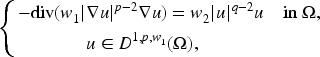
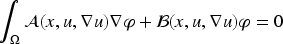
In this article, we study qualitative and quantitative properties of weak solutions to the following equation:
for weights and critical for the weighted Sobolev embedding from (defined before Theorem 4) into . In particular, we are interested in the point-wise asymptotic behavior of a solution to (1).
The main motivation behind studying this problem comes from the results in Castro (2021), where the existence of extremals to a Sobolev inequality with monomial weights was analyzed (see also Cabré & Ros-Oton, 2013; Castro, 2017). It is known that extremals to a weighted Sobolev inequality can be viewed as positive solutions to (1) for appropriate weights , and our goal is to obtain as much information as possible regarding said extremals and, in general, of solutions to (1).
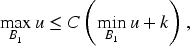
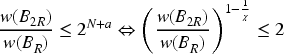
The functions will be weight functions, meaning locally Lebesgue integrable nonnegative functions over satisfying at least the following two conditions: if we abuse the notation and we also write as the measure induced by , that is, , we require that is a doubling measure in , that is, there exists a doubling constant such that
holds for every (open) ball such that , where denotes the ball with the same center as , but with its radius multiplied by . The smallest possible for which (2) holds for every ball will be denoted by from now on. Additionally, we will suppose that
where denotes the -dimensional Lebesgue measure. Observe that these two conditions ensure mutual absolute continuity between the measures and .
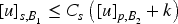
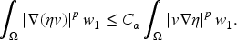
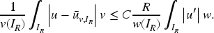
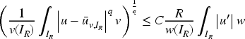
In addition to (2) and (3), we will suppose that the weight satisfies the following local Poincaré inequality: if we write then
Local weighted -Poincaré inequality: There exists such that if then for all balls of radius one has
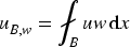
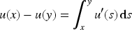
where
is the weighted average of over .
As it can be seen in Heinonen et al. (2006, Chapter 20), when a weight function satisfies (2), (3), and (4), then is -admissible, that is, it also satisfies the following properties:
Uniqueness of the gradient: If satisfy
for some , then .
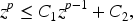
Local Poincaré–Sobolev inequality: There exist constants and such that for all balls one has
for bounded .
Local Sobolev inequality: There exist constants and (same as above) such that for all balls one has
for .
The value of is a dimensional constant associated with the weight , namely, it can be seen that if is a doubling weight then
for , and if we denote then we can take in (5) and (6).
An important class of -admissible weights is the class of Muckenhoupt weights . A weight belongs to for if there exists a constant such that for any ball
where as before denotes the Lebesgue measure in . See Heinonen et al. (2006, Chapter 15) for more details.
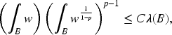
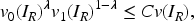
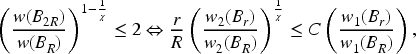
Regarding the weight , in addition to satisfy (2) and (3) (in particular, also satisfies (7) for ), we require that the following compatibility condition with the weight is met: there exists such that
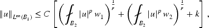
holds for all balls . From Franchi et al. (1994), see also Björn (2001, Theorem 7), we know that if , is -admissible, is doubling, and (8) is satisfied, then the pair of weights satisfy the -local Poincaré–Sobolev inequality
and the -local Sobolev inequality
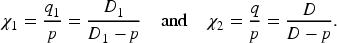
As it will be useful later we write and . Notice that this comes from (8) and in general it has nothing to do with , the dimensional constant associated with the doubling weight mentioned before.
In fact, it can be seen that either (9) or (10) implies (8). The idea is to apply (9) (respectively, (10)) to for suitable , see Chanillo and Wheeden (1985) and Franchi et al. (1994, Remark 4.10) for the details.
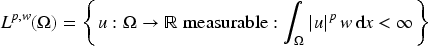
In order to establish the main results of this work, we recall some definitions regarding weighted spaces. For an admissible weight , we consider the weighted Lebesgue space
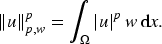
equipped with the norm
In what follows, we will omit writing when there is no confusion about the variable of integration.
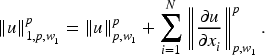
The -admissibility of is useful to have a proper definition for weighted Sobolev spaces: for an open set , we define the weighted Sobolev space
equipped with the norm
As we mentioned before, the goal of this work is to obtain point-wise estimates at infinity for solutions to (1). To do so, we first study the local regularity of weak solutions in the following quasi-linear problem:
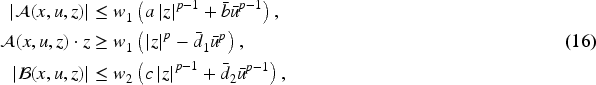
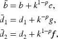
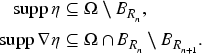
where and are functions verifying the Serrin-like conditions
for a constant and measurable functions satisfying
where and for some essentially bounded, almost everywhere positive function . One of their results shows that every eigenfunction associated with the first eigenvalue is bounded in and has a constant sign.
We are now ready to state the main results of this work. From this point onward, the functions will be nonnegative locally integrable weight functions satisfying (2) and (3), will satisfy the local weighted -Poincaré inequality (4) and the pair will verify the compatibility condition (8). We will also suppose that .
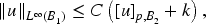
The first result of this work shows that weak solutions to (11) are locally bounded.
Suppose that there exists such that (H) is satisfied, then there exists a constant depending on the norms of such that for any weak solution to (11) in , we have
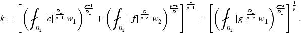
where
and for and , we write
We have chosen to exhibit the local regularity results only for the case as the general case can be easily obtained by a suitable scaling argument.
Next, we consider the case and we show that weak solutions are in for every .
Suppose that (H) is satisfied for , then there exists a constant depending on the norms of such that for any weak solution to (11) in satisfies
Finally, we show that the Harnack inequality holds for nonnegative weak solutions to (11).
Harnack inequality
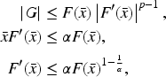
Under the same hypotheses of Theorem 1 with the additional assumption that is a nonnegative weak solution of in , then
where and are as in Theorem 1.
It is worth emphasizing that, while the results in Theorems 1 to 3 may be anticipated in light of the foundational works of Serrin (1964) and Kenig–Fabes–Serapioni (Fabes et al., 1982), to the best of our knowledge, they have not been explicitly established in the literature at this level of generality.
With the aid of the above theorems, we are able to study (1) and to obtain a general result regarding the behavior at infinity of solutions. To do that, we will suppose that in addition to the above conditions, both weights verify global Sobolev inequalities, that is, there exists a constant such that
for and
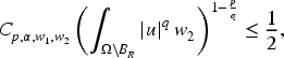
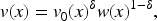
for as in (8), and all . Under these assumptions, and if we define as the closure of under the (semi) norm then embeds continuously into both and and we are able to prove
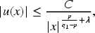
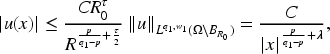
Decay
Suppose is a weak solution to (1). Then, there exists , , and such that
for all in .
It is important to mention that this decay behavior is not optimal, but it can be used as a starting point to obtain better results. This could be done with the aid of a comparison principle and the construction of a suitable barrier function depending on the weights .
The rest of this article is dedicated to the proofs of the above results. In Section 2, we study (11) and obtain the proofs of Theorems 1 to 3, whereas in Section 3, we turn to the proof of Theorem 4. Finally, in Section 4, we show that the above results apply to the class of monomial weights studied in Castro (2017).
Local Estimates
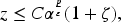
Throughout the different proofs in this section, we will use the dimensional constants of the weights, denoted , as well as the local Sobolev exponents and for given by (8). With these notations, we also have
for some constant depending on and . With the aid of Serrin (1964, Lemma 2), we obtain
which gives
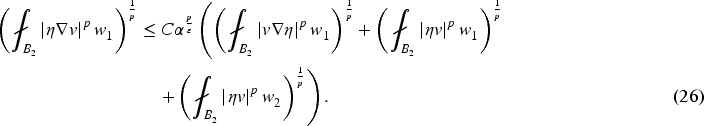
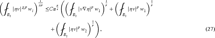
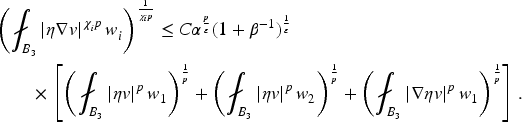
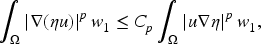
Now, by (6) and (10), the local Sobolev inequalities for the pairs and , respectively, we obtain
where we recall that and .
To continue we consider a sequence of cut-off functions as follows: we take such that in and , where . If one recalls that both weights are doubling so that , we deduce from (27) that (after passing to the limit )
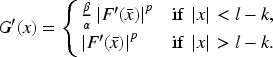
which is valid for all . Recall the definition of given by (13), that is,
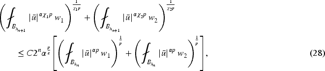
and observe that if then
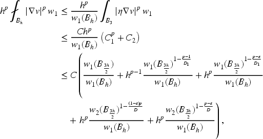
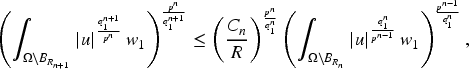
for . Therefore, if we select in (28), we are led to
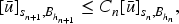
where . Since , then and are convergent series, so we can iterate the above inequality to obtain
for some constant independent of . After passing to the limit , we obtain
and the result follows.
Proof of Theorem 2.
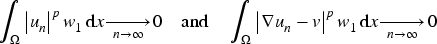
Thanks to the interpolation inequality in , it is enough to find a sequence for which one has
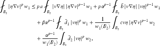
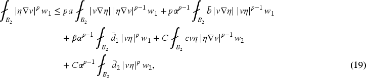
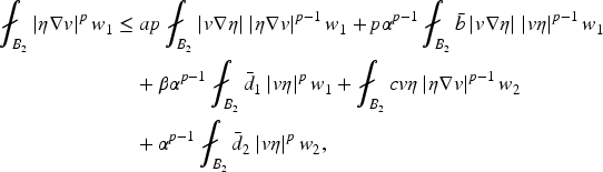
where . As in the proof of Theorem 1, by using the test function , we arrive at the inequality
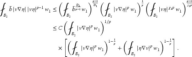
however, since , we cannot apply the same estimates from (20) to (22) directly. Instead, we firstly estimate the term involving as follows:
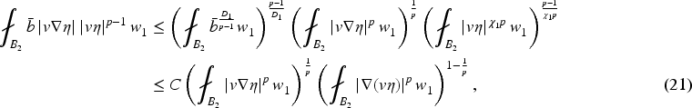
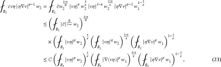
For the terms involving and , we consider , and for each we let and proceed as follows:
Similarly, if for , we have
and
Because , , and then for any , we can find such that
therefore, for any , we can find sufficiently small and a constant such that
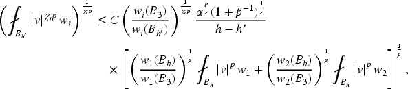
The above inequality allows us to use Serrin (1964, Lemma 2) once again and obtain an inequality analogous to (26), namely
the main difference being that the constant is no longer explicit. Nonetheless, we can continue the argument from the proof of Theorem 1 by choosing appropriate cut-off functions to reach
where , and is defined in (13). Observe that while we do not obtain a uniform estimate for , we can still iterate the above to conclude that
and the result is proved.
Proof of Theorem 3.
By Theorem 1, is bounded on any compact subset of , so for any and any the function is a valid test function provided and , where is defined as in Theorem 1.
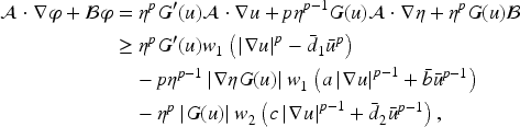
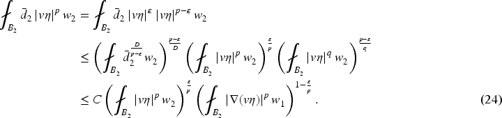
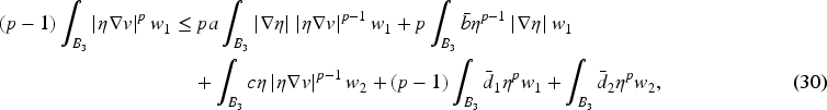
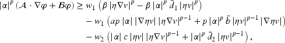
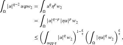
For and we obtain
for any . To continue with the proof denote by and observe that, with the aid of Hölder’s inequality, (30) becomes
where for , we have
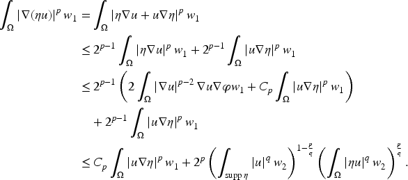
Thanks to Young’s inequality, we deduce that
for some constant . To continue, we estimate and using appropriate . For any such that (not necessarily concentric) we have that and we consider such that in , and .
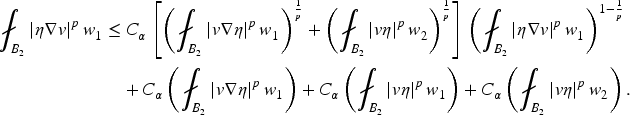
We use such in (31) and (32) and we get the following estimates using Hölder’s inequality and the properties of :
Therefore, one obtains
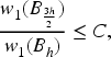
where depends on , , and . We claim that the right-hand side of the above inequality is bounded independently of , indeed because is doubling we have
Hence, for any , each term on the right-hand side is bounded independently of .
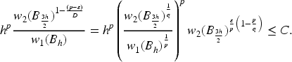
Finally, the local Poincaré–Sobolev inequalities (5) and (9) tell us that
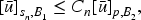
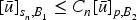
for any ball and both . We conclude that
where is a constant independent of , in other words, . If we denote by as the least possible in (33) then the John–Nirenberg lemma for doubling measures (Heinonen et al., 2006, Appendix II) tells us that there exist constants such that
for all balls . In particular, this gives
and because we have obtained
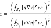
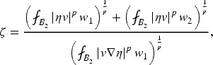
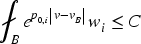
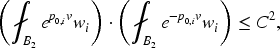
Denote by and observe that
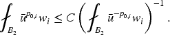
holds for both because and Hölder inequality. Therefore, if we denote by then the inequality above implies
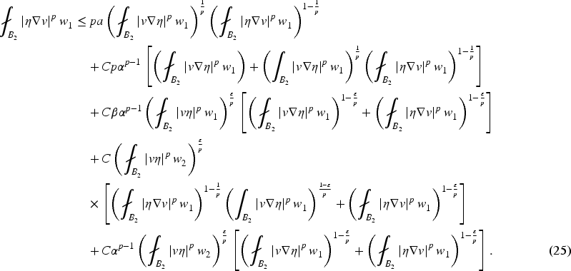
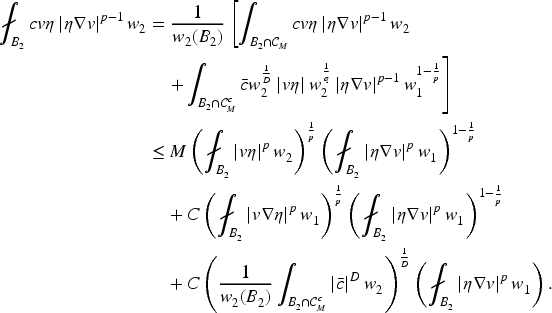
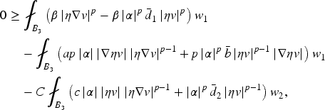
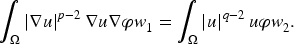
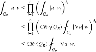
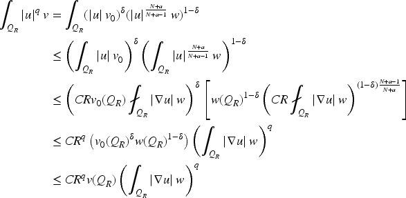
The rest of the proof consists in using for as test function and for given by . This gives
which after integrating over becomes
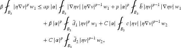
where . Depending on , we have:
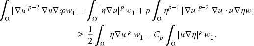
If then
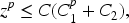
and if we proceed as in the proof of Theorem 1 to estimate each integral on the right-hand side, we obtain
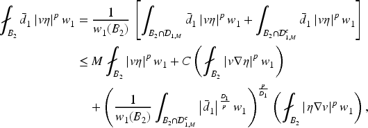
If is such that in for with then
but since , we have
hence, for , we have
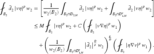
Similarly, for one has
And if then one obtains
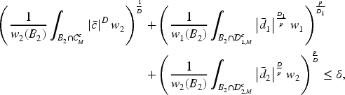
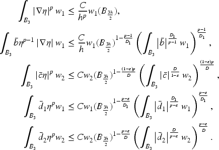
If we observe that and , then we can repeat the iterative argument from the proof of Serrin (1964, Theorem 5) to deduce that (35) and (36) imply
for some chosen appropriately, whereas (37) will give
Finally, we can use (34) to obtain a constant depending on the structural parameters such that
and because we conclude by letting .
Behavior at Infinity
In this section, we obtain a decay estimate for weak solutions to the equation
where the set (bounded or not) is such that there exists a constant for which the global weighted Sobolev inequalities (14) and (15) hold. With the aid of the results regarding the equation , we are able to prove that weak solutions to (38) are locally bounded.
Let be a weak solution of
Then for every such that there exists such that
Observe that equation (38) can be written in the from for , and . Firstly, from Theorem 2, we know that if then for every and the weak solution satisfies
and depends on and on . But because and the weights verify (8) then the local Sobolev inequality (10) holds. Therefore , hence . In particular, this shows that for every and as a consequence for every . Therefore, we can now use Theorem 1 to conclude that
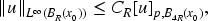
where depends on and the norm of in .
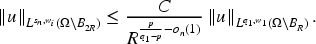
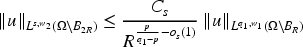
Now we estimate the decay of the norm of weak solutions as one leaves the set .
Suppose is a weak solution of (38), then there exists and such that for one has
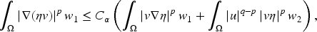
Observe that for any the function is a valid test function in
On the one hand, using Young’s inequality, we can find such that
On the other hand, since , we can write
hence
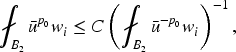
Therefore, the global Sobolev inequality (15) tells us that there exists a constant such that
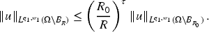
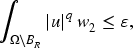
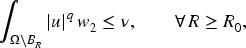
We now choose . First of all, because is finite for any given we can find such that
for any . Hence, we select such that
and we suppose that from now on. We consider , such that , for , for , and . If we use such in (39), we obtain a constant independent of such that
and if we take for , the above inequality gives , which after iterating it gives
Because then one can find such that the above can be written as
Hence
and the result is proved for .
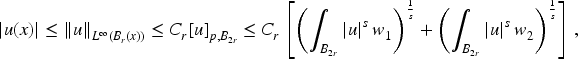
Suppose that is a weak solution of
Then for each there exists (depending on ) and such that
for both and . In the above estimate, is a quantity that goes to as .
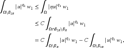
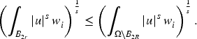
Firstly notice that thanks to the interpolation inequality it is enough to exhibit a sequence such that
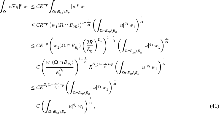
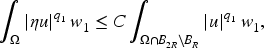
Observe that in the context of (11) we can view (42) as where , and . The assumption tells us that is a valid test function and we can follow the notation of the proof of Theorem 1. Moreover, since we can further suppose that is arbitrary in the definition of both and . Starting with (18) we now integrate over to obtain
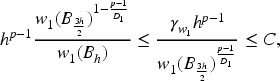
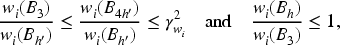
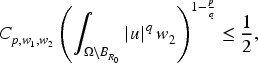
Consider the value of given in Lemma 2, and suppose that . Fix so that and use Lemma 1 to obtain
for any . If we consider , then by geometric considerations we deduce that hence
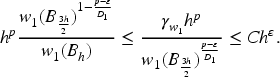
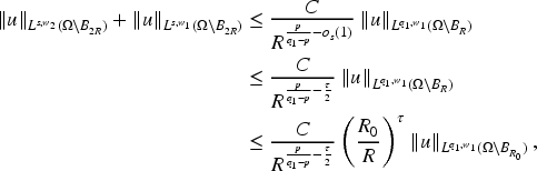
Now we fix large enough so that in Lemma 3, where is taken from Lemma 2, by doing that we obtain
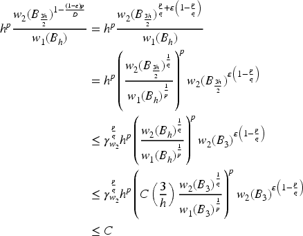
therefore, by putting all the above estimates together, we obtain
for some constant independent of , and the result is proved for .
Monomial Type Weights
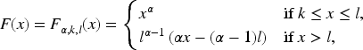
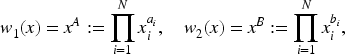
In this section, we show that we can apply the main results of this work to a pair of monomial weights: for we define
for .
Observe that, for , the one-dimensional weight belongs to , in particular, is doubling (with doubling constant ) and -admissible if (see Castro & Cornejo, 2023 for the case ). From this observation, it is not difficult to see that is doubling (with doubling constant , for ) and -admissible, and that is also doubling (with doubling constant for ).
for , for all , and satisfying suitable compatibility conditions (see Castro, 2017 for the details). Therefore in order to use Theorems 1 to 4, we only need to verify that (8) is satisfied by these weights. We will check this by using Remark 4, that is, we will show that the pair of weights satisfies the local Sobolev inequality (10) for suitable .
We begin with some lemmas in dimension 1. In what follows will denote an interval contained in of length .
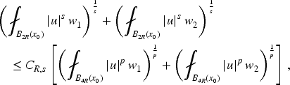
Let , , and . Then for every one has
Write for and let . Starting from
multiply by and integrate over in the variable and then multiply by and integrate over in the variable to obtain
Use Tonelli’s theorem a couple of times on the right-hand side to obtain
so that
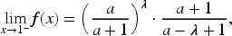
By studying the function for we deduce that if then
and the result follows.
Let and suppose that . Then
for and all .
This follows since the weight is doubling and it satisfies
for , therefore, we can use Lemma 8 to deduce that
from which the local Poincaré–Sobolev inequality follows for and .
Let , , and . Then
and for
for every .
This follows directly from the fact that the local Poincaré–Sobolev inequality implies (8), which in turn implies the local Sobolev inequality (see Remark 4).
The following lemma will allow us to interpolate between the cases and .
Suppose that and that then for , , and there exists a constant depending solely on and such that
for any interval .
Write and if then the inequality is equivalent to proving that
for every . By homogeneity, it suffices to prove that
is bounded in , which follows by continuity of and because and
since and .
We now consider monomial weights in . In what follows, will be a cube with sides parallel to the coordinate axes and edge-length , that is,
with an interval in of length . Also, from now on we will write and suppose that for all .
For with and consider , where is the th element of the canonical basis of , and . There exists a constant such that for any cube we have
Additionally, if for and we define
then there exists a constant such that
The proof is similar to the proof of Lemma 6, we omit the details.
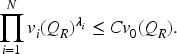
For each consider and then we have
It is enough to consider the case , and in this case observe that if , where each is an interval of length contained in , then by Corollary 1 we have
where and . If we multiply both sides by and integrate over the remaining coordinates we get to
Finally, observe that
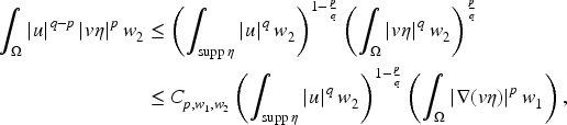
Local Hardy inequality
For with satisfying consider and then we have
If then we can write for , hence by Hölder’s inequality, Proposition 1 and Lemma 7, we obtain
If then
where .
This follows since the weight is doubling and it satisfies
for , therefore we can use Lemma 8 to deduce that
from which the local Sobolev inequality follows.
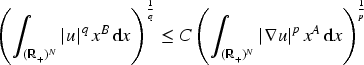
Local Sobolev inequality
For with consider and . If , and then we have
Since we can write for suitable with . Therefore, if we write then
where . Notice that from this choices we can write so that
by Lemma 7 and Propositions 2 and 3
To generalize Proposition 4 to the case , we do the following: from Remark 4 and Proposition 4, we deduce that the weights and satisfy (8) for and , that is,
The weight is doubling with doubling constant , therefore
for . Hence, for , we can write
that is,
thus obtaining the cube version of (8) for . Finally because and by using the doubling property of the weights we can replace the cubes by balls in (50) to get (8) for balls.
Footnotes
Acknowledgments
The author would like to thank the anonymous referees for their suggestions to improve this manuscript.
ORCID iD
Hernán Castro
Funding
The author received no financial support for the research, authorship, and/or publication of this article.
Declaration of Conflicting Interests
The author declared no potential conflicts of interest with respect to the research, authorship, and/or publication of this article.
Notes
A Simpler Version of ( 8 )
References
1.
BjörnJ. (2001). Poincaré inequalities for powers and products of admissible weights. Annales Academiae Scientiarum Fennicae Mathematica, 26(1), 175–188. http://eudml.org/doc/122274
2.
CabréX.Ros-OtonX. (2013). Sobolev and isoperimetric inequalities with monomial weights. Journal of Differential Equations, 255(11), 4312–4336. http://dx.doi.org/10.1016/j.jde.2013.08.010
3.
CastroH. (2017). Hardy–Sobolev-type inequalities with monomial weights. Annali di Matematica Pura ed Applicata, 196(2), 579–598. http://doi.org/10.1007/s10231-016-0587-2
4.
CastroH. (2021). Extremals for Hardy–Sobolev type inequalities with monomial weights. Journal of Mathematical Analysis and Applications, 494(2), 124645. https://doi.org/10.1016/j.jmaa.2020.124645
5.
CastroH.CornejoM. (2023). Poincaré’s inequality and Sobolev spaces with monomial weights. Mathematische Nachrichten, 296(10), 4500–4522. https://doi.org/10.1002/mana.202200100
6.
ChanilloS.WheedenR. L. (1985). Weighted Poincaré and Sobolev inequalities and estimates for weighted Peano maximal functions. American Journal of Mathematics, 107(5), 1191–1226. https://doi.org/10.2307/2374351
7.
FabesE. B.KenigC. E.SerapioniR. P. (1982). The local regularity of solutions of degenerate elliptic equations. Communications in Partial Differential Equations, 7(1), 77–116. https://doi.org/10.1080/03605308208820218
8.
FranchiB.GutiérrezC. E.WheedenR. L. (1994). Weighted Sobolev–Poincaré inequalities for Grushin type operators. Communications in Partial Differential Equations, 19(3–4), 523–604. https://doi.org/10.1080/03605309408821025
HeinonenJ.KilpeläinenT.MartioO. (2006). Nonlinear potential theory of degenerate elliptic equations. Dover Publications, Inc. Unabridged republication of the 1993 original.
11.
PapageorgiouN. S.PudełkoA.RădulescuV. D. (2023). Non-autonomous -equations with unbalanced growth. Mathematische Annalen, 385(3–4), 1707–1745. https://doi.org/10.1007/s00208-022-02381-0
12.
SerrinJ. (1964). Local behavior of solutions of quasi-linear equations. Acta Mathematica, 111, 247–302. https://doi.org/10.1007/BF02391014