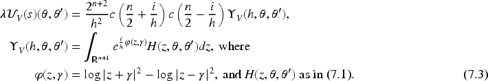
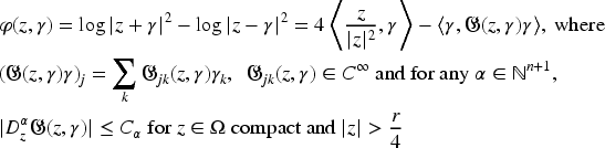
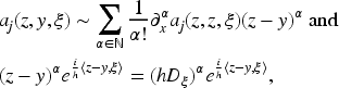
The High Energy Distribution of Scattering Phase Shifts of Schrödinger Operators in Hyperbolic Space

Abstract

We prove a trace formula for the high energy limit of the scattering phase shifts of Schrödinger operators with short range real valued potentials in hyperbolic space; it relates the scattering shifts and the geodesic $X$ -ray transform of the potential. This extends a result of Bulger and Pushnitski for Schrödinger operators in Euclidean space. As an application, we prove that the high energy limit of the phase shifts uniquely determines radial potentials which are monotone and decay super-exponentially. This extends a result of Levinson for potential perturbations of the Euclidean Laplacian to this special class of potentials in hyperbolic space.

Keywords

spectral and inverse spectral problems on manifolds scattering and inverse scattering on manifolds Schrödinger operators scattering phase shifts

1. Introduction

When a wave interacts with a perturbation it undergoes a phase shift and this phenomenon has been well studied by physicists and mathematicians, see for example Bargmann (1949), Berry (1966), Eu (1968), Landau and Lifshitz (1965), Levinson (1949), and Piel and Chrysos (2020), largely for perturbations of the Euclidean Laplacian by real valued radially symmetric potentials, but also for more general perturbations (Birman & Yafaev, 1982; Bulger & Pushnitski, 2012; Gell-Redman & Hassell, 2012; Gell-Redman & Ingremeau, 2019; Gell-Redman et al., 2015; Ingremeau, 2018) of the Euclidean space, and in other settings as well (Christiansen & Uribe, 2021; Kostas & Andersson, 2001). The inverse problem of determining a potential from its phase shifts has also been considered in Bargmann (1949) and Levinson (1949).

The phase shifts are defined to be the logarithm of the eigenvalues of the (relative) scattering matrix, which is a unitary operator. So this is also a spectral problem concerning the distribution of the eigenvalues of a physically meaningful operator which is not self-adjoint. Our main result, Theorem 2.1, establishes a classical-quantum trace formula for Schrödinger operators with short range potentials in hyperbolic space. It relates the high energy distribution of the phase shifts, which are quantum objects, and a measure which is given in terms of the geodesic $X$ -ray transform of the potential, which is a classical quantity. The geodesic $X$ -ray transform of a function (or a tensor) is the map that takes a geodesic to the integral of the function along it. This extends a result of Bulger and Pushnitski (2012), proved for Schrödinger operators in Euclidean space, to hyperbolic space.

Such trace formulas have been proved for the scattering phase shifts of short range real valued potential perturbations of the Euclidean Laplacian, in different régimes. First, Birman and Yafaev (1980, 1982) and Yafaev (2010) for fixed energies, while Bulger and Pushnitski (2012) treated the high energy limit. The case of magnetic Schrödinger operators was considered in Bulger and Pushnitski (2013) in the high energy limit and by Nakamura (2016) for fixed energies, but for more general manifolds. We will not treat magnetic potentials here.

In the case studied here as well as in Bulger and Pushnitski (2012), the potential is an $O (h^{2})$ semiclassical perturbation. In the case where the potential is part of the semiclassical principal symbol of the Hamiltonian, the distribution of scattering phase shifts for the semiclassical Schrödinger operator in Euclidean space was studied by Gell-Redman and Hassell (2012, 2020), Datchev et al. (2014), and by Gell-Redman et al. (2015).

Gell-Redman and Ingremeau (2019) studied the problem for scattering by convex obstacles in Euclidean spaces. Ingremeau (2018) studied compactly supported metric and potential perturbations, and perhaps more importantly, he replaced the assumption of non-trapping with a milder condition on the trapped set. Even in the case of radial potentials, the analysis of the semiclassical problem is very delicate when there is trapping (Berry, 1966). We also mention the work of Christiansen and Uribe (2021) for the semiclassical Schrödinger operator in the case of manifolds with one cylindrical end.

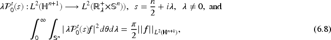
There are several equivalent ways of defining the scattering matrices for the perturbed and unperturbed Laplacians. One can give a dynamical definition in terms of the wave groups and radiation fields as in Lax (2001), Lax and Phillips (1976, 1979, 1980), Nakamura (2016), Sá Barreto (2005), but we will not pursue this here. Instead, we will work in the frequency domain and define the scattering matrix in terms of the asymptotic expansion of generalized eigenfunctions.

It is important to compare the behavior of the eigenvalues of the scattering matrices in the in Euclidean and hyperbolic spaces. In Euclidean space, the unperturbed scattering matrix is the identity, which has only one eigenvalue with infinite multiplicity, independently of the energy. On the other hand, for short range potentials, and for a fixed energy, the scattering matrix of the perturbed Hamiltonian has a countable set of eigenvalues on $S^{1}$ which possibly accumulate at $(1, 0)$ , see for example Birman and Yafaev (1980, 1982) and Yafaev (2010). The scattering matrix of the Laplacian in hyperbolic space $H^{n + 1}$ , defined in equations (2.1) and (2.2) below, has special features. If $g_{0}$ is the metric on $H^{n + 1},$ then for each defining function $x$ of the boundary of $H^{n + 1}$ , $x^{2} g_{0} |_{{x = 0}} = H$ defines a metric on the boundary $\partial H^{n + 1}$ , which is the sphere at infinity. A different choice of a defining function of $\partial H^{n + 1}$ , say $x^{'} = e^{α (x, θ)} x$ , induces a different metric $H^{'} = {x^{'}}^{2} g_{0} |_{x^{'} = 0} = e^{2 α (0, θ)} H$ . This induces a conformal structure on $\partial H^{n + 1}$ and the definition of the scattering matrix has to take into account this conformal structure on $\partial H^{n + 1}$ . For a particular choice of $x$ , the scattering matrix is given by equation (2.4) below and it has a lot of eigenvalues. One can see that for a fixed energy the eigenvalues are dense on $S^{1}$ , and for variable high energies, they actually cover the entire $S^{1}$ . One defines the relative scattering matrix corresponding to a perturbation to be the product of the scattering matrix corresponding to the perturbation times the inverse of the scattering matrix of the unperturbed Laplacian. It turns out that, in the case we are dealing with, the eigenvalues of the relative scattering matrix do not depend on the choice of a conformal representative of the metric on the sphere at infinity. Moreover, its eigenvalues only possibly accumulate at $(1, 0)$ , which is somewhat the opposite of what happens in the Euclidean case.

The proof of our main result, Theorem 2.1, follows the strategy of Bulger and Pushnitski (2012). The main idea is to use the Born approximation to write the relative scattering matrix in two parts, one of which is a semiclassical pseudodifferential operator whose principal symbol is equal to the geodesic $X$ -ray transform of the potential and then use Schatten–von Neumann estimates to show that the contribution of the second term to the trace formula is of lower semiclassical order. In order to do that, we prove Schatten–von Neumann estimates for the Poisson operator in hyperbolic space, which is also known as Helgason Fourier transform (Helgason, 1999; Itoh & Satoh, 2013; Lax, 2001; Zelditch, 1986). These are well known for the Fourier transform in the Euclidean setting and can be found in Chapter 8 of Yafaev (2010) for example, but as far as we can tell, we do not have a reference for them in the case of hyperbolic space.

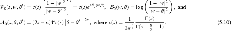
As an application of the trace formula, we show that the high energy limit of the phase shifts uniquely determines a radial potential which is monotone and super-exponentially decaying with respect to the geodesic distance in $H^{n + 1}$ . This result also holds for the Euclidean space using the trace formula proved in Bulger and Pushnitski (2012). Levinson (1949) has shown that, in Euclidean space, the phase shifts for all energies determine a radial potential (with additional assumption about its decay), provided its Schrödinger operator has no negative eigenvalues. Bargmann (1949) has given counter-examples showing that the phase shifts do not determine radial potentials which have negative eigenvalues. Our result does allow negative potentials whose Schrödinger operator may have eigenvalues.

2. The Statement of the Main Results

We define $H^{n + 1}$ , $n \geq 1$ , to be the Riemannian manifold of dimension $n + 1$ which consists of the interior of the ball

B^{n + 1} = {w \in R^{n + 1} : | w | < 1} equipped with the metric g_{0} = \frac{4 d w^{2}}{(1 - | w |^{2})^{2}} .

(2.1)

As in Fefferman and Graham (1985), Mazzeo and Melrose (1987), Melrose (1995) one thinks of

H^{n + 1}

as the interior of a

C^{\infty}

manifold with boundary equipped with a metric which is singular at the boundary

\partial B^{n + 1} = S^{n}

and has a specific asymptotic expansion in a tubular neighborhood of

\partial H^{n + 1}

. The metric

g_{0}

defined in (2.1) is of course singular at

S^{n}

and if we use Euclidean polar coordinates

(r, θ)

r = | w |

and

θ = \frac{w}{| w |}

, it is given by

g_{0} = \frac{4 (d r^{2} + r^{2} d θ^{2})}{(1 - r^{2})^{2}} .

(2.2)

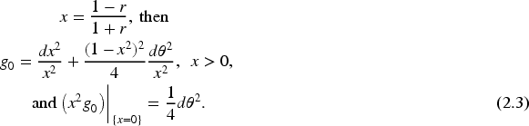
If we set

\begin{matrix} x = \frac{1 - r}{1 + r}, then \\ g_{0} = \frac{d x^{2}}{x^{2}} + \frac{(1 - x^{2})^{2}}{4} \frac{d θ^{2}}{x^{2}}, x > 0, \\ and (x^{2} g_{0}) |_{{x = 0}} = \frac{1}{4} d θ^{2} . \end{matrix}

(2.3)

The function

x

is a defining function of the boundary, in the sense that

x \in C^{\infty}

near

\partial H^{n + 1}

and

x = 0

only at

\partial H^{n + 1}

and

d x \neq 0

\partial H^{n + 1}

. But for example

\tilde{x} = 1 - r

, or

\tilde{x} = e^{ϕ} x

ϕ \in C^{\infty} (H^{n + 1})

, would also be defining functions of

\partial B^{n + 1}

. The induced metric on

S^{n}

, which is given by

(x^{2} g_{0}) |_{x = 0}

depends on the choice of

x

. Vice-versa, as noted in Graham (2000) and Joshi and Sá Barreto (2000), the choice of a conformal representative of

x^{2} g_{0} |_{\partial H^{n + 1}}

determines a unique boundary defining function

ϱ

\partial H^{n + 1}

such that

ϱ^{2} g_{0} = d ϱ^{2} + H (ϱ, θ, d θ)

near

{ϱ = 0}

Let $Δ_{g_{0}}$ denote the Laplacian on $H^{n + 1}$ . It is known that the spectrum of $Δ_{g_{0}}$ is absolutely continuous and equal to $[\frac{n^{2}}{4}, \infty)$ , see for example Isozaki and Kurylev (2014), Lax and Phillips (1976), McKean (1970) and Melrose (1995). If $V$ is real valued and decaying fast enough at infinity, $Δ_{g_{0}} + V$ is self-adjoint and its spectrum consists of an absolutely continuous part $[\frac{n^{2}}{4}, \infty)$ and a finite number of eigenvalues in $(0, \frac{n^{2}}{4})$ , see for example Joshi and Sá Barreto (2000), Mazzeo and Melrose (1987) and Sá Barreto and Wang (2025). We shall work with $Δ_{g_{0}} - \frac{n^{2}}{4}$ which shifts the continuous spectrum to $[0, \infty)$ .

The generalized eigenfunctions of $Δ_{g_{0}} - \frac{n^{2}}{4} + V$ are solutions of

(Δ_{g_{0}} + V - s (n - s)) u (s, w) = 0,

which are bounded but not in

L^{2}

, and have a prescribed asymptotic behavior at infinity, which in this case is the boundary of

H^{n + 1} = S^{n}

, given by powers of the boundary defining function

x

, see equation (5.1) below. Here

s = \frac{n}{2} + i λ,

λ \in R ∖ 0

, and so

s (n - s) = \frac{n^{2}}{4} + λ^{2},

and this choice of spectral parameter is standard in this setting.

This leads to the definition of $A_{V} (s)$ and $A_{0} (s)$ , which are the scattering matrices corresponding to $V$ and $V = 0$ , see (5.3). If we pick $x$ as in (2.3), we have

A_{0} (s) = \frac{Γ (- i λ)}{Γ (i λ)} Δ_{S^{n}}^{i λ}, s = \frac{n}{2} + i λ, λ \in R ∖ 0,

(2.4)

where

Δ_{S^{n}}

is the standard Laplacian on

S^{n}

, see for example Guillopé and Zworski (1995), Joshi and Sá Barreto (2000), and Perry (1989).

The operators $A_{0} (s)$ and $A_{V} (s)$ , which in principle act on $C^{\infty} (S^{n})$ , extend to unitary operators acting on $L^{2} (S^{n})$ with respect to the metric induced by $g_{0}$ at the boundary, and hence their eigenvalues lie on $S^{1}$ , but depend on the choice of $x$ . To overcome this difficulty, we work with the relative scattering matrix $T_{V} (s) = A_{V} (s) A_{0} {(s)}^{- 1}$ . It turns out that $T_{V} (s)$ is unitary and its eigenvalues do not depend on the choice of $x$ . Moreover, $T_{V} (s) = I + E_{V} (s)$ , where $E_{V} (s)$ is a compact operator. Therefore, its eigenvalues lie on the unit circle and only possibly accumulate at $(1, 0)$ .

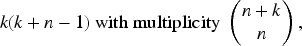
Since the eigenvalues of the Euclidean Laplacian on $S^{n}$ are

k (k + n - 1) with multiplicity (\begin{matrix} n + k \\ n \end{matrix}),

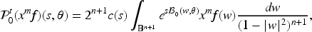
the spectrum of

A_{0} (λ)

given by (2.4) consists of eigenvalues

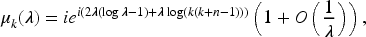
μ_{k} (λ) = \frac{Γ (- i λ)}{Γ (i λ)} {(k (k + n - 1))}^{i λ} with multiplicity (\binom{n + k}{n}) .

(2.5)

For $λ$ fixed, modulo the term involving the gamma function which is independent of $k$ , these are points on $S^{1}$ of the form $e^{i λ \log (k (k + n - 1))}$ and it is well known, see Example 2.4 of Kuipers and Niederreiter (1974), that this is a dense subset of $S^{1}$ , but which is not equidistributed. On the other hand for fixed $k$ , Stirling’s formula (Abramowitz & Stegun, 1972) gives that

\frac{Γ (i λ)}{Γ (- i λ)} = i {(\frac{λ^{2}}{e^{2}})}^{i λ} (1 + O (\frac{1}{λ})) = i e^{2 i λ (\log λ - 1)} (1 + O (\frac{1}{λ})), as λ \to \infty,

and therefore as

λ

varies, it covers the entire

S^{1}

. If one just takes

λ \in N

, then according to Example 2.8 of Kuipers and Niederreiter (1974), the sequence

μ_{k} (λ) = i e^{i (2 λ (\log λ - 1) + λ \log (k (k + n - 1)))} (1 + O (\frac{1}{λ})),

is equidistributed on

S^{1}

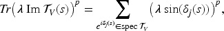
Therefore, while for $λ$ fixed the eigenvalues of $A_{0} (s)$ are dense on $S^{1}$ , the eigenvalues of $T_{V} (s)$ only possibly accumulate at the point $(1, 0) \in S^{1}$ . At the high energy limit, the eigenvalues of $A_{0} (s)$ cover $S^{1}$ and our goal is to describe the effect potential perturbations have on these eigenvalues. We denote the eigenvalues of $T_{V} (s)$ by

\begin{aligned} e^{i δ_{j} (s)}, δ_{j} (s) \in [- π, π), j \in N, & counted with multiplicity, and we know that \\ δ_{j} (s) \to 0 as j \to \infty . \end{aligned}

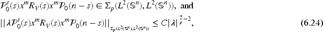
The numbers

δ_{j} (s)

will be called the relative scattering phase shifts. We will show that

| | T_{V} (s) - I | |_{L (L^{2} (H^{n + 1}))} \leq C | λ |^{- 1} for s = \frac{n}{2} + i λ, λ \in R, | λ | > C,

see equation (6.15) below. So it follows that

| e^{i δ_{j} (s)} - 1 | \leq C | λ |^{- 1},

for

λ \in R

and

| λ | > C

. In particular, for

λ \in R ∖ 0

| λ | >> 1

| δ_{j} (\frac{n}{2} + i λ) | \leq | \sin δ_{j} (\frac{n}{2} + i λ) | \leq C | λ |^{- 1}

. We set

λ = \frac{1}{h}

and for

s = \frac{n}{2} + \frac{i}{h}

, we denote

κ_{j} (h) = δ_{j} (\frac{n}{2} + \frac{i}{h})

. As in Bulger and Pushnitski (2012), we define the following measure

⟨ μ_{h}, f ⟩ = (2 π h)^{n} \sum_{e^{i κ_{j} (h)} \in spec T_{V}} f (\frac{κ_{j} (h)}{h}), f \in C_{0}^{0} (R ∖ 0) .

(2.6)

If one takes $f = χ_{([a, b])}$ , $0 \notin [a, b]$ , (as a limit of continuous functions), this is equivalent to the following counting measure:

(2 π h)^{- n} ⟨ μ_{h}, χ_{[a, b]} ⟩ = # {j : \frac{κ_{j} (h)}{h} \in [a, b] \subset R ∖ 0}, counted with multiplicity.

(2.7)

Our purpose is to study the limit of $μ_{h}$ , as $h ↓ 0$ and we prove the following

Theorem 2.1

Let $m \in (1, \infty)$ and $n \in N$ , $n \geq 1$ . Let $V \in x^{m} L^{\infty} (H^{n + 1})$ be real valued, and let $f \in C^{0} (R)$ be such that $\frac{f (t)}{t^{p}} \in C^{0} (R)$ , for some $p \in N$ with $p > \frac{2 (n - \frac{1}{2})}{m - 1}$ . Then

lim_{h \to 0} ⟨ μ_{h}, f ⟩ = \int_{S^{n}} \int_{R^{n}} f (- 2^{n - 1} X (V) (\frac{ξ}{2}, θ)) d ξ d θ .

(2.8)

V

is bounded and compactly supported, we can take

m = \infty

and

p = 1

. Equation (2.8) can be rephrased as

lim_{h \to 0} ⟨ μ_{h}, f ⟩ = \int_{R} f (t) d ν (t), f \in C_{0}^{\infty} (R ∖ 0),

(2.9)

where the measure

ν

is defined to be

ν (α, β) = meas {(θ, ξ), θ \in S^{n}, ξ \in R^{n}, ⟨ ξ, θ ⟩ = 0 such that - 2^{n - 1} X (V) (\frac{ξ}{2}, θ) \in (α, β) \subset R ∖ 0} .

(2.10)

Here “meas” indicates the Lebesgue measure, and

X (V) (\frac{ξ}{2}, θ)

is the geodesic

X

-ray transform of the potential

V

along the geodesic

σ (\frac{ξ}{2}, θ)

defined in (4.2) below.

As already mentioned, in the case of a potential perturbation of $Δ$ in $R^{n}$ , the analogue of this theorem was proved in Bulger and Pushnitski (2012).

2.1. An Inverse Theorem

We apply Theorem 2.1 to prove that the high energy limit of the phase shifts determines a class of radial potentials in $H^{n + 1}$ . The methods of Levinson (1949) will likely also work in $H^{n + 1}$ , but we are not aware this has been investigated. However, we are only dealing with the high energy limit of the phase shifts and we only recover the measure $ν$ , so it is reasonable to expect that we need to restrict the class of potentials.

We say that a potential $V (w)$ , $w \in H^{n + 1}$ , is radial if it only depends on the distance $d_{g_{0}} (0, w)$ from the origin to $w$ with respect to the metric $g_{0}$ . It follows form equation (5.8) below that $ρ (w) = d_{g_{0}} (w, 0) = \log \frac{1 + | w |}{1 - | w |}$ , where $| w |$ denotes the Euclidean norm of $w$ . So $| w | = \tanh (\frac{ρ}{2})$ . So if $V$ is a radial potential if it can be written it as

V (w) = V (ρ (w)) = V (\log \frac{1 + r}{1 - r}), r = | w |

Moreover, if

w = θ + \frac{t θ + ξ}{t^{2} + | ξ |^{2}}

, then

| w |^{2} = 1 + \frac{1 + 2 t}{t^{2} + | ξ |^{2}}

(see the discussion in Section 4 to understand the change of variables), and so it follows from (4.2) that

X (V) (ξ, θ)

is radial and we define

- 2^{n - 1} X (V) (\frac{ξ}{2}, θ) := G_{V} (r), r = | ξ | .

(2.11)

Theorem 2.2

Let $V_{1}, V_{2} \in C^{1} (H^{n + 1}) ⋂ x^{m} L^{\infty} (H^{n + 1})$ , for all $m > 0$ , be real valued radial potentials which are strictly monotone in the sense that $V_{j}^{'} (r) \neq 0$ if $V_{j} (r) \neq 0$ , $j = 1, 2$ . Let $μ_{h} (V_{j})$ , $j = 1, 2$ be the measure defined in (2.6). If

lim_{h \to 0} ⟨ μ_{h} (V_{1}), f ⟩ = lim_{h \to 0} ⟨ μ_{h} (V_{2}), f ⟩, for all f \in C_{0}^{\infty} (R ∖ 0),

(2.12)

then

V_{1} (w) = V_{2} (w)

for all

w \in H^{n + 1}

Theorem 2.2 allows negative potentials, and the associated Schrödinger operators may in principle have discrete spectrum, and so it covers cases not included in the (possible generalization of the) results of Levinson (1949). The proof of Theorem 2.2 also applies to the Euclidean case and it follows from the trace formula proved in Bulger and Pushnitski (2012).

It follows from (2.12) that $ν_{_{V_{1}}} = ν_{_{V_{2}}}$ , where $ν_{_{V_{j}}}$ is the measure defined by (2.10) corresponding to the potential $V_{j}$ . Notice that these are invariant under measure preserving diffeomorphisms of $S^{n} \times R^{n}$ which also preserve orthogonality. In the case of radial potentials, these become measures on $R$ and the best one can hope to conclude is that $G_{V_{1}} (r) = G_{V_{2}} (r + C)$ . We prove that $G_{V_{1}}$ and $G_{V_{2}}$ have the same range and since they are monotone, it follows that $G_{V_{1}} (0) = G_{V_{2}} (0),$ but then it follows that $G_{V_{1}} (0) = G_{V_{2}} (0) = G_{V_{2}} (C)$ and this implies that $C = 0.$

But since $G_{V_{1}} = G_{V_{2}}$ and the potentials decay super-exponentially, we can conclude that $V_{1} = V_{2}$ , because the $X$ -ray transform is injective for functions in $x^{m} L^{\infty} (H^{n + 1})$ for all $m > 0$ , see Theorem 1.2 and Corollary 1.3 of Chapter 3 of Helgason (1999).

3. An Outline of the Proof of Theorem 2.1

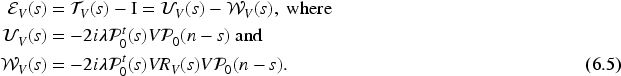
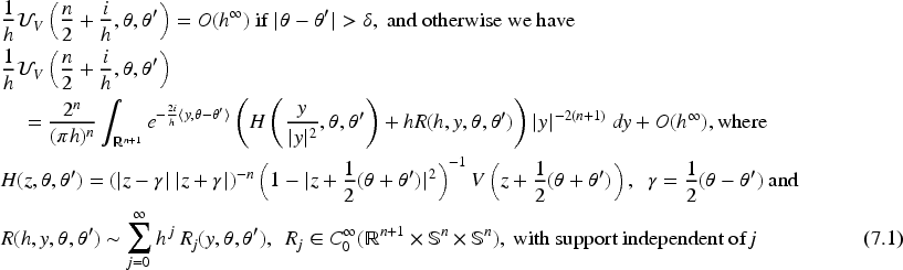
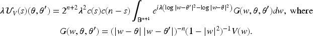
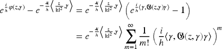
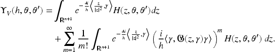
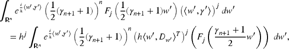
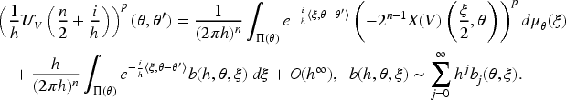
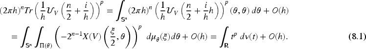
First of all, one needs to recognize that when $f (t) = t^{k}$ , $k \in N$ , Theorem 2.1 is a result about the rescaled trace of the operator ${(T_{V} (\frac{n}{2} + \frac{i}{h}) - I)}^{k}$ . Formally speaking, we first notice that

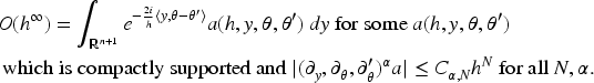
(2 π h)^{n} T r (\frac{1}{h} Im (T_{V} (\frac{n}{2} + \frac{i}{h}) - I))^{k} = (2 π h)^{n} \sum_{e^{i κ_{j} (h)} \in spec T_{V}} (\frac{\sin κ_{j} (h)}{h})^{k}, κ_{j} (h) = δ_{j} (\frac{n}{2} + \frac{i}{h}),

but we use methods of Bulger and Pushnitski (2012) to show that if we replace

\sin κ_{j} (h)

with

κ_{j} (h)

in the formula, the difference between the two is a term of order

O (h)

. We also show that the imaginary part of the operator can be replaced by the operator itself, again with an

O (h)

error. So when

f (t) = t^{k}

, the trace formula says that

(2 π h)^{n} T r (\frac{1}{h} (T_{V} (\frac{n}{2} + \frac{i}{h}) - I))^{k} = \int_{S^{n}} \int_{R^{n}} (- 2^{n - 1} X (V) (\frac{ξ}{2}, θ))^{k} d ξ d θ + O (h) .

For more general functions, the result follows from an application of the Stone–Weierstrass theorem. The idea of proving a trace formula for polynomials first and then using the Stone–Weierstrass theorem to extend it to a more general class of functions is certainly not new and it has been used in several contexts. In the particular case of scattering shifts in appears in several papers, see for example Birman and Yafaev (1980, 1982), Bulger and Pushnitski (2012), Datchev et al. (2014), Gell-Redman et al. (2015), Gell-Redman and Ingremeau (2019), Ingremeau (2018).

The trace of the operator $T_{V} (\frac{n}{2} + \frac{i}{h}) - I$ is equal to the integral of the its Schwartz kernel restricted to the diagonal, and our proof relies on the fact that the Schwartz kernels of the scattering matrices $A_{0} (s)$ and $A_{V} (s)$ can be obtained from the kernels of the respective resolvents (Guillopé & Zworski, 1995; Joshi & Sá Barreto, 2000). In this article, as in Bulger and Pushnitski (2012), we use the Born approximation for $T_{V} (\frac{n}{2} + \frac{i}{h})$ to show that $T_{V} (\frac{n}{2} + \frac{i}{h}) - I = U_{V} (\frac{n}{2} + \frac{i}{h}) - W_{V} (\frac{n}{2} + \frac{i}{h})$ , and that for bounded compactly supported $V$ , $\frac{1}{h} U_{V} (\frac{n}{2} + \frac{i}{h})$ is a semiclassical pseudodifferential operator with principal symbol $- 2^{n - 1} X_{V} (\frac{ξ}{2}, θ)$ . We do not prove that $W_{V} (\frac{n}{2} + \frac{i}{h})$ is a pseudodifferential operator, and instead we use Schatten–von Neumann norm estimates to show that its contribution to the trace is of order $O (h)$ , namely:

(2 π h)^{n} T r (\frac{1}{h} (T_{V} (\frac{n}{2} + \frac{i}{h}) - I))^{k} - (2 π h)^{n} T r (\frac{1}{h} U_{V} (\frac{n}{2} + \frac{i}{h}))^{k} = O (h) .

The Schatten–von Neumann estimates are also needed to extend the result to non-compactly supported short range potentials.

As we will see in Section 5 below, a parametrix for the resolvent gives a parametrix for the scattering matrix, and one should expect to be able to use a more precise parametrix for the semiclassical resolvent such as the ones constructed in Chen and Hassell (2016), Melrose et al. (2014), Sá Barreto and Wang (2016) to directly show that if $V$ is compactly supported, $\frac{1}{h} (T_{V} - I)$ is a semiclassical pseudodifferential operator with principal symbol $- 2^{n - 1} X_{V} (\frac{ξ}{2}, θ)$ . Then Theorem 2.1 would essentially follow from the calculus of semiclassical pseudodifferential operators. This approach would also possibly work in more general situations, including non-trapping asymptotically hyperbolic manifolds, but it would be much more refined and hopefully will be pursued elsewhere.

4. The Geodesic $X$ -Ray Transform in $H^{n + 1}$

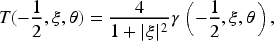
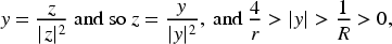
It is well known, see for example Helgason (1999), Lafontaine (2015), that the geodesics of $H^{n + 1}$ are either circles which intersect the boundary $S^{n}$ perpendicularly, or straight lines that go to through the origin. Of course there are many different ways of describing such curves, but in this article they will appear naturally in the computation of the principal symbol of the first Born approximation of the semiclassical scattering matrix by using the inversion map with respect to the sphere $S^{n} :$

\begin{aligned} Q : R^{n + 1} & ∖ 0 ⟶ R^{n + 1} ∖ 0, \\ w ⟼ \frac{w}{| w |^{2}} . \end{aligned}

One can use this map to parametrize all such circles. Let

θ \in S^{n}

and

ξ \in R^{n + 1} ∖ 0

, with

⟨ ξ, θ ⟩ = 0

, and define the curve

t ⟼ Q (t θ + ξ) = \frac{t θ + ξ}{t^{2} + | ξ |^{2}}, where ⟨ ξ, θ ⟩ = 0,

obtained by inverting the line

t \mapsto t θ + ξ

with respect to

S^{n}

. Notice that

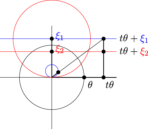
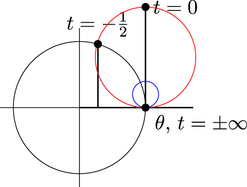
{| \frac{t θ + ξ}{t^{2} + | ξ |^{2}} - \frac{ξ}{2 | ξ |^{2}} |}^{2} = \frac{1}{4 | ξ |^{2}}, provided ξ \neq 0, and ⟨ ξ, θ ⟩ = 0,

and so if we think of

θ = (1, 0, \dots, 0)

and

ξ = (0, ξ_{1}, \dots, ξ_{n + 1})

, this is a parametrization of the circle centered at

(0, \frac{ξ}{2 | ξ |^{2}})

and radius

\frac{1}{2 | ξ |};

the case

ξ = 0

represents a ray in the

θ

direction. The closure of these circles go through the origin at the limits

t \to \pm \infty

and they are tangent to the

θ

-axis and intersect the

ξ

-axis orthogonally. Moreover, since they are contained on the hyperplane defined by

ξ, θ

passing through the origin, we just need to visualize them in two dimensions, see Figure 1.

Figure 1.

Fixed $θ \in S^{1}$ , the Blue (Smaller) and Red (Larger) Circles are the Images of the Lines $t ⟼ t θ + ξ_{j}$ , $ξ_{j} \in R^{2} ∖ 0$ , $⟨ ξ_{j}, θ ⟩ = 0$ , $j = 1, 2$ , Respectively, With Respect to the Map $Q$ . The Circles are Oriented Clockwise and as $\pm t \to \infty$ the Point $Q (t θ + ξ)$ Approaches the Origin From the Right and From the Left, Respectively.

Of course, the map

t ⟼ γ (t, ξ, θ) = θ + \frac{t θ + ξ}{t^{2} + | ξ |^{2}},

(4.1)

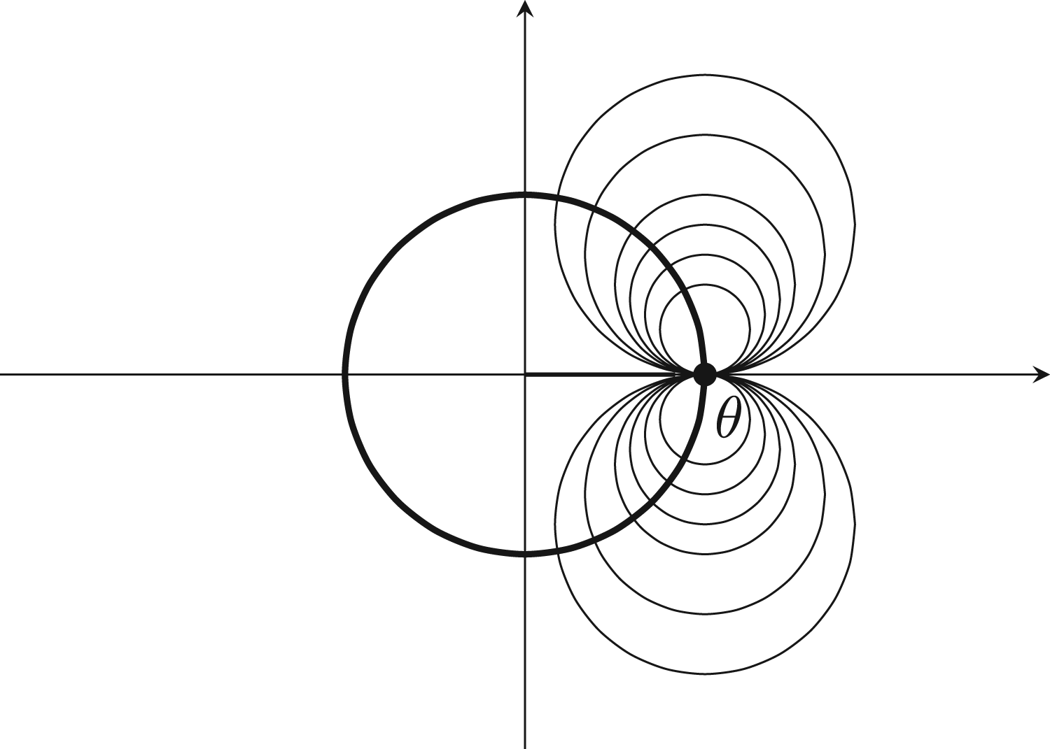
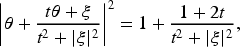
just shifts the circle by

θ

and so it is tangent to the

θ

axis and centered at

(θ, \frac{ξ}{2 | ξ |^{2}})

. Since

⟨ ξ, θ ⟩ = 0

, the circle (4.1) intersects

S^{n}

orthogonally at

θ

, see Figures 2 and 3.

Figure 2.

The Circles of Figure 1 Shifted by $θ$ .

Figure 3.

A Family of Circles $γ (t, ξ, θ)$ , for $θ$ Fixed and for Several Values of $ξ \neq 0$ , With $⟨ ξ, θ ⟩ = 0$ , as $ξ$ Points Upward or Downward.

Notice that

{| θ + \frac{t θ + ξ}{t^{2} + | ξ |^{2}} |}^{2} = 1 + \frac{1 + 2 t}{t^{2} + | ξ |^{2}},

and so these circles intersect

S^{n}

when

t = - \frac{1}{2}

. Moreover, the tangent vector

T (t, ξ, θ) = \partial_{t} γ (t, ξ, θ) = \frac{(| ξ |^{2} - t^{2}) θ - 2 t ξ}{(t^{2} + | ξ |^{2})^{2}},

satisfies

T (- \frac{1}{2}, ξ, θ) = \frac{4}{1 + | ξ |^{2}} γ (- \frac{1}{2}, ξ, θ),

and so

γ (t, ξ, θ)

also intersects

S^{n}

orthogonally when

t = - \frac{1}{2}

. Therefore, for

t \in (- \infty, - \frac{1}{2})

γ (t, ξ, θ)

is a geodesic of

H^{n + 1}

, and all geodesics on

H^{n + 1}

can be parametrized in this way, and we shall denote them by

σ (θ, ξ)

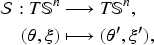
This defines a map of the tangent bundle of $S^{n}$ to itself

\begin{aligned} S : T S^{n} & ⟶ T S^{n}, \\ (θ, ξ) & ⟼ (θ^{'}, ξ^{'}), \end{aligned}

such that

γ (- \frac{1}{2}, ξ, θ) = θ^{'}

and

γ (- \frac{1}{2}, - ξ^{'}, θ^{'}) = θ

. In other words, one follows the geodesic

γ (t, ξ, θ)

, which starts at

θ

in the direction determined by

ξ

until one intersects

S^{n}

again when

t = - \frac{1}{2}

, at

θ^{'}

. The vector

ξ^{'}

is defined to be such the geodesic starting at

θ^{'}

defined by

- ξ^{'}

going backwards intersects

S^{n}

θ

. One can define this map, or perhaps more appropriately, its dual on the cotangent bundle of

S^{n}

, as the scattering relation on

S^{n}

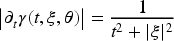
The length of the tangent vector with respect to the Euclidean metric is

| \partial_{t} γ (t, ξ, θ) | = \frac{1}{t^{2} + | ξ |^{2}}

and so if

t \in (- \infty, - \frac{1}{2})

, then

| γ (t, ξ, θ) | < 1

, and the length of the tangent vector with respect to the metric

g_{0}

at the point

θ + \frac{t θ + ξ}{t^{2} + | ξ |^{2}}

is given by

{| \partial_{t} γ (t, ξ, θ) |}_{g_{0}} = 2 {(1 - {| θ + \frac{t θ + ξ}{t^{2} + | ξ |^{2}} |}^{2})}^{- 1} | \partial_{t} γ (t, ξ, θ) | = \frac{- 2}{1 + 2 t}, t \in (- \infty, - \frac{1}{2}) .

Notice that this is positive for

t \in (- \infty, - \frac{1}{2})

, and blows up as

t \to - \frac{1}{2}

, where it intersects the boundary, since the metric

g_{0}

also blows up there.

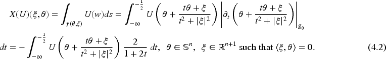
The geodesic $X$ -ray transform of a function $U \in C_{0}^{\infty} (H^{n + 1})$ is defined to be the map which takes a geodesic $γ$ of $H^{n + 1}$ into the integral of $U$ along $γ$ , see for example Chapters 1 and 3 of Helgason (1999). We parametrize such geodesics as in (4.1) and so, we define the geodesic $X$ -ray transform of $U$ along the geodesic $γ (θ, ξ)$ to be

\begin{matrix} X (U) (ξ, θ) = \int_{γ (θ, ξ)} U (w) d s = \int_{- \infty}^{- \frac{1}{2}} U (θ + \frac{t θ + ξ}{t^{2} + | ξ |^{2}}) {| \partial_{t} (θ + \frac{t θ + ξ}{t^{2} + | ξ |^{2}}) |}_{g_{0}} \\ d t = - \int_{- \infty}^{- \frac{1}{2}} U (θ + \frac{t θ + ξ}{t^{2} + | ξ |^{2}}) \frac{2}{1 + 2 t} d t, θ \in S^{n}, ξ \in R^{n + 1} such that ⟨ ξ, θ ⟩ = 0. \end{matrix}

(4.2)

Notice that if

U (w)

is compactly supported in

H^{n + 1}

, so is

X (U) (ξ, θ)

. To see that, suppose that

U (w) = 0

| w |^{2} > 1 - δ

. This implies that

U (θ + \frac{t θ + ξ}{t^{2} + | ξ |^{2}}) = 0

| θ + \frac{t θ + ξ}{t^{2} + | ξ |^{2}} |^{2} - 1 = \frac{2 t + 1}{t^{2} + | ξ |^{2}} > - δ

. But this is equivalent to

{(t + \frac{1}{δ})}^{2} + | ξ |^{2} + \frac{1}{δ} - \frac{1}{δ^{2}} > 0.

It follows that

U (θ + \frac{t θ + ξ}{t^{2} + | ξ |^{2}}) = 0

| ξ | \geq \frac{1}{δ}

and in particular,

X (U) (ξ, θ) = 0

| ξ | \geq \frac{1}{δ}

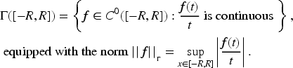
But $X (U)$ is also well defined for any $U$ which is equal to zero outside the ball $B^{n + 1}$ and for which the integral converges. For instance, we will work with the class of functions $U \in x^{m} L^{\infty} (H^{n + 1})$ , $m > 1,$ and we denote

| | U | |_{\infty, m} = sup_{w \in B^{n + 1}} | x {(w)}^{- m} U (w) | .

(4.3)

These norms are equivalent for different choices of the boundary defining function

x

and

| X (U) (ξ, θ) | \leq C | | U | |_{\infty, m} \int_{- \infty}^{- \frac{1}{2}} \frac{| 1 + 2 t |^{m - 1}}{(t^{2} + | ξ |^{2})^{m}} d t \leq C_{m} | | U | |_{\infty, m} (1 + | ξ |)^{- m} .

(4.4)

5. Scattering by a Potential in

H^{n + 1}

We discuss some basic facts about scattering theory on hyperbolic spaces, and we refer the reader to Guillopé and Zworski (1995), Isozaki and Kurylev (2014), Lax (2001), Lax and Phillips (1976, 1979, 1980), Melrose (1995), Mazzeo and Melrose (1987) and Perry (1989) for a more thorough discussion and generalization to asymptotically hyperbolic manifolds. As already mentioned, throughout the article the potential $V$ is assumed to be real valued.

Let $Δ_{g_{0}}$ denote the (positive) Laplacian with respect to the metric $g_{0}$ . Its spectrum is absolutely continuous and equal to $[\frac{n^{2}}{4}, \infty)$ , see for example Isozaki and Kurylev (2014), Lax and Phillips (1976) and McKean (1970). If $V \in x^{m} L^{\infty} (H^{n + 1})$ , $m \in [1, \infty)$ , the spectrum of $Δ_{g_{0}} + V$ , has two parts: a point spectrum consisting of finitely many eigenvalues in $(0, \frac{n^{2}}{4})$ and absolutely continuous part which is also equal to $[\frac{n^{2}}{4}, \infty)$ . There are no embedded eigenvalues, including the bottom of the continuous spectrum, see for example Bouclet (2013), Joshi and Sá Barreto (2000), Mazzeo and Melrose (1987) and Mazzeo (1991).

We consider the generalized eigenfunctions of $Δ_{g_{0}} + V - \frac{n^{2}}{4}$ . Here, as standard, we use $s = \frac{n}{2} + i λ$ , and so $s (n - s) = λ^{2} + \frac{n^{2}}{4}$ . It is known, see for example Joshi and Sá Barreto (2000), Mazzeo and Melrose (1987) and Melrose (1995), that for $V \in x^{m} L^{\infty} (H^{n + 1})$ , $m \in [1, \infty)$ , and any $f \in C^{\infty} (S^{n})$ and $λ \in R ∖ 0$ , there exists a unique $u (s, w) \in C^{\infty} (H^{n + 1})$ such that for $x$ as defined in (2.3),

\begin{aligned} (Δ_{g_{0}} + V - s (n - s))) u (s, w) = 0 in H^{n + 1} and \\ u (s, w) = & x^{s} f (θ) + x^{n - s} g (s, θ) + O (x^{\frac{n}{2} + 1}), w = (x, θ) as x ↘ 0. \end{aligned}

(5.1)

The map

\begin{aligned} P_{V} (s) : & C^{\infty} (S^{n}) ⟶ C^{\infty} (H^{n + 1}) \\ P_{V} (s) f = u (s, w), \end{aligned}

(5.2)

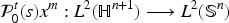
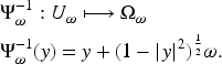
for obvious reasons, is called the Poisson operator, and the map

\begin{aligned} A_{V} (s) : & C^{\infty} (S^{n}) ⟶ C^{\infty} (S^{n}) \\ A_{V} (s) f = g, \end{aligned}

(5.3)

is called the Scattering matrix. We shall use

P_{0} (s)

and

A_{0} (s)

to denote the Poisson operator and the scattering matrix for

V = 0

For $λ \in R ∖ 0$ , $s = \frac{n}{2} + i λ$ , it follows from the definition that

\begin{aligned} P_{V} (s) A_{V} (n - s) = P_{V} (n - s) and \\ A_{V}^{- 1} (s) = A_{V}^{*} (s) = A_{V} (n - s) . \end{aligned}

(5.4)

and so if

s = \frac{n}{2} + i λ

λ \in R ∖ 0

A_{V} (s)

extends to a unitary operator on

L^{2} (S^{n})

with respect to the metric induced on

S^{n}

by the choice of the boundary defining function

x

, as in (2.3).

It was shown in Joshi and Sá Barreto (2000), in greater generality, that for fixed $λ \in R ∖ 0$ , $s = \frac{n}{2} + i λ$ , and the same choice of $x$ , $A_{0} (s)$ and $A_{V} (s)$ are pseudodifferential operators of order zero (truly of complex order $2 i λ$ ), and moreover

A_{V} (s) = A_{0} (s) (I + E_{V} (s)), where E_{V} (s) \in Ψ^{- 1} (S^{n}) .

(5.5)

This notation means that

E_{V} (s)

is a pseudo-differential operator of order

- 1

S^{n}

. This shows that

A_{V} (s)

and

A_{0} (s)

have the same principal part and therefore

T_{V} (s) = A_{V} (s) A_{0} {(s)}^{- 1} = I + E_{V} (s), E_{V} (s) \in Ψ^{- 1} (S^{n}), s = \frac{n}{2} + i λ, λ \in R ∖ 0.

(5.6)

Since $E_{V} (s)$ is a pseudodifferential operator of order $- 1$ , and $S^{n}$ is compact, then by the Sobolev embedding theorem

E_{V} (s) : L^{2} (S^{n}) ⟼ H^{1} (S^{n}) ↪ L^{2} (S^{n})

is a compact operator and therefore the spectrum of

T_{V} (s) = I + E_{V} (s)

consists of eigenvalues contained in

S^{1}

which possibly accumulate at

(1, 0)

. We shall define

T_{V} (s)

to be the relative scattering matrix. This particular relative scattering matrix was also considered by Borthwick and Wang (2024) to study the existence of resonances of

Δ_{g_{0}} + V

Notice that, if we choose two different boundary defining functions $x$ and $\tilde{x}$ such that $x = e^{φ (\tilde{x}, θ)} \tilde{x}$ , then it follows from (5.1) that the corresponding scattering matrices satisfy

A_{∙} (s) f = e^{(s - n) φ (0, θ)} {\tilde{A}}_{∙} (s) (e^{s φ (0, θ)} f), ∙ = V, 0.

Since

A_{0}^{- 1} (s) = A_{0} (n - s)

, it follows that

T_{V} (s) = e^{(s - n) φ (0, θ)} {\tilde{A}}_{V} (s) {\tilde{A}}_{0}^{- 1} (s) e^{(n - s) φ (0, θ)} = e^{(s - n) φ (0, θ)} {\tilde{T}}_{V} (s) e^{(n - s) φ (0, θ)},

and so

T_{V} (s)

and

{\tilde{T}}_{V} (s)

have the same eigenvalues with the same multiplicity, and we conclude that the eigenvalues of

T_{V} (s)

are independent of the choice of

x

5.1. The Kernels of the Poisson Operator and the Scattering Matrix

It is a standard convention to define the resolvent in hyperbolic space as

R_{V} (s) = (Δ_{g_{0}} + V - s (n - s))^{- 1} .

where

s = \frac{n}{2} + i λ

\frac{n^{2}}{4} + λ^{2} = s (n - s)

. When

V

decays fast enough,

R_{V} (s)

is a holomorphic family of bounded operators for

Im λ << 0

, or

Re s >> \frac{n}{2}

. In fact, if

V \in x^{m} L^{\infty} (H^{n + 1})

m \in [1, \infty)

R_{V} (s)

continues meromorphically to

C

, see for example Joshi and Sá Barreto (2000) and Mazzeo and Melrose (1987), with poles of finite multiplicity. These poles are called resonances. In the case where

V \in C_{0}^{\infty} (H^{n + 1})

, Borthwick (2010) and Borthwick and Crompton (2014), proved upper bounds for the counting function of the resonances. Borthwick and Wang (2024) proved the existence of resonances and obtained lower bounds for their counting function.

The Schwartz kernel of the resolvent $R_{∙} (s)$ , $∙ = 0, V$ , is a distribution in $D^{'} (B^{n + 1} \times B^{n + 1})$ , which we denote by $R_{∙} (s, w, w^{'})$ . We know, see for example Lemma 2.1 of Guillopé and Zworski (1995), that in the case $V = 0$ , the Schwartz kernel $R_{0} (s, w, w^{'})$ is given by

\begin{aligned} R_{0} (s, w, w^{'}) & = (\cosh (d_{g_{0}} (w, w^{'})))^{- s} G (s, \cosh (d_{g_{0}} (w, w^{'}))), and for τ > 1, \\ G (s, τ) & = π^{- \frac{n}{2}} 2^{- s - 1} \sum_{j = 0}^{\infty} 2^{- 2 j} \frac{Γ (s + 2 j)}{Γ (s - \frac{n}{2} + j + 1) Γ (j + 1)} τ^{- 2 j}, \end{aligned}

(5.7)

where

d_{g_{0}} (w, w^{'})

is the distance between two points

w, w^{'} \in B^{n + 1}

relative to the metric

g_{0}

. We should remark that the formula in Guillopé and Zworski (1995) is for

H^{n}

instead of

H^{n + 1}

. It is well known Helgason (1999) and Lafontaine (2015) that

d_{g_{0}}

satisfies

\begin{aligned} \cosh (d_{g_{0}} (w, w^{'})) = 1 + \frac{2 | w - w^{'} |^{2}}{(1 - | w |^{2}) (1 - | w^{'} |^{2})} . \end{aligned}

(5.8)

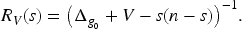
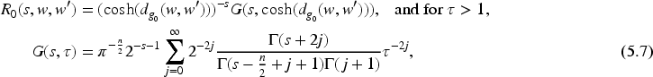
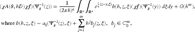
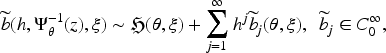
It is proved in Guillopé (1992) and Joshi and Sá Barreto (2000), in much greater generality, that the Schwartz kernels of $P_{∙} (s)$ and $A_{∙} (s)$ , $∙ = 0, V$ , can be obtained from $R_{∙} (s, w, w^{'})$ . We have two copies on the manifold $B^{n + 1}$ , which we denote by $B_{L}^{n + 1} \times B_{R}^{n + 1}$ , where $R$ and $L$ stand for right and left. Let $x_{R}$ and $x_{L}$ denote the function $x$ defined in (2.3) corresponding to each copy. For $s$ fixed, the kernel of $P_{∙} (s)$ is a distribution $P_{∙} (s, w, θ^{'}) \in D^{'} (B^{n + 1} \times S^{n})$ , and similarly the kernel of the scattering matrix $A_{∙} (s, θ, θ^{'}) \in D^{'} (S^{n} \times S^{n})$ , and it turns out that if $w = (x_{L}, θ)$ , and $w^{'} = (x_{R}, θ^{'})$ , then for $∙ = 0, V$ , the kernels of the Poisson operator $P_{∙}$ , its transpose $P_{∙}^{t}$ and the scattering matrix $A_{∙}$ are given by

\begin{aligned} P_{∙} (s, w, θ^{'}) & = R_{∙} (s, w, w^{'}) x_{R}^{- s} |_{{x_{R} = 0}}, \\ P_{∙}^{t} (s, θ, w^{'}) & = x_{L}^{- s} R_{∙} (s, w, w^{'}) |_{{x_{L} = 0}}, and \\ A_{∙} (s, θ, w^{'}) & = (2 s - n) x_{L}^{- s} R_{∙} (s, w, w^{'}) x_{R}^{- s} |_{{x_{L} = x_{R} = 0}} . \end{aligned}

(5.9)

When $V = 0$ , the Schwartz kernel of the Poisson operator and the scattering matrix can be computed directly from (5.7), (5.8) and (5.9). We find that, for $x$ defined in (2.3),

\begin{aligned} P_{0} (s, w, θ^{'}) & = c (s) {[\frac{1 - | w |^{2}}{| w - θ^{'} |^{2}}]}^{s} = c (s) e^{s B_{0} (w, θ)}, B_{0} (w, θ) = \log (\frac{1 - | w |^{2}}{| w - θ |^{2}}), and \\ A_{0} (s, θ, θ^{'}) & = (2 s - n) 4^{s} c (s) {| θ - θ^{'} |}^{- 2 s}, where c (s) = \frac{1}{2 π^{\frac{n}{2}}} \frac{Γ (s)}{Γ (s - \frac{n}{2} + 1)} . \end{aligned}

(5.10)

6. Mapping Properties of the Resolvent and the Poisson Operator

In what follows we shall say that

f \in L^{p} (H^{n + 1}) if | | f | |_{L^{p} (H^{n + 1})}^{p} = \int_{B^{n + 1}} | f (w) |^{p} \frac{2^{n + 1} d w}{(1 - | w |^{2})^{n + 1}} < \infty, 0 < p < \infty .

We will need the following estimate on the operator norm of

R_{0} (s) :

Proposition 6.1 (Proposition 3.2 of Guillarmou, 2005)

If $x$ is a boundary defining function of $H$ , then

| | x^{\frac{1}{2}} R_{0} (\frac{n}{2} + i λ) x^{\frac{1}{2}} | |_{L (L^{2} (H^{n + 1}))} \leq C | λ |^{- 1}, for λ \in R and | λ | > 1.

(6.1)

Here and throughout the article we shall use the notation $| | T | |_{L (H)}$ to indicate the norm of a bounded linear operator $T : H ⟼ H$ , where $H$ is a normed vector space.

Proposition 6.1 implies a similar estimate for $R_{V} (s) :$

Proposition 6.2

If $V \in x L^{\infty} (B^{n + 1})$ , there exist $ϱ > 0$ and $M > 0$ such that

| | x^{\frac{1}{2}} R_{V} (\frac{n}{2} + i λ) x^{\frac{1}{2}} | |_{L (L^{2})} \leq M | λ |^{- 1}, provided λ \in R and | λ | > ϱ .

(6.2)

Proof.

Since $R_{0} (s)$ , $s = \frac{n}{2} + i λ,$ is bounded in $L^{2} (H^{n + 1})$ , for $Im λ < 0$ , the identity

R_{0} (s) (Δ_{g_{0}} + V - s (n - s)) = I + R_{0} (s) V

is valid for

Im λ < 0

, and therefore

x^{\frac{1}{2}} R_{0} (s) x^{\frac{1}{2}} (x^{- \frac{1}{2}} (Δ_{g_{0}} + V - s (n - s)) x^{- \frac{1}{2}}) = I + x^{\frac{1}{2}} R_{0} (s) x^{\frac{1}{2}} V x^{- 1}, Im λ < 0.

We know from (6.1) and from the fact that

x^{- 1} V \in L^{\infty}

, that

| | x^{\frac{1}{2}} R_{0} (s) x^{\frac{1}{2}} V x^{- 1} | |_{L (L^{2} (H^{n + 1}))} \leq C | λ |^{- 1}, λ \in R, | λ | > 1,

and therefore there exists

K > 0

and

ϱ > 0

such that

| | {(I + x^{\frac{1}{2}} R_{0} (s) x^{\frac{1}{2}} V x^{- 1})}^{- 1} | |_{L (L^{2} (H^{n + 1}))} \leq K, provided λ \in R and | λ | > ϱ,

and so we have

x^{\frac{1}{2}} R_{V} (s) x^{\frac{1}{2}} = {(I + x^{\frac{1}{2}} R_{0} (s) x^{\frac{1}{2}} V x^{- 1})}^{- 1} x^{\frac{1}{2}} R_{0} (s) x^{\frac{1}{2}}, for λ \in R and | λ | > ϱ,

and therefore (6.2) follows from (6.1).

6.1. The Born Approximations of

R_{V} (s)

and

T_{V} (s)

As in Birman and Yafaev (1980, 1982) and Bulger and Pushnitski (2012) we will use the first Born approximation for $R_{V} (s)$ and $T_{V} (s)$ to obtain estimates for the operator $E_{V} (s)$ defined in (5.6).

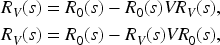
One can easily check the following two identities,

\begin{aligned} R_{V} (s) & = R_{0} (s) - R_{0} (s) V R_{V} (s), \\ R_{V} (s) & = R_{0} (s) - R_{V} (s) V R_{0} (s), \end{aligned}

and combine them to obtain

\begin{aligned} R_{V} (s) - R_{0} (s) = - R_{0} (s) V R_{0} (s) + R_{0} (s) V R_{V} (s) V R_{0} (s), \end{aligned}

(6.3)

which is called the first order Born approximation for

R_{V} (s)

. It follows from (6.3) and (5.9) that

A_{V} (s) - A_{0} (s) = - 2 i λ (P_{0}^{t} (s) V P_{0} (s) - P_{0}^{t} (s) V R_{V} (s) V P_{0} (s)),

and so, after multiplying on the right by

A_{0} {(s)}^{- 1}

and using (5.4) we obtain

T_{V} (s) = A_{V} (s) A_{0} {(s)}^{- 1} = I - 2 i λ P_{0}^{t} (s) V P_{0} (n - s) + 2 i λ P_{0}^{t} (s) V R_{V} (s) V P_{0} (n - s),

(6.4)

which is the first order Born approximation for

T_{V} (s)

. We deduce that

\begin{aligned} E_{V} (s) & = T_{V} (s) - I = U_{V} (s) - W_{V} (s), where \\ U_{V} (s) & = - 2 i λ P_{0}^{t} (s) V P_{0} (n - s) and \\ W_{V} (s) & = - 2 i λ P_{0}^{t} (s) V R_{V} (s) V P_{0} (n - s) . \end{aligned}

(6.5)

We need to obtain suitable norm estimates for the operators

U_{V} (s)

and

W_{V} (s)

An application of Green’s identity, see for example the proof of Proposition 2.1 of Guillopé (1992), shows that

R_{0} (s, w, w^{'}) - R_{0} (n - s, w, w^{'}) = (n - 2 s) \int_{S^{n}} P_{0} (s, w, θ) P_{0}^{t} (n - s, θ, w^{'}) d θ,

(6.6)

On the other hand, Stone’s formula implies that the map

\begin{aligned} P_{0}^{t} (s) : C_{0}^{\infty} (B^{n + 1}) ⟶ C^{\infty} (S^{n} \times R_{+}), \\ (P_{0}^{t} (s) φ) (θ) = & \int_{B^{n + 1}} P_{0}^{t} (s, θ, w) φ (w) \frac{2^{n + 1} d w}{(1 - | w |^{2})^{n + 1}}, s = \frac{n}{2} + i λ, λ > 0, \end{aligned}

(6.7)

induces a surjective isometry

\begin{aligned} λ P_{0}^{t} (s) : & L^{2} (H^{n + 1}) ⟶ L^{2} (R_{λ}^{+} \times S^{n})), s = \frac{n}{2} + i λ, λ \neq 0, and \\ \int_{0}^{\infty} \int_{S^{n}} | λ P_{0}^{t} (s) f |^{2} d θ d λ = \frac{π}{2} | | f | |_{L^{2} (H^{n + 1})}, \end{aligned}

(6.8)

See for example, the proof of Proposition 2.2 of Guillopé (1992). Moreover, it is a spectral representation of

Δ_{g_{0}}

, since

P_{0}^{t} (s) Δ_{g_{0}} φ = s (n - s) P_{0}^{t} (s) φ .

(6.9)

The map $P_{0}^{t} (s)$ is the analogue of the Fourier transform on hyperbolic space, and as already mentioned, it is often called the Helgason Fourier transform. We will follow the strategy of Birman and Yafaev (1980) and Bulger and Pushnitski (2012) and we will need to establish weighted $L^{2}$ and Schatten–von Neumann estimates for the Poisson operator and its transpose. We are not aware of a reference for these estimates in $H^{n + 1}$ , and we prove them here. In the Euclidean space the analogue of these estimates can be found in Chapter 8 of Yafaev (2010). We begin with

Proposition 6.3

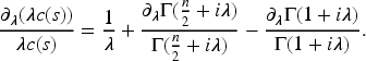
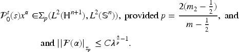
Let $x$ be defined in (2.3) and let $P_{0} (s)$ be the corresponding Poisson operator defined in (5.2), $s = \frac{n}{2} + i λ$ , $λ \in R$ and $| λ | > 1$ , then the following estimates hold:

For any $m \in (0, \infty)$ , there exists $C_{m} > 0$ independent of $s$ such that

| | \partial_{λ} (λ P_{0}^{t} (s)) x^{m} f | |_{L^{2} ((1, \infty)_{λ} \times S^{n})} \leq C_{m} | | f | |_{L^{2} (H^{n + 1})},

(6.10)

and in particular, there exists

C_{m} > 0

independent of

s

such that

\begin{aligned} | | P_{0}^{t} (s) x^{m} f | |_{L^{2} (S^{n})} \leq C_{m} λ^{- 1} | | f | |_{L^{2} (H^{n + 1})}, \\ | | x^{m} P_{0} (s) φ | |_{L^{2} (H^{n + 1})} \leq C_{m} λ^{- 1} | | φ | |_{L^{2} (S^{n})} . \end{aligned}

(6.11)

For $m \in [1, \infty)$ , there exists $C_{m} > 0$ independent of $s$ such that

| | \partial_{θ} (λ P^{t} (s) x^{m}) f | |_{L^{2} ((1, \infty)_{λ} \times S^{n})} \leq C_{m} | | f | |_{L^{2} (H^{n + 1})} .

(6.12)

For $m \in [0, 1]$ the operator $P_{0}^{t} (s) x^{m}$ satisfies

P_{0}^{t} (s) x^{m} : L^{2} (H^{n + 1}) ⟶ H^{m} ((1, \infty)_{λ} \times S^{n}),

(6.13)

For $m \in [\frac{1}{2}, \infty)$ , the operator

P_{0}^{t} (s) x^{m} : L^{2} (H^{n + 1}) ⟶ L^{2} (S^{n})

is compact.

Proof.

We know from (5.10) and from (2.1) that

P_{0}^{t} (x^{m} f) (s, θ) = 2^{n + 1} c (s) \int_{B^{n + 1}} e^{s B_{0} (w, θ)} x^{m} f (w) \frac{d w}{(1 - | w |^{2})^{n + 1}},

c (s)

and

B_{0} (w, θ)

were defined in (5.10). Therefore,

\partial_{λ} (λ P_{0}^{t} (x^{m} f) (s, θ)) = \frac{\partial_{λ} (λ c (s))}{λ c (s)} λ P_{0}^{t} (x^{m} f) (s, θ) + λ P_{0}^{t} (i x^{m} B_{0} (w, θ) f) (s, θ) .

But

\frac{\partial_{λ} (λ c (s))}{λ c (s)} = \frac{1}{λ} + \frac{\partial_{λ} Γ (\frac{n}{2} + i λ)}{Γ (\frac{n}{2} + i λ)} - \frac{\partial_{λ} Γ (1 + i λ)}{Γ (1 + i λ)} .

We recall that the quotient

ψ (z) = \frac{Γ^{'} (z)}{Γ (z)}

is called the digamma function, or the

ψ

function, and it has the following asymptotic expansion

ψ (z) = \log z - \frac{1}{2 z} + o (\frac{1}{z}), as z \to \infty, | \arg z | < π,

see for example Abramowitz and Stegun (1972). Hence,

| \frac{\partial_{λ} (λ c (s))}{λ c (s)} | \leq \frac{C}{λ}, s = \frac{n}{2} + i λ, λ \in R_{+} .

Since

| B_{0} (w, θ) | \leq C | \log (1 - | w |) |, it follows that | x^{m} B_{0} (w, θ) | \leq C for m > 0,

and so it follows from (6.8) that, for

m > 0

\begin{aligned} | | λ P_{0}^{t} (x^{m} f) | |_{L^{2} ((1, \infty)_{λ} \times S^{n})} \leq C | | f | |_{L^{2} (H^{n + 1})} and \\ | | \partial_{λ} (λ P_{0}^{t} (x^{m} f)) | |_{L^{2} ((1, \infty)_{λ} \times S^{n})} \leq C | | f | |_{L^{2} (H^{n + 1})} . \end{aligned}

This proves (6.10) and it implies that

λ P_{0}^{t} (x^{m} f) (λ, θ) \in H^{1} ((1, \infty)_{λ}; L^{2} (S^{n}))

and in particular this implies the first estimate in (6.11). The second estimate follows from the first and this proves the first item.

To prove the second statement, pick coordinates $θ = (θ^{'}, θ_{n})$ , $θ_{n}^{2} = 1 - | θ^{'} |^{2}$ , $| θ_{n} | > ε$ .

\partial_{θ_{j}} P_{0}^{t} (x^{m} f) (s, θ) = s P_{0} (x^{m} \partial_{θ_{j}} B (w, θ) f), j < n,

but

\partial_{θ_{j}} B_{0} (w, θ) = 2 \frac{w_{j} - θ_{j}}{| w - θ |^{2}} + 2 \frac{w_{n} - θ_{n}}{| w - θ |^{2}} \frac{θ_{j}}{θ_{n}},

and since

| θ_{n} | > ε

| \partial_{θ_{j}} B_{0} (w, θ) | \leq \frac{2}{1 - | w |}

, it follows that

| x^{m} \partial_{θ_{j}} B_{0} (w, θ) | \leq C x^{m - 1}

, provided

m > 1

. Since

S^{n}

can be covered by finitely many such charts, (6.12) follows from (6.8), and this proves (6.12).

We have shown that if $m \geq 1$ , $λ P_{0} (s) x^{m} f \in H^{1} ((1, \infty)_{λ} \times S^{n})$ . Now notice that for $x > 0$ and $a > 0$ ,

\begin{aligned} x^{a + i b} = x^{a} (\cos (b \log x) + i \sin (b \log x)), \\ \partial_{a} x^{a + i b} = x^{a + i b} \log x and \partial_{b} x^{a + i b} = i x^{a + i b} \log x, \end{aligned}

and so these are continuous functions up to

x = 0

and so if

Re z > 0

, the function

f (x, z) = {\begin{cases} x^{z} if x > 0, \\ 0 if x = 0 \end{cases}

is holomorphic in

z

(for fixed

x

) and continuous in

x

(for fixed

z

), provided

Re z > 0

We consider the family of operators

F (α) = s P_{0}^{t} (s) x^{α}, Re α > 0.

The family

F (α)

is holomorphic in

α

for

Re α > 0

. Also notice that it follows from (6.8) that

| | s P_{0}^{t} (s) x^{i b} f | |_{L^{2} ((1, \infty)_{λ} \times S^{n})} \leq C | | x^{i b} f | |_{L^{2} (H^{n + 1})} = C | | f | |_{L^{2} (H^{n + 1})} .

(6.14)

This implies that the family

F (α)

is holomorphic for

Re α > 0

and continuous up to

Re α = 0

. We also know from (6.10), (6.12) and (6.14) that

\begin{aligned} | | F (α) f | |_{L^{2} ((1, \infty)_{λ} \times S^{n})} \leq C | | f | |_{L^{2} (H^{n + 1})}, provided Re α = 0, \\ | | F (α) f | |_{H^{1} ((1, \infty)_{λ} \times S^{n})} \leq C | | f | |_{L^{2} (H^{n + 1})}, provided Re α \geq 1. \end{aligned}

It follows from Stein’s interpolation theorem (Stein, 1956), that for

m \in (0, 1)

| | F (α) f | |_{H^{m} ((1, \infty)_{λ} \times S^{n})} \leq C | | f | |_{L^{2} (H^{n + 1})}, provided Re α = m,

and this proves (6.13).

Since $S^{n}$ is compact, if $s = \frac{n}{2} + i λ$ , $| λ | > 1$ , is fixed and $m > \frac{1}{2}$ , it follows from (6.13) and Sobolev restriction theorem that

| | P_{0}^{t} (s) x^{m} f | |_{H^{m - \frac{1}{2}} (S^{n})} \leq C | | f | |_{L^{2} (H^{n + 1})},

and since

m - \frac{1}{2} > 0

, we conclude from the Sobolev embedding theorem that

P_{0}^{t} (s) x^{m}

, as an operator acting on

L^{2} (S^{n})

, is compact for

m > \frac{1}{2}

. To show that the result still holds for

m = Re α = \frac{1}{2}

, notice that

P_{0}^{t} (s) x^{m} f - P_{0}^{t} (s) x^{\frac{1}{2}} f = 2^{n + 1} c (s) \int_{B^{n + 1}} e^{s B_{0} (w, θ)} (x^{m} - x^{\frac{1}{2}}) f (w) \frac{d w}{(1 - | w |^{2})^{n + 1}} .

But we notice that

x^{m} - x^{\frac{1}{2}} = x^{\frac{1}{2}} (x^{m - \frac{1}{2}} - 1) = (m - \frac{1}{2}) x^{\frac{1}{2}} (\log x) q (m, x), q (m, x) := \frac{x^{m - \frac{1}{2}} - 1}{(m - \frac{1}{2}) \log x},

and one can check that

0 < q (m, x) < 1

, for

x \in (0, 1)

and

m > \frac{1}{2}

. It follows that, if

m \in (\frac{1}{2}, 1)

P_{0}^{t} (s) x^{m} f - P_{0}^{t} (s) x^{\frac{1}{2}} f = 2^{n + 1} c (s) \int_{B^{n + 1}} e^{s B_{0} (w, θ)} x^{\frac{1}{2}} (\log x) (m - \frac{1}{2}) q (m, x) f (w) \frac{d w}{(1 - | w |^{2})^{n + 1}},

and it follows from (6.11) that

| | P_{0}^{t} (s) x^{m} f - P_{0}^{t} (s) x^{\frac{1}{2}} f | |_{L^{2} (S^{n})} \leq C (m - \frac{1}{2}) | | f | |_{L^{2} (H^{n + 1})}, m \in (\frac{1}{2}, 1) .

This means that the sequence of compact operators

P_{0}^{t} (s) x^{m}

m > \frac{1}{2}

, converges strongly to

P_{0}^{t} (s) x^{\frac{1}{2}}

m \to \frac{1}{2}

and so

P_{0}^{t} (s) x^{\frac{1}{2}}

is compact , and this ends the proof of the Proposition.

Next we obtain the following estimates for $E_{V} (s) :$

Proposition 6.4

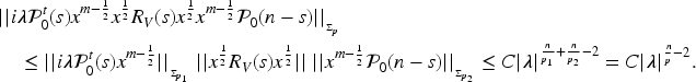
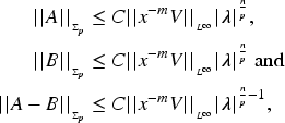
If $m \in (1, \infty)$ and $V \in x^{m} L^{\infty} (H^{n + 1})$ is real valued, then there exist $R > 0$ and $M > 0$ such that

| | T_{V} (\frac{n}{2} + i λ) - I | |_{L (L^{2} (S^{n}))} \leq M | | x^{- m} V | |_{_{L^{\infty}}} | λ |^{- 1}, provided λ \in R, | λ | > R .

(6.15)

Proof.

If $s = \frac{n}{2} + i λ,$ $λ \in R,$ we deduce from (6.11) that there exists $M > 0$ , independent of $λ$ such that if $| λ | > 1,$

| | λ P_{0}^{t} (s) V P_{0} (n - s) | |_{L (L^{2} (S^{n})} = | | λ P_{0}^{t} (s) x^{\frac{m}{2}} (x^{- m} V) x^{\frac{m}{2}} P_{0} (n - s) | |_{L (L^{2} (S^{n})} \leq M | | x^{- m} V | |_{_{L^{\infty}}} | λ |^{- 1},

(6.16)

Similarly, we combine (6.11) and (6.2) to deduce that there exist

R > 0

and

M > 0

, independent of

λ

, such that

| | λ P_{0}^{t} (s) V R_{V} (s) V P_{0} (n - s) | |_{L (L^{2} (S^{n}))} \leq M | | x^{- m} V | |_{_{L^{\infty}}} | λ |^{- 2} for | λ | > R .

(6.17)

6.2. Schatten–von Neumann Estimates for

T_{V} (s)

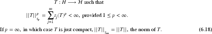
We recall some definitions and results about this topi and we refer the reader to Goh'berg and Krein (1969) and Simon (2005) for more details. If $H$ and $H$ are Hilbert spaces, and $T : H ⟶ H$ is a linear bounded compact operator, then $T^{*} T : H ⟶ H$ is a compact self-adjoint nonnegative operator, and one defines $| T | = \sqrt{T^{*} T}$ . This is also compact, nonnegative and self-adjoint. Let $s_{j} (T)$ denote the eigenvalues of the operator $| T |,$ which are called the singular values of $T$ . They are nonnegative and arranged in such a way that $s_{j} (T) \geq s_{j + 1} (T)$ , and counted with multiplicity, and converge to zero as $j$ goes to infinity.

The Schatten–von Neumann classes $Σ_{p} (H, H)$ , $p \geq 1$ , are defined to be the space of compact operators

\begin{aligned} T : H ⟶ H such that \\ | | T | |_{_{Σ_{p}}}^{p} = \sum_{j = 1}^{\infty} & s_{j} {(T)}^{p} < \infty, provided 1 \leq p < \infty . \\ If p = \infty, in which case & T is just compact, | | T | |_{_{Σ_{\infty}}} = | | T | |, the norm of T . \end{aligned}

(6.18)

This defines a norm, and these spaces are nested

Σ_{p} (H, H) \subset Σ_{q} (H, H) and | | T | |_{_{Σ_{q}}} \leq | | T | |_{_{Σ_{p}}}, provided p \leq q,

and form ideals in the space of bounded operators,

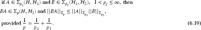
\begin{aligned} A \in & Σ_{p} (H, H_{1}) and B \in L (H_{1}, H_{2}) is a bounded operator with norm | | B | |, \\ then B A \in Σ_{p} (H, H_{2}) and | | B A | |_{_{Σ_{p}}} \leq | | A | |_{_{Σ_{p}}} | | B | | . \end{aligned}

These spaces also satisfy Hölder’s inequality:

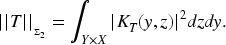
\begin{aligned} if A \in Σ_{p_{1}} (H, H_{1}) and B \in Σ_{p_{2}} (H_{1}, H_{2}), 1 < p_{j} \leq \infty, then \\ B A \in Σ_{p} (H, H_{2}) and | | B A | |_{Σ_{p}} \leq | | A | |_{Σ_{p_{1}}} | | B | |_{Σ_{p_{2}}}, \\ provided \frac{1}{p} = \frac{1}{p_{1}} + \frac{1}{p_{2}} . \end{aligned}

(6.19)

$Σ_{2}$ is also called the class of Hilbert–Schmidt operators and if $T : H ⟶ H$ , and ${φ_{j}, j \in N}$ is an orthonormal basis for $H$ ,

| | T | |_{_{Σ_{2}}} = \sum_{j} | | T φ_{j} | |_{H}^{2}, and is independent of the choice of the basis.

T : L^{2} (X) ⟶ L^{2} (Y)

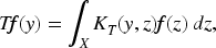
is defined by

T f (y) = \int_{X} K_{T} (y, z) f (z) d z,

then

| | T | |_{_{Σ_{2}}} = \int_{Y \times X} | K_{T} (y, z) |^{2} d z d y .

H = H

, the class

Σ_{1} (H)

consists of trace class operators, and the trace of the operator

T

is given by

T r (T) = \sum_{n = 1}^{\infty} ⟨ T f_{n}, f_{n} ⟩_{H}, where ⟨, ⟩ is the inner product of H and f_{n} is a basis for H,

which converges absolutely and is independently of the choice of the basis.

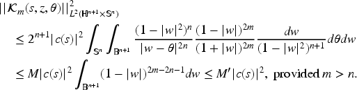
We will need the following Schatten–von Neumann norm estimates for the weighted Poisson operator:

Proposition 6.5

Let $x$ be defined in (2.3) and let $P_{0} (s)$ be defined in (5.2), then the following are true for $s = \frac{n}{2} + i λ$ , provided $λ \in R$ and $| λ | > 1 :$

Let $K_{m} (s, θ, w) \in D^{'} (S^{n} \times B^{n + 1})$ denote the Schwartz kernel of the operator $P_{0}^{t} (s) x^{m}$ . Then, for $m \in (n, \infty)$ , there exists a constant $C_{m}$ independent of $s$ such that

| | K_{m} (s, θ, w) | |_{L^{2} (S^{n} \times H^{n + 1})} \leq C_{m} | λ |^{\frac{n}{2} - 1},

(6.20)

and hence

P_{0}^{t} (s) x^{m} \in Σ_{2} (L^{2} (H^{n + 1}), L^{2} (S^{n}))

and its Hilbert–Schmidt norm satisfies

| | P_{0}^{t} (s) x^{m} | |_{_{Σ_{2} (L^{2} (H^{n + 1}), L^{2} (S^{n}))}} \leq C_{m} | λ |^{\frac{n}{2} - 1} .

(6.21)

If $m \in (\frac{1}{2}, \infty)$ , $p \in [2, \infty)$ , then $P_{0}^{t} (s) x^{m} \in Σ_{p} (L^{2} (H^{n + 1}), L^{2} (S^{n}))$ and

| | P_{0}^{t} (s) x^{m} | |_{_{Σ_{p} (L^{2} (H^{n + 1}), L^{2} (S^{n}))}} \leq C | λ |^{\frac{n}{p} - 1}, provided p > \frac{2 (n - \frac{1}{2})}{m - \frac{1}{2}} .

(6.22)

If $m \in (1, \infty)$ , $p \in [1, \infty)$ and $p > \frac{2 (n - \frac{1}{2})}{m - 1}$ , then $P_{0}^{t} (s) x^{m} P_{0} (n - s) \in Σ_{p} (L^{2} (S^{n}), L^{2} (S^{n}))$ and

| | λ P_{0}^{t} (s) x^{m} P_{0} (n - s) | |_{_{Σ_{p} (L^{2} (S^{n}), L^{2} (S^{n}))}} \leq C | λ |^{\frac{n}{p} - 1},

(6.23)

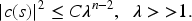
If $m \in (1, \infty)$ and $p \in [1, \infty)$ and $p > \frac{2 (n - \frac{1}{2})}{m - 1}$ , then there exists $ρ > 0$ such that for $| λ | > ρ$ we have

\begin{aligned} P_{0}^{t} (s) x^{m} R_{V} (s) x^{m} P_{0} (n - s) \in Σ_{p} (L^{2} (S^{n}), L^{2} (S^{n})), and \\ | | λ P_{0}^{t} (s) x^{m} R_{V} (s) x^{m} P_{0} (n - s) | |_{_{Σ_{p} (L^{2} (S^{n}), L^{2} (S^{n}))}} \leq C | λ |^{\frac{n}{p} - 2}, \end{aligned}

(6.24)

Proof.

We know from (5.10) that

K_{m} (s, w, θ) = c (s) {(\frac{1 - | w |^{2}}{| w - θ |^{2}})}^{s} x^{m} .

Since

| w - θ |^{2} \geq (1 - | w |)^{2}

s = \frac{n}{2} + i λ

and

x = \frac{1 - | w |}{1 + | w |}

, we have

\begin{aligned} | | K_{m} (s, z, θ) | |_{L^{2} (H^{n + 1} \times S^{n})}^{2} \\ \leq 2^{n + 1} | c (s) |^{2} \int_{S^{n}} \int_{B^{n + 1}} \frac{(1 - | w |^{2})^{n}}{| w - θ |^{2 n}} \frac{(1 - | w |)^{2 m}}{(1 + | w |)^{2 m}} \frac{d w}{(1 - | w |^{2})^{n + 1}} d θ d w \\ \leq M | c (s) |^{2} \int_{B^{n + 1}} (1 - | w |)^{2 m - 2 n - 1} d w \leq M^{'} | c (s) |^{2}, provided m > n . \end{aligned}

We know from Tricomi and Erdélyi (1951) that

\frac{Γ (z + α)}{Γ (z + β)} = z^{α - β} (1 + \frac{(α - β) (α + β - 1)}{2 z} + O (| z |^{- 2})) as | z | \to \infty,

(6.25)

and in particular,

c (\frac{n}{2} + i λ) = \frac{1}{2 π^{n}} λ^{\frac{n}{2} - 1} (1 + O (\frac{1}{| λ |})), as λ \to \infty,

(6.26)

and so for

s = \frac{n}{2} + i λ

| c (s) |^{2} \leq C λ^{n - 2}, λ > > 1.

This proves (6.20), and (6.21) follows from it.

To prove the second item, we proceed as in as in Yafaev (2010). For fixed $s$ , we consider the family

F (α) = P_{0}^{t} (s) x^{α}, α \in C, Re α > 0,

which is holomorphic in

α

. We have shown in Proposition 6.3 and in (6.20) that

$F (α) \in Σ_{\infty} (L^{2} (H^{n + 1}), L^{2} (S^{n}))$ and $| | F (α) | | \leq C λ^{- 1}$ if $Re α \geq \frac{1}{2}$

$F (α) \in Σ_{2} (L^{2} (H^{n + 1}), L^{2} (S^{n}))$ and $| | F (α) | |_{_{Σ_{2}}} \leq C λ^{\frac{n}{2} - 1}$ if $Re α > n$ ,

and so it follows from the three-line theorem for operator valued functions in Schatten classes, see Theorem 2.6 from Chapter 0 of Yafaev (2010) that for all

m_{2} > n

and

m \in (\frac{1}{2}, m_{2})

, and

Re α = m

\begin{aligned} P_{0}^{t} (s) x^{α} \in & Σ_{p} (L^{2} (H^{n + 1}), L^{2} (S^{n})), provided p = \frac{2 (m_{2} - \frac{1}{2})}{m - \frac{1}{2}}, and \\ and | | F (α) |_{_{Σ_{p}}} \leq C λ^{\frac{n}{p} - 1} . \end{aligned}

Since

m_{2} > n

, this proves (6.22).

To prove (6.23) we use that (6.22) holds for $m > 1$ , and for $p_{1}, p_{2} \geq 2$ such that $p_{1}, p_{2} > \frac{2 (n - \frac{1}{2})}{\frac{m}{2} - \frac{1}{2}}$ . Therefore, if $p$ is such that $\frac{1}{p} = \frac{1}{p_{1}} + \frac{1}{p_{2}}$ , then $p \geq 1$ and $\frac{1}{p} < \frac{m - 1}{2 (n - \frac{1}{2})}$ . So we have from (6.19) and (6.22) that

| | i λ P_{0}^{t} (s) x^{m} P_{0} (n - s) | |_{Σ_{p}} \leq | | λ P_{0}^{t} (s) x^{\frac{m}{2}} | |_{_{Σ_{p_{1}}}} | | x^{\frac{m}{2}} P_{0} (n - s) | |_{_{Σ_{p_{2}}}} \leq C | λ |^{\frac{n}{p_{1}}} | λ |^{\frac{n}{p_{2}} - 1} \leq C | λ |^{\frac{n}{p} - 1}

Similarly, to prove (6.24) we write

i λ P_{0}^{t} (s) x^{m} R_{V} (s) x^{m} P_{0} (n - s) = i λ P_{0}^{t} (s) x^{m - \frac{1}{2}} x^{\frac{1}{2}} R_{V} (s) x^{\frac{1}{2}} x^{m - \frac{1}{2}} P_{0} (n - s) .

Again, we use (6.19) and (6.22) and (6.2) to show that, provided

p \geq 1

p > \frac{n - \frac{1}{2}}{m - 1}

, we have

\begin{aligned} | | i λ P_{0}^{t} (s) x^{m - \frac{1}{2}} x^{\frac{1}{2}} R_{V} (s) x^{\frac{1}{2}} x^{m - \frac{1}{2}} P_{0} (n - s) | |_{_{Σ_{p}}} \\ \leq | | i λ P_{0}^{t} (s) x^{m - \frac{1}{2}} | |_{_{Σ_{p_{1}}}} | | x^{\frac{1}{2}} R_{V} (s) x^{\frac{1}{2}} | | | | x^{m - \frac{1}{2}} P_{0} (n - s) | |_{_{Σ_{p_{2}}}} \leq C | λ |^{\frac{n}{p_{1}} + \frac{n}{p_{2}} - 2} = C | λ |^{\frac{n}{p} - 2} . \end{aligned}

Therefore, (6.24) follows from (6.22) and (6.11). This ends the proof of the Proposition.

We apply these results to obtain the following Schatten–von Neumann estimates for $T_{V} (s) - I$ , $U_{V} (s)$ and $W_{V} (s)$ defined in (6.5):

Proposition 6.6

If $V \in x^{m} L^{\infty} (B^{n + 1})$ , $m \in (1, \infty)$ , there exists $ρ > 0$ such that the operators $U_{V} (s)$ and $W_{V} (s)$ , $s = \frac{n}{2} + i λ,$ $λ \in R$ , defined in (6.5) satisfy $U_{V} (s), W_{V} (s) \in Σ_{p} (L^{2} (S^{n}), L^{2} (S^{n}))$ , for any $p \geq 1$ such that $p > \frac{2 (n - \frac{1}{2})}{m - 1}$ and $| λ | > ρ$ . Moreover,

| | U_{V} (s) | |_{_{Σ_{p}}} \leq C | | x^{- m} V | |_{_{L^{\infty}}} | λ |^{\frac{n}{p} - 1} and | | W_{V} (s) | |_{_{Σ_{p}}} \leq C | | x^{- m} V | |_{_{L^{\infty}}} | λ |^{\frac{n}{p} - 2} .

(6.27)

These can also be stated in terms of

T_{V} (s) - I \in Σ_{p} (L^{2} (S^{n}), L^{2} (S^{n}))

and

\begin{aligned} | | T_{V} (s) - I | | |_{_{Σ_{p}}} \leq C | | x^{- m} V | |_{_{L^{\infty}}} | λ |^{\frac{n}{p} - 1} and \\ | | T_{V} (s) - I - U_{V} (s) | | |_{_{Σ_{p}}} \leq C | | x^{- m} V | |_{_{L^{\infty}}} | λ |^{\frac{n}{p} - 2}, \end{aligned}

(6.28)

provided

p \geq 1

p > \frac{2 (n - \frac{1}{2})}{m - 1}

and

| λ | > ρ

Proof.

The proof follows from the simple observation that for $W = x^{- m} V \in L^{\infty} (H^{n + 1})$ , $U_{V} (s)$ satisfies

U_{V} (s) = 2 i λ P_{0} {(s)}^{t} V P_{0} (n - s) = 2 i λ P_{0} {(s)}^{t} x^{\frac{m}{2}} W (z) x^{\frac{m}{2}} P_{0} (n - s), W \in L^{\infty},

and since

m > 1

, one can pick

p_{1} \geq 2

and

p_{2} \geq 2

such that

p_{j} > \frac{2 (n - \frac{1}{2})}{m - \frac{1}{2}}

and

\frac{1}{p} = \frac{1}{p_{1}} + \frac{1}{p_{2}}

and in view of (6.22)

| | U_{V} (s) | |_{Σ_{p}} \leq 2 | | λ P_{0} {(s)}^{t} x^{\frac{m}{2}} | |_{Σ_{p_{1}}} | | W | |_{_{L^{\infty}}} | | x^{\frac{m}{2}} P_{0} (n - s) | |_{Σ_{p_{2}}} \leq C | λ |^{\frac{n}{p} - 1} .

Similarly,

W_{V} (s) = 2 i λ P_{0} {(s)}^{t} V R_{V} (s) V P_{0} (n - s) = 2 i λ P_{0} {(s)}^{t} x^{m - \frac{1}{2}} W (z) x^{\frac{1}{2}} R_{V} (s) x^{\frac{1}{2}} W (z) x^{m - \frac{1}{2}} P_{0} (n - s),

and since

m - \frac{1}{2} > \frac{1}{2}

the same argument applies, fo

| λ | > ρ

such that (6.2) holds.

As a consequence of this we obtain the following, which essentially is Lemma 3.3 of Bulger and Pushnitski (2012):

Proposition 6.7

Let $m \in (1, \infty)$ and $V \in x^{m} L^{\infty} (H^{n + 1})$ , be real valued. There exist $R > 0$ and $C > 0$ such that if $p \in N$ , $p \geq 1$ , and $p > \frac{2 (n - \frac{1}{2})}{m - 1}$ , $s = \frac{n}{2} + i λ$ , $λ \in R$ and $| λ | > R$ , then

| \sum_{e^{i δ_{j} (s)} \in spec T_{V}} (λ δ_{j} (s))^{p} - T r (λ Im T_{V} (s))^{p} | \leq C | | x^{- m} V | |_{L^{\infty}} | λ |^{n - 2} .

(6.29)

Proof.

Since $V$ is real valued, $Im T_{V} (s) = Im (T_{V} - I)$ is compact and self-adjoint,

T r (λ Im T_{V} (s))^{p} = \sum_{e^{i δ_{j} (s)} \in spec T_{V}} (λ \sin (δ_{j} (s)))^{p},

and so (6.29) is equivalent to

S (s) := | \sum_{e^{i δ_{j} (s)} \in spec T_{V}} (λ δ_{j} (s))^{p} - \sum_{e^{i δ_{j} (s)} \in spec T_{V}} (λ \sin (δ_{j} (s)))^{p} | \leq C | | x^{- m} V | |_{L^{\infty}} | λ |^{n - 2} .

In view of (6.15), there exists

R_{0} > 0

such that

| \sin δ_{j} (s) | < C ‖ x^{- m} V ‖_{L^{\infty}} | λ |^{- 1}

, for all

j

, provided

| λ | > R_{0} .

In particular this implies that there exists

C > 0

such that, for

R

large enough,

\frac{1}{2} | δ_{j} (s) | \leq | \sin δ_{j} (s) | \leq | δ_{j} (s) | and | δ_{j} (s) - \sin (δ_{j} (s)) | \leq C | \sin (δ_{j} (s)) |^{3}, | λ | > R .

Therefore

\begin{aligned} | (λ δ_{j} (s))^{p} - (λ \sin (δ_{j} (s))^{p} | = | λ |^{p} | (δ_{j} (s))^{p} - (\sin δ_{j} (s))^{p} | \\ = | λ |^{p} | δ_{j} (s) - \sin (δ_{j} (s)) | Q (| δ_{j} (s) |, | \sin (δ_{j} (s)) |), \end{aligned}

where

Q (x, y)

is a homogeneous polynomial of degree

p - 1

, and therefore,

| λ δ_{j} (s))^{p} - (λ \sin (δ_{j} (s))^{p} | \leq C | λ |^{p} | | \sin (δ_{j} (s))^{p + 2} | .

Again using that

Im T_{V} (s)

is compact and self-adjoint,

\sum_{j} | \sin (δ_{j} (s))^{p + 2} | = | | Im T_{V} | |_{Σ_{p + 2}}^{p + 2} .

So we conclude that, in view of (6.28),

S (h) \leq C | λ |^{p} | | Im T_{V} | |_{Σ_{p + 2}}^{p + 2} \leq C | | x^{- m} V | |_{L^{\infty}} | λ |^{n - 2},

and this ends the proof of the proposition.

We remark that it follows from (5.10), and the fact that $V$ is real valued, that

U_{V}^{*} (s) = - U_{V} (s) and so Im U_{V} (s) = \frac{1}{2 i} (U_{V} (s) - U_{V} {(s)}^{*}) = \frac{1}{i} U_{V} (s),

(6.30)

and as in Lemma 2.2 of Bulger and Pushnitski (2012), we consider the operator

Im T_{V} (s) = \frac{1}{2 i} (T_{V} (s) - T_{V}^{*} (s)) = \frac{1}{i} U_{V} (s) + Im W_{V} (s),

and we have

Proposition 6.8

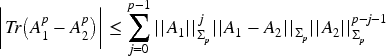
Let $m \in (1, \infty)$ and let $V \in x^{m} L^{\infty} (B^{n + 1})$ be real valued. If $ρ$ is as in Proposition 6.6, then for any $p \in N$ , such that $p \geq 1$ and $p > \frac{2 (n - \frac{1}{2})}{m - 1}$ and $s = \frac{n}{2} + i λ$ , with $λ \in R$ and $| λ | > ρ$ , then

| Tr [{(λ Im T_{V} (s))}^{p} - (λ U_{V} (s))^{p}] | \leq C | | x^{- m} V | |_{_{L^{\infty}}} | λ |^{n - 1} .

(6.31)

Proof.

We present the proof for the convenience of the reader, but we just follow the arguments of Bulger and Pushnitski (2012). First we realize that if $A = λ Im T_{V} (s)$ and $B = \frac{λ}{i} U_{V} (s)$ then

A^{p} - B^{p} = \sum_{j = 0}^{p - 1} A^{j} (A - B) B^{p - 1 - j},

(6.32)

Therefore, by (6.19)

| | A^{p} - B^{p} | |_{_{Σ_{1}}} \leq \sum_{j = 0}^{p - 1} | | A | |_{_{Σ_{p}}}^{j} | | A - B | |_{_{Σ_{p}}} | | B | |_{_{Σ_{p}}}^{p - j - 1} .

(6.33)

But we know from Proposition 6.6 that

\begin{aligned} | | A | |_{_{Σ_{p}}} & \leq C | | x^{- m} V | |_{_{L^{\infty}}} | λ |^{\frac{n}{p}}, \\ | | B | |_{_{Σ_{p}}} & \leq C | | x^{- m} V | |_{_{L^{\infty}}} | λ |^{\frac{n}{p}} and \\ | | A - B | |_{_{Σ_{p}}} & \leq C | | x^{- m} V | |_{_{L^{\infty}}} | λ |^{\frac{n}{p} - 1}, \end{aligned}

and this gives (6.31).

As a consequence of Propositions 6.8 and 6.7 we obtain

Proposition 6.9

Let $m \in (1, \infty)$ and let $V \in x^{m} L^{\infty} (B^{n + 1})$ be real valued. There exists $R > 0$ such that if $p \in N$ , $p \geq 1$ and $p > \frac{2 (n - \frac{1}{2})}{m - 1}$ , and $s = \frac{n}{2} + i λ$ , $λ \in R$ and $| λ | > R$ , then

| \sum_{e^{i δ (s)} \in spec T_{V}} (λ δ_{j} (s))^{p} - T r (λ U_{V} (s))^{p} | \leq C | | x^{- m} V | |_{_{L^{\infty}}} | λ |^{n - 1} .

(6.34)

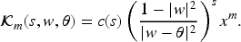
7. The Structure of the Operator

U_{V}

for

V \in C_{0}^{\infty} (B^{n + 1})

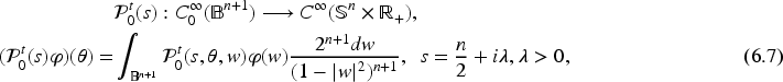
We will show that if $V \in C_{0}^{\infty} (B^{n + 1})$ , then $U_{V} (\frac{n}{2} + \frac{i}{h})$ is in a very special class of semiclassical pseudodifferential operators and in Section 8 we will use the calculus of such operators to prove the trace formulas. We should remark that this result is a particular case of a more general theorem. Notice that the Poisson operator for $H^{n + 1}$ is given by (5.10) and so

(V P_{0} f) (h, w) = c (\frac{n}{2} + \frac{i}{h}) \int_{S^{n}} V (w) e^{(\frac{n}{2} + \frac{i}{h}) B_{0} (w, θ)} f (θ) d θ, B_{0} (w, θ) = \log (\frac{1 - | w |^{2}}{| w - θ |^{2}}) .

V \in C_{0}^{\infty},

then

| w | < 1 - ε

for

ε > 0

, and the phase

B_{0} (w, θ)

is a

C^{\infty}

function and so this is a semiclassical Fourier integral operator, see for example Duistermaat (1974) and Guillemin and Sternberg (2013), associated with the Lagrangian submanifold

Λ

T^{*} (R^{n + 1} \times S^{n})

defined by

Λ = {(w, ς, θ, η) : ς = \partial_{w} B_{0} (w, θ) and η = \partial_{θ} B_{0} (w, θ)} .

U_{V} (\frac{n}{2} + \frac{i}{h})

is the composition of two Fourier integral operators, and the result proved in this section can be thought of as an application of the composition theorem for semiclassical Fourier integral operators, see for example Guillemin and Sternberg (2013), or Hörmander (1994) for regular Fourier integral operators. In this particular case we have an explicit formula and we can prove this result directly using stationary phase methods (which is how the general case is proved), and we start by obtaining an asymptotic expansion in

h

for the Schwartz kernel of

\frac{1}{h} U_{V} (\frac{n}{2} + \frac{i}{h})

Lemma 7.1
If $V \in C_{0}^{\infty} (H^{n + 1})$ and $δ > 0$ , the Schwartz kernel of the operator $\frac{1}{h} U_{V} (\frac{n}{2} + \frac{i}{h})$ defined in (6.5) satisfies
$\begin{aligned} \frac{1}{h} U_{V} (\frac{n}{2} + \frac{i}{h}, θ, θ^{'}) = O (h^{\infty}) if | θ - θ^{'} | > δ, and otherwise we have \\ \frac{1}{h} U_{V} (\frac{n}{2} + \frac{i}{h}, θ, θ^{'}) \\ = \frac{2^{n}}{(π h)^{n}} \int_{R^{n + 1}} e^{- \frac{2 i}{h} ⟨ y, θ - θ^{'} ⟩} (H (\frac{y}{| y |^{2}}, θ, θ^{'}) + h R (h, y, θ, θ^{'})) | y |^{- 2 (n + 1)} d y + O (h^{\infty}), where \\ H (z, θ, θ^{'}) = (| z - γ | | z + γ |)^{- n} {(1 - | z + \frac{1}{2} (θ + θ^{'}) |^{2})}^{- 1} V (z + \frac{1}{2} (θ + θ^{'})), γ = \frac{1}{2} (θ - θ^{'}) and \\ R (h, y, θ, θ^{'}) \sim \sum_{j = 0}^{\infty} h^{j} R_{j} (y, θ, θ^{'}), R_{j} \in C_{0}^{\infty} (R^{n + 1} \times S^{n} \times S^{n}), with support independent of j \end{aligned}$
(7.1)
Here the notation $O (h^{\infty})$ means that it is an integral of the form
$\begin{aligned} O (h^{\infty}) = \int_{R^{n + 1}} e^{- \frac{2 i}{h} ⟨ y, θ - θ^{'} ⟩} a (h, y, θ, θ^{'}) d y for some a (h, y, θ, θ^{'}) \\ which is compactly supported and | (\partial_{y}, \partial_{θ}, \partial_{θ}^{'})^{α} a | \leq C_{α, N} h^{N} for all N, α . \end{aligned}$

Proof.
It follows from (5.10) and (6.5) that the kernel of $U_{V} (s)$ , $s = \frac{n}{2} + i λ$ , $λ \in R ∖ 0,$ satisfies
$\begin{aligned} λ U_{V} (s) (θ, θ^{'}) & = 2^{n + 2} λ^{2} c (s) c (n - s) \int_{B^{n + 1}} e^{i λ (\log | w - θ^{'} |^{2} - \log | w - θ |^{2})} G (w, θ, θ^{'}) d w, where \\ G (w, θ, θ^{'}) = (| w - θ | | w - θ^{'} |)^{- n} (1 - | w |^{2})^{- 1} V (w) . \end{aligned}$
Since $V \in C_{0}^{\infty} (B^{n + 1})$ , and $θ \in S^{n}$ , there exists $ε > 0$ such that $| w - θ | > ε > 0$ , for all $θ \in S^{n}$ , provided $w \in supp (V)$ . We set $w = z + \frac{1}{2} (θ + θ^{'})$ and so
$\begin{aligned} w - θ = z - γ and w - θ^{'} = z + γ, γ = \frac{θ - θ^{'}}{2}, \\ | z - γ | > ε > 0 and | z + γ | > ε > 0. \end{aligned}$
(7.2)

As usual we write $h = λ^{- 1}$ , and so we have
$\begin{aligned} λ U_{V} (s) (θ, θ^{'}) & = \frac{2^{n + 2}}{h^{2}} c (\frac{n}{2} + \frac{i}{h}) c (\frac{n}{2} - \frac{i}{h}) Υ_{V} (h, θ, θ^{'}), \\ Υ_{V} (h, θ, θ^{'}) & = \int_{R^{n + 1}} e^{\frac{i}{h} φ (z, γ)} H (z, θ, θ^{'}) d z, where \\ φ (z, γ) & = \log | z + γ |^{2} - \log | z - γ |^{2}, and H (z, θ, θ^{'}) as in (7.1). \end{aligned}$
(7.3)
In view of (7.2), $φ (z, γ)$ and $H (z, θ, θ^{'})$ are $C^{\infty}$ functions and we can use stationary phase methods to analyze the asymptotic expansion of the integral as $h ↓ 0$ . But
$\frac{1}{4} \nabla_{z} φ (z, γ) = \frac{z + γ}{2 | z + γ |^{2}} - \frac{z - γ}{2 | z - γ |^{2}} = \frac{- 2 ⟨ z, γ ⟩ z + (| z |^{2} + | γ |^{2}) γ}{| z - γ |^{2} | z + γ |^{2}} .$
We find that
$\frac{1}{16} {| \nabla_{z} φ (z, γ) |}^{2} = \frac{| γ |^{2}}{| z - γ |^{2} | z + γ |^{2}} .$
(7.4)
We define the vector field
$\begin{aligned} Z (z, γ) & = \frac{1}{| \nabla_{z} φ |^{2}} ⟨ \nabla_{z} φ, \partial_{z} ⟩ = \frac{1}{| \nabla_{z} φ |^{2}} \sum_{j = 1}^{n + 1} \partial_{z_{j}} φ \partial_{z_{j}} = | γ |^{- 1} R (z, γ), \\ where R (z, γ) & = (- ⟨ z, \frac{γ}{| γ |} ⟩ z + (| z |^{2} + | γ |^{2}) \frac{γ}{| γ |}) \cdot \nabla_{z} \end{aligned}$
and of course $R$ is a vector field with $C^{\infty}$ coefficients in $z$ . Then
$Z e^{\frac{i}{h} φ (z, γ)} = \frac{i}{h} e^{\frac{i}{h} φ (z, γ)} and R e^{\frac{i}{h} φ (z, γ)} = i \frac{| γ |}{h} e^{\frac{i}{h} φ (z, γ)} and$
and so for $N \in N$ ,
$\begin{aligned} {(\frac{i}{h} | γ |)}^{N} Υ_{V} (h, θ, θ^{'}) = \int_{R^{n + 1}} (R (z, γ)^{N} e^{\frac{i}{h} φ (z, γ)}) H (z, θ, θ^{'}) d z \\ = \int_{R^{n + 1}} e^{\frac{i}{h} φ (z, γ)} (R (z, γ)^{T})^{N} H (z, θ, θ^{'}) d z, \end{aligned}$
where $R^{T}$ is the transpose of $R$ . Therefore, if $| γ | > r > 0$ ,
$| {(\frac{i}{h} | γ |)}^{N} Υ_{V} (h, θ, θ^{'}) | \leq C_{N}$
and we conclude that
$if | γ | > δ > 0, then | Υ_{V} (h, θ, θ^{'}) | \leq C (r, N) h^{N} for all N \in N .$
This means that $Υ_{V} (h, θ, θ^{'})$ decays rapidly in $h$ is $| θ - θ^{'} | > δ > 0.$

From now on we assume that $| γ | < r$ , with $r$ small enough. This implies that $\frac{1}{2} | θ + θ^{'} | > 1 - \frac{r}{2}$ and since $V (w) = 0$ for $| w | > 1 - ε$ , we deduce that, on the support of $V$ ,
$| z | = | w - \frac{1}{2} (θ + θ^{'}) | > \frac{1}{2} | θ + θ^{'} | - | w | > ε - \frac{r}{2} > \frac{r}{4} > 0, for r small enough.$
Therefore, we write
$\begin{aligned} φ (z, γ) = \log | z + γ |^{2} - \log | z - γ |^{2} = 4 ⟨ \frac{z}{| z |^{2}}, γ ⟩ - ⟨ γ, G (z, γ) γ ⟩, where \\ (G (z, γ) γ)_{j} = \sum_{k} G_{j k} (z, γ) γ_{k}, G_{j k} (z, γ) \in C^{\infty} and for any α \in N^{n + 1}, \\ | D_{z}^{α} G (z, γ) | \leq C_{α} for z \in Ω compact and | z | > \frac{r}{4} \end{aligned}$
So we write
$\begin{aligned} e^{\frac{i}{h} φ (z, γ)} - e^{- \frac{4 i}{h} ⟨ \frac{z}{| z |^{2}}, γ ⟩} & = e^{- \frac{4 i}{h} ⟨ \frac{z}{| z |^{2}}, γ ⟩} (e^{\frac{i}{h} ⟨ γ, G (z, γ) γ ⟩} - 1) \\ = e^{- \frac{4 i}{h} ⟨ \frac{z}{| z |^{2}}, γ ⟩} \sum_{m = 1}^{\infty} \frac{1}{m!} {(\frac{i}{h} ⟨ γ, G (z, γ) γ ⟩)}^{m} \end{aligned}$
So we conclude that
$\begin{aligned} Υ_{V} (h, θ, θ^{'}) = & \int_{R^{n + 1}} e^{- \frac{4 i}{h} ⟨ \frac{z}{| z |^{2}}, γ ⟩} H (z, θ, θ^{'}) d z \\ + \sum_{m = 1}^{\infty} \frac{1}{m!} \int_{R^{n + 1}} e^{- \frac{4 i}{h} ⟨ \frac{z}{| z |^{2}}, γ ⟩} {(\frac{i}{h} ⟨ γ, G (z, γ) γ ⟩)}^{m} H (z, θ, θ^{'}) d z . \end{aligned}$
Now recall that on the support of the integrand $R > | z | > \frac{r}{4}$ and so we make a change of variables
$y = \frac{z}{| z |^{2}} and so z = \frac{y}{| y |^{2}}, and \frac{4}{r} > | y | > \frac{1}{R} > 0,$
and the integral becomes
$\begin{aligned} Υ_{V} (h, θ, θ^{'}) & = \int_{R^{n + 1}} e^{- \frac{4 i}{h} ⟨ y, γ ⟩} H (\frac{y}{| y |^{2}}, θ, θ^{'}) | y |^{- 2 (n + 1)} d y \\ + \sum_{m = 1}^{\infty} \frac{1}{m!} \int_{R^{n + 1}} e^{- \frac{4 i}{h} ⟨ y, γ ⟩} {(\frac{i}{h} ⟨ γ, G (\frac{y}{| y |^{2}}, γ) γ ⟩)}^{m} H (\frac{y}{| y |^{2}}, θ, θ^{'}) | y |^{- 2 (n + 1)} d y . \end{aligned}$
But notice that
$\frac{i}{h} G_{j k} (\frac{y}{| y |^{2}}, γ) γ_{j} γ_{k} e^{- \frac{4 i}{h} ⟨ y, γ ⟩} = - \frac{i h}{4^{2}} G_{j k} (\frac{y}{| y |^{2}}, γ) \partial_{y_{j}} \partial_{y_{k}} e^{- \frac{4 i}{h} ⟨ y, γ ⟩} .$
and therefore
$\begin{matrix} {(\frac{i}{h} G_{j k} (\frac{y}{| y |^{2}}, γ) γ_{j} γ_{k})}^{m} e^{- \frac{4 i}{h} ⟨ y, γ ⟩} = {(- i \frac{h}{4^{2}})}^{m} P_{m} (y, γ, D) e^{- \frac{4 i}{h} ⟨ y, γ ⟩}, where \\ P_{m} (y, γ, D) = \sum G_{j_{1} k_{1}} G_{j_{2} k_{2}} \dots G_{j_{m} k_{m}} \partial_{y_{j_{1}}} \partial_{y_{k_{1}}} \partial_{y_{j_{2}}} \partial_{y_{k_{2}}} \dots \partial_{y_{j_{m}}} \partial_{y_{k_{m}}} . \end{matrix}$
and then integration by parts gives
$\begin{aligned} \int_{R^{n + 1}} e^{- \frac{4 i}{h} ⟨ y, γ ⟩} {(\frac{i}{h} ⟨ γ, G (\frac{y}{| y |^{2}}, γ) γ ⟩)}^{m} H (\frac{y}{| y |^{2}}, θ, θ^{'}) | y |^{- 2 (n + 1)} d y \\ = {(- \frac{i h}{4^{2}})}^{m} \int_{R^{n + 1}} H (\frac{y}{| y |^{2}}, γ) P_{m} (y, γ, D) e^{- \frac{4 i}{h} ⟨ y, γ ⟩} | y |^{- 2 (n + 1)} d y \\ = {(- \frac{i h}{4^{2}})}^{m} \int_{R^{n + 1}} e^{- \frac{4 i}{h} ⟨ y, γ ⟩} P_{m} (y, γ, D)^{T} (H (\frac{y}{| y |^{2}}, γ) | y |^{- 2 (n + 1)}) d y, \end{aligned}$
where $P_{m} (y, γ, D)^{T}$ denotes the transpose of $P_{m} (y, γ, D)$ . On the other hand, it is shown in Tricomi and Erdélyi (1951) that
$c (\frac{n}{2} + \frac{i}{h}) c (\frac{n}{2} - \frac{i}{h}) \sim \frac{1}{4 π^{n}} h^{2 - n} + \sum_{j = 1}^{\infty} d_{j} h^{2 - n + j}$
and so we have proved the Lemma.

Next we further simplify the formula (7.1) and establish the connection with the geodesic $X$ -ray transform of $V$ .
Proposition 7.2
If $δ > 0$ , the Schwartz kernel of $U_{V}$ satisfies
$\begin{aligned} \frac{1}{h} U_{V} (\frac{n}{2} + \frac{i}{h}, θ, θ^{'}) = O (h^{\infty}), provided | θ - θ^{'} | > δ, and otherwise \\ \frac{1}{h} U_{V} (\frac{n}{2} + \frac{i}{h}, θ, θ^{'}) = \frac{1}{(2 π h)^{n}} \int_{Π (θ)} e^{- \frac{i}{h} ⟨ ξ, θ - θ^{'} ⟩} (H (θ, ξ) + h R (h, θ, ξ)) d μ_{θ} (ξ) + O (h^{\infty}), \\ where Π (θ) = {ξ \in R^{n + 1} : ⟨ ξ, θ ⟩ = 0} and μ_{θ} is the Lebesgue measure on the plane Π (θ), \\ H (θ, ξ) = 2^{n} \int_{R} H (\frac{t θ + \frac{ξ}{2}}{t^{2} + \frac{| ξ |^{2}}{4}}, θ, θ) {(t^{2} + \frac{| ξ |^{2}}{4})}^{- n - 1} d t = - 2^{n - 1} X (V) (\frac{ξ}{2}, θ) as defined in (4.2) \\ and R (h, θ, ξ) \sim \sum_{j = 0}^{\infty} h^{j} R_{j} (θ, ξ), R_{j} (θ, ξ) \in C_{0}^{\infty} (S^{n} \times R^{n + 1}), with support independent of j \\ and O (h^{\infty}) = \int_{Π (ρ)} e^{- \frac{i}{h} ⟨ ξ, θ - θ^{'} ⟩} a (h, θ, ξ) d μ_{θ^{'}} (ξ), for some a (h, θ, ξ) \\ which is compactly supported and | (\partial_{θ}, \partial_{ξ})^{α} a (h, θ, ξ) | \leq C_{N, α} h^{N} for all N, α . \end{aligned}$
(7.5)
Proof.
As observed in Lemma 7.1, if $δ > 0$ and $χ (s) \in C_{0}^{\infty} (R)$ , $χ (s) = 1$ if $| s | < δ$ and $χ (s) = 0$ if $| s | > 2 δ$ , then
$\begin{aligned} \frac{1}{h} U_{V} (\frac{n}{2} + \frac{i}{h}, θ, θ^{'}) \\ = \frac{2^{n}}{(π h)^{n}} \int_{R^{n + 1}} e^{- \frac{2 i}{h} ⟨ y, θ - θ^{'} ⟩} χ (| θ - θ^{'} |^{2}) (H (\frac{y}{| y |^{2}}, θ, θ^{'}) + h R (h, y, θ, θ^{'})) | y |^{- 2 (n + 1)} d y + O (h^{\infty}), \end{aligned}$
with $R (h, y, θ, θ^{'})$ satisfying an expansion as in (7.1). We proceed as in Birman and Yafaev (1980) and Bulger and Pushnitski (2012) and define
$J (θ, θ^{'}) = \frac{θ + θ^{'}}{| θ + θ^{'} |},$
and we observe that since $θ, θ^{'} \in S^{n}$ , $⟨ J (θ, θ^{'}), θ - θ^{'} ⟩ = 0$ and so we can write
$y = t J (θ, θ^{'}) + \frac{ξ}{2}, with ξ such that ⟨ ξ, J (θ, θ^{'}) ⟩ = 0,$
and since $| J (θ, θ^{'}) | = 1$ , we have
$\frac{1}{h} U_{V} (\frac{n}{2} + \frac{i}{h}, θ, θ^{'}) = \frac{1}{(π h)^{n}} \int_{Π (J)} e^{- \frac{i}{h} ⟨ ξ, θ - θ^{'} ⟩} (H (θ, θ^{'}, ξ) + h R (h, θ, θ^{'}, ξ)) d μ_{J} (ξ) + O (h^{\infty}),$
with $Π (J)$ and $μ_{J}$ as defined in (7.5) with $J$ in place of $θ$ ,
$\begin{aligned} H (θ, θ^{'}, ξ) & = \int_{R} χ (| θ - θ^{'} |^{2}) H (\frac{t J (θ, θ^{'}) + \frac{ξ}{2}}{t^{2} + \frac{| ξ |^{2}}{4}}, θ, θ^{'}) {(t^{2} + \frac{| ξ |^{2}}{4})}^{- n - 1} d t, and \\ R (θ, θ^{'}, ξ) & = \int_{R} χ (| θ - θ^{'} |^{2}) R (h, t J (θ, θ^{'}) + \frac{ξ}{2}, θ, θ^{'}) d t, \end{aligned}$
As in the proof of Lemma 7.1, we write the Taylor series expansion of $H (θ, θ^{'}, ξ)$ and $R_{j} (θ, θ^{'}, ξ)$ along the diagonal ${θ = θ^{'}}$
$\begin{aligned} H (θ, θ^{'}, ξ) \sim H (θ, θ, ξ) & + \sum_{| α | = 1} (θ - θ^{'})^{α} T_{α} (h, θ, ξ), with T_{α} \in C^{\infty}, \\ R_{j} (θ, θ^{'}, ξ) \sim R_{j} (θ, θ, ξ) & + \sum_{| α | = 1}^{\infty} (θ - θ)^{α} T_{α, j} (h, θ, ξ), with T_{α, j} \in C^{\infty}, \end{aligned}$
use that
$(θ - θ^{'}) e^{- \frac{i}{h} ⟨ θ - θ^{'}, ξ ⟩} = - \frac{h}{i} \nabla_{ξ} e^{- \frac{i}{h} ⟨ θ - θ^{'}, ξ ⟩},$
and that $χ (| θ - θ^{'} |^{2}) = 1$ near ${θ = θ^{'}}$ and integrate by parts in $ξ$ and use that $J (θ, θ) = θ$ to conclude that
$\begin{aligned} \frac{1}{h} U_{V} (\frac{n}{2} + \frac{i}{h}, θ, θ^{'}) = \frac{1}{(π h)^{n}} \int_{Π (J)} e^{- \frac{i}{h} ⟨ ξ, θ - θ^{'} ⟩} (H (θ, ξ) + h R (h, θ, ξ)) d μ_{J} (ξ) + O (h^{\infty}), \\ H (θ, ξ) = H (θ, θ, ξ), R (h, θ) \sim \sum_{j = 0}^{\infty} h^{j} R_{j} (θ, ξ), R_{j} \in C_{0}^{\infty}, with support independent of j \end{aligned}$
This is not quite the formula we want because the integral is over the hyperplane $Π (J)$ and we want it over $Π (θ)$ and this is clarified by the following Lemma 7.3
Let $θ, γ \in S^{n}$ be such that $| θ - γ | < ε$ is small enough. Let $σ = \frac{θ + γ}{| θ + γ |}$ , $Π (∙)$ and $μ_{∙}$ be defined as in 7.5, $∙ = θ, σ$ . If $F (z) \in C_{0}^{\infty} (R^{n + 1})$ , then
$\begin{aligned} \int_{Π (σ)} e^{\frac{i}{h} ⟨ z, γ - θ ⟩} F (z) d μ_{σ} (z) - \int_{Π (θ)} e^{\frac{i}{h} ⟨ z, γ - θ ⟩} F (z) d μ_{θ} (z) \\ = h \int_{Π (θ)} e^{\frac{i}{h} ⟨ z, γ - θ ⟩} F (h, z, θ) d μ_{θ} (z) + O (h^{\infty}), where \\ F (h, z, θ) \sim \sum_{j = 0}^{\infty} h^{j} F_{j} (z, θ), F_{j} \in C_{0}^{\infty}, with support independent of j \end{aligned}$

Proof.
If $A$ is a linear orthogonal transformation and $γ = A γ^{}$ and $θ = A θ^{}$ , we have
$\begin{aligned} \int_{Π (σ)} e^{\frac{i}{h} ⟨ z, γ - θ ⟩} F (z) d μ_{σ} (z) - \int_{Π (θ)} e^{\frac{i}{h} ⟨ z, γ - θ ⟩} F (z) d μ_{θ} (z) \\ = \int_{Π (σ^{})} e^{\frac{i}{h} ⟨ z, γ^{} - θ^{} ⟩} F (A z) d μ_{σ^{}} (z) - \int_{Π (θ^{})} e^{\frac{i}{h} ⟨ z, γ^{} - θ^{} ⟩} F (A z) d μ_{θ^{}} (z), \end{aligned}$
and so we may assume that $θ = (0, 1)$ and $γ = (γ^{'}, γ_{n + 1})$ , with $| γ^{'} | < ε$ and $| 1 - γ_{n + 1} | < ε$ , for $ε$ small enough. If we denote $z = (z^{'}, z_{n + 1})$ , $z^{'} = (z_{1}, \dots z_{n})$ , and since in this case $σ = \frac{1}{| (γ^{'}, 1 + γ_{n + 1}) |} (γ^{'}, 1 + γ_{n + 1}),$ we have
$Π (θ) = {z \in R^{n + 1} : z_{n + 1} = 0} and Π (σ) = {z \in R^{n + 1} : z_{n + 1} = - \frac{1}{1 + γ_{n + 1}} ⟨ z^{'}, γ^{'} ⟩,$
and so
$\begin{aligned} \int_{Π (θ)} e^{\frac{i}{h} ⟨ z, γ - θ ⟩} F (z) d μ_{θ} = \int_{R^{n}} e^{\frac{i}{h} ⟨ z^{'}, γ^{'} ⟩} F (z^{'}, 0) d z^{'} and \\ \int_{Π (σ)} e^{\frac{i}{h} ⟨ z, γ - θ ⟩} F (z) d μ_{σ} = \int_{R^{n}} e^{\frac{i}{h} ⟨ z^{'}, γ^{'} ⟩} e^{- \frac{i}{h} (\frac{γ_{_{n + 1} - 1}}{γ_{_{n + 1} + 1}} ⟨ z^{'}, γ^{'} ⟩)} G (z^{'}, γ) d z^{'} \\ = \int_{R^{n}} e^{- \frac{i}{h} (\frac{2}{γ_{_{n + 1} + 1}}) ⟨ z^{'}, γ^{'} ⟩} G (z^{'}, γ) d z^{'} \\ where G (z^{'}, γ) = F (z^{'}, - \frac{1}{1 + γ_{n + 1}} ⟨ z^{'}, γ^{'} ⟩) {(1 + {(\frac{⟨ z^{'}, γ^{'} ⟩}{1 + γ_{n + 1}})}^{2})}^{\frac{1}{2}}, \end{aligned}$
If we set $z^{'} = \frac{1}{2} (γ_{n + 1} + 1) w^{'}$ , then
$\begin{aligned} \int_{Π (σ)} e^{\frac{i}{h} ⟨ z, γ - θ ⟩} F (z) d μ_{σ} - \int_{Π (θ)} e^{\frac{i}{h} ⟨ z, γ - θ ⟩} F (z) d μ_{θ} \\ = \int_{R^{n}} e^{\frac{i}{h} ⟨ w^{'}, γ^{'} ⟩} ({(\frac{1}{2} (γ_{n + 1} + 1))}^{n} G (\frac{1}{2} (γ_{n + 1} + 1) w^{'}, γ) - F (w^{'}, 0)) d w^{'} \\ = \int_{R^{n}} e^{\frac{i}{h} ⟨ w^{'}, γ^{'} ⟩} ({(\frac{1}{2} (γ_{n + 1} + 1))}^{n} {(1 + {(\frac{1}{2} ⟨ ω^{'}, γ^{'} ⟩)}^{2})}^{\frac{1}{2}} F (\frac{1}{2} (γ_{n + 1} + 1) w^{'}, - \frac{1}{2} ⟨ w^{'}, γ^{'} ⟩) - F (w^{'}, 0)) d w^{'} . \end{aligned}$
Now we observe that
$\begin{aligned} {(1 + {(\frac{1}{2} ⟨ ω^{'}, γ^{'} ⟩)}^{2})}^{\frac{1}{2}} = 1 + \sum_{j = 1}^{\infty} C_{j} (⟨ ω^{'}, γ^{'} ⟩)^{2 j}, and \\ F (\frac{1}{2} (γ_{n + 1} + 1) w^{'}, - \frac{1}{2} ⟨ w^{'}, γ^{'} ⟩) \sim F (\frac{1}{2} (γ_{n + 1} + 1) w^{'}, 0) \\ + \sum_{j = 1}^{\infty} (\partial_{w_{n + 1}}^{j} F) (\frac{1}{2} (γ_{n + 1} + 1) w^{'}, 0) {(- \frac{1}{2} ⟨ w^{'}, γ^{'} ⟩)}^{j}, \end{aligned}$
and so
$\begin{aligned} {(1 + {(\frac{1}{2} (⟨ ω^{'}, γ^{'} ⟩))}^{2})}^{\frac{1}{2}} F (\frac{1}{2} (γ_{n + 1} + 1) w^{'}, - \frac{1}{2} ⟨ w^{'}, γ^{'} ⟩) \sim F (\frac{1}{2} (γ_{n + 1} + 1) w^{'}, 0) \\ + \sum_{j = 1}^{\infty} F_{j} (\frac{1}{2} (γ_{n + 1} + 1) w^{'}) {(⟨ w^{'}, γ^{'} ⟩)}^{j} . \end{aligned}$
We then recognize that
$(⟨ w^{'}, γ^{'} ⟩)^{j} e^{\frac{i}{h} ⟨ w^{'}, γ^{'} ⟩} = (h ⟨ w^{'}, D_{w^{'}} ⟩)^{j} e^{\frac{i}{h} ⟨ w^{'}, γ^{'} ⟩},$
and therefore, after integrating by parts we obtain
$\begin{aligned} \int_{R^{n}} e^{\frac{i}{h} ⟨ w^{'}, γ^{'} ⟩} {(\frac{1}{2} (γ_{n + 1} + 1))}^{n} F_{j} (\frac{1}{2} (γ_{n + 1} + 1) w^{'}) (⟨ w^{'}, γ^{'} ⟩)^{j} d w^{'} \\ = h^{j} \int_{R^{n}} e^{\frac{i}{h} ⟨ w^{'}, γ^{'} ⟩} {(\frac{1}{2} (γ_{n + 1} + 1))}^{n} (h ⟨ w^{'}, D_{w^{'}} ⟩^{T})^{j} (F_{j} (\frac{γ_{n + 1} + 1}{2} w^{'})) d w^{'}, \end{aligned}$
and here $T$ denotes the transpose of the differential operator. Since $\frac{1}{2} (γ_{n + 1} + 1) = 1 + \frac{1}{2} (γ_{n + 1} - 1)$ , we may write
$\begin{aligned} (⟨ w^{'}, D_{w^{'}} ⟩^{T})^{j} F_{j} (\frac{1}{2} (γ_{n + 1} + 1) w^{'})) := H_{j} (\frac{1}{2} (γ_{n + 1} + 1) w^{'}) = H_{j} (w^{'} + \frac{1}{2} (γ_{n + 1} - 1) w^{'}) \\ \sim H_{j} (w^{'}) + \sum_{| α | = 1}^{\infty} H_{j, α} (w^{'}) (γ_{n + 1} - 1)^{| α |} {w^{'}}^{α} . \end{aligned}$
But
${(\frac{γ_{n + 1} + 1}{2})}^{n} = 1 + \sum_{k = 1}^{n} (\binom{n}{k}) {(\frac{1}{2} (γ_{n + 1} - 1))}^{k},$
and so
${(\frac{1}{2} (γ_{n + 1} + 1))}^{n} (h ⟨ w^{'}, D_{w^{'}} ⟩^{T})^{j} (F_{j} (\frac{1}{2} (γ_{n + 1} + 1) w^{'})) \sim H_{j} (w^{'}) + \sum_{j + | α | = 1}^{\infty} {\tilde{H}}_{j, α} (w^{'}) (γ_{n + 1} - 1)^{| α | + j} {w^{'}}^{α} .$
But since $γ \in S^{n}$ , we have
$\begin{matrix} γ_{n + 1} - 1 = \sqrt{1 - | γ^{'} |^{2}} - 1 = \sum_{m = 1}^{\infty} C_{m} | γ^{'} |^{2 m}, and so \\ (γ_{n + 1} - 1)^{j} = \sum_{m = j}^{\infty} C_{j, m} | γ^{'} |^{2 m}, \end{matrix}$
and hence
${(\frac{1}{2} (γ_{n + 1} + 1))}^{n} (h ⟨ w^{'}, D_{w^{'}} ⟩^{T})^{j} (F_{j} (\frac{1}{2} (γ_{n + 1} + 1) w^{'})) \sim H_{j} (w^{'}) + \sum_{j + | α | = 1}^{\infty} {\tilde{A}}_{j, α} (w^{'}) | γ^{'} |^{2 (| α | + j)} {w^{'}}^{α} .$
Finally notice that, since
$| γ^{'} |^{2 m} e^{\frac{i}{h} ⟨ w^{'}, γ^{'} ⟩} = (h^{2} Δ_{w^{'}})^{m} e^{\frac{i}{h} ⟨ w^{'}, γ^{'} ⟩},$
after integrating by parts, we conclude that
$\begin{aligned} \int_{R^{n}} e^{\frac{i}{h} ⟨ w^{'}, γ^{'} ⟩} {(\frac{1}{2} (γ_{n + 1} + 1))}^{n} (h ⟨ w^{'}, D_{w^{'}} ⟩^{T})^{j} (F_{j} (\frac{1}{2} (γ_{n + 1} + 1) w^{'})) d w^{'} \\ = \int_{R^{n}} e^{⟨ w^{'}, γ^{'} ⟩} A_{j} (h, w^{'}) d w^{'} + O (h^{\infty}), where A_{j} (h, w^{'}) \sim H_{j} (w^{'}) + \sum_{k = 1}^{\infty} A_{j k} (w^{'}) h^{k} . \end{aligned}$
We are left to estimate the difference
$\int_{R^{n}} e^{\frac{i}{h} ⟨ w^{'}, γ^{'} ⟩} ({(\frac{γ_{n + 1} + 1}{2})}^{n} F (\frac{γ_{n + 1} + 1}{2} w^{'}, 0) - F (w^{'}, 0)) d w^{'},$
which of course can be handled in the same way.

This ends the proof of the Lemma and it also ends the proof of the Proposition.
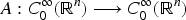
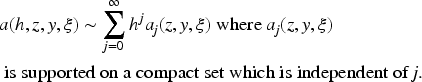
We define a very special class of semiclassical pseudodifferential operators and refer the reader to Martinez (2002) and Zworski (2012) for much deeper discussions about such operators. We say that
$A : C_{0}^{\infty} (R^{n}) ⟶ C_{0}^{\infty} (R^{n})$
is a semiclassical pseudodifferential operator if
$A (z, h D) u (z) = \frac{1}{(2 π h)^{n}} \int_{R^{n}} \int_{R^{n}} e^{\frac{i}{h} ⟨ z - y, ξ ⟩} a (h, z, y, ξ) u (y) d y d ξ,$
(7.6)
such that
$\begin{aligned} a (h, z, y, ξ) \sim \sum_{j = 0}^{\infty} h^{j} a_{j} (z, y, ξ) where a_{j} (z, y, ξ) \\ is supported on a compact set which is independent of j . \end{aligned}$
In what follows we will say that
$A (z, h D) = A_{0} (z, h D) + O (h^{k}),$
if there exists a semiclassical pseudodifferential operator $B (x, h D)$ such that
$A (z, h D) = A_{0} (z, h D) + h^{k} B (z, h D),$
We use $O (h^{\infty})$ when this is true for every $k$ . Using that
$\begin{aligned} a_{j} (z, y, ξ) \sim \sum_{α \in N} \frac{1}{α!} \partial_{x}^{α} a_{j} (z, z, ξ) (z - y)^{α} and \\ (z - y)^{α} e^{\frac{i}{h} ⟨ z - y, ξ ⟩} = (h D_{ξ})^{α} e^{\frac{i}{h} ⟨ z - y, ξ ⟩}, \end{aligned}$
one can use and Borel summation formula to show that if $A (z, h D)$ is defined as in (7.6), then
$\begin{aligned} A (z, h D) u (z) = \frac{1}{(2 π h)^{n}} \int_{R^{n}} \int_{R^{n}} e^{\frac{i}{h} ⟨ z - y, ξ ⟩} \tilde{a} (h, z, ξ) u (y) d y d ξ + O (h^{\infty}), where \\ \tilde{a} (h, z, ξ) \sim \sum_{j = 0}^{\infty} h^{j} {\tilde{a}}_{j} (z, ξ), for some {\tilde{a}}_{j} (z, ξ) \in C_{0}^{\infty}, with support independent of j \\ and {\tilde{a}}_{0} (z, ξ) = a_{0} (z, z, ξ) is defined to be the (left) principal symbol of A (x, h D) . \end{aligned}$
We can define semiclassical pseudodifferential operators on a manifold by using local coordinates, see for example Zworski (2012). If $M$ is a $C^{\infty}$ manifold, ${U_{μ}}$ , $U_{μ} \subset M$ form an open cover of $M$ and $Ψ_{μ} : U_{μ} ⟼ R^{n}$ , are local charts and ${χ_{μ}}$ is a partition of unity subordinated to ${U_{μ}}$ , then $P$ is a semiclassical pseudodifferential operator on $M$ if for $f \in C^{\infty} (M)$ ,
$\begin{aligned} χ_{μ} P χ_{ν} f = O (h^{\infty}), provided supp χ_{μ} \cap supp χ_{ν} = \emptyset, otherwise \\ (χ_{μ} P χ_{ν} f) (Ψ_{μ}^{- 1} (z)) = \frac{1}{(2 π h)^{n}} \int_{R^{n}} e^{- \frac{i}{h} ⟨ z - y, ξ ⟩} χ_{μ} (Ψ_{μ}^{- 1} (z)) a_{μ, ν} (h, z, ξ) (χ_{ν} f) (Ψ_{μ}^{- 1} (y)) d y d ξ, \\ with a_{μ, ν} (h, z, ξ) \sim \sum_{j = 0}^{\infty} h^{j} a_{j, μ, ν} (z, ξ), with a_{j, μ, ν} with compact supported independent of j \end{aligned}$
(7.7)
and this characterization is independent of the atlas ${(U_{μ}, Ψ_{μ})}$ , see for example Section 14.2 of Zworski (2012).

We want to show that $\frac{1}{h} U_{V} (\frac{n}{2} + \frac{i}{h})$ fits this definition. A similar discussion for regular pseudodifferential operators is carried out in Section 12 of Chapter 0 of Yafaev (2010). We already know it satisfies the first part of (7.7), and we need to check it satisfies the second part. For fixed $ω \in S^{n}$ , let $Π (ω)$ be the plane orthogonal to $ω$ passing through the origin:
$Π (ω) = {ξ \in R^{n + 1} : ⟨ ξ, ω ⟩ = 0},$
and let
$Ω_{ω} = {θ \in S^{n} : | θ - ω | < \frac{1}{2}}$
and let $Ψ_{ω} : Ω_{ω} ⟼ U_{ω}$ denote the orthogonal projection of $S^{n}$ onto $Π (ω)$ restricted to $Ω_{ω}$ . For each fixed $ω,$ its inverse is given by
$\begin{aligned} Ψ_{ω}^{- 1} : U_{ω} ⟼ Ω_{ω} \\ Ψ_{ω}^{- 1} (y) = y + (1 - | y |^{2})^{\frac{1}{2}} ω . \end{aligned}$
This collection ${(Ω_{ω}, Ψ_{ω}), ω \in S^{n}}$ gives an atlas of $S^{n}$ . Of course one just needs finitely many $ω \in S^{n}$ to produce form an atlas.

In our case we have an operator of the form
$\begin{aligned} (A (θ, h D) f) (θ) & = \frac{1}{(2 π h)^{n}} \int_{S^{n}} \int_{Π (θ)} e^{\frac{i}{h} ⟨ ξ, θ - θ^{'} ⟩} a (h, θ, ξ) f (θ^{'}) d μ_{θ} (ξ) d θ^{'}, \\ with a (h, θ, ξ) & \sim \sum_{j = 0}^{\infty} h^{j} a_{j} (θ, ξ), a_{j} \in C_{0}^{\infty}, \end{aligned}$
and we want to show that for each fixed $ω \in S^{n}$ , $(χ A (θ, h D) χ f) (Ψ_{ω}^{- 1})$ is given by a formula as in (7.7). In fact we just need to verify that this is the case if $θ = ω$ . Indeed, if $T = T_{ω, θ}$ is the orthogonal transformation such that $θ = T ω$ , and if we define $θ^{'} = T ω^{'}$ , one can check that
$(A (T ω, h D) f) (T ω) = \frac{1}{(2 π h)^{n}} \int_{S^{n}} \int_{Π (ω)} e^{\frac{i}{h} ⟨ ξ, w - w^{'} ⟩} a (h, T ω, T ξ) f (T w^{'}) d μ_{ω} (ξ) d ω^{'} .$
So we just need to consider the case $ω = θ$ and verify that $(χ A (θ, h D) χ f) (Ψ_{θ}^{- 1})$ is given by a formula as in (7.7). We set $z = Ψ_{θ} (θ)$ (we are just shifting the origin in $Π (θ)$ to $z$ instead of $0$ ) and $y = Ψ_{θ} (θ^{'}),$ and $χ \in C^{\infty} (S^{n})$ supported near $θ,$ then $θ^{'} = Ψ_{θ}^{- 1} (y) = y + (1 - | z - y |^{2})^{\frac{1}{2}} θ$ , and since $⟨ ξ, θ ⟩ = 0$ for $ξ \in Π (θ),$
$\begin{aligned} (χ A (θ, h D) χ f) (Ψ_{θ}^{- 1} (z)) \\ = \frac{1}{(2 π h)^{n}} \int_{Π_{θ}} \int_{Π_{θ}} e^{\frac{i}{h} ⟨ z - y, ξ ⟩} χ (Ψ_{θ}^{- 1} (z)) a (h, Ψ_{θ}^{- 1} (z), ξ) (χ f) (Ψ_{θ}^{- 1} (y)) \frac{1}{\sqrt{1 - | y - z |^{2}}} d μ_{θ} (ξ) d μ_{θ} (y) . \end{aligned}$
Here we used that $\frac{1}{\sqrt{1 - | y - z |^{2}}} d y = d θ^{'} .$ If we proceed as above we can see that the integral decays is of order $O (h^{\infty})$ if $| z - y | > δ > 0,$ and so we may expand
$\frac{1}{\sqrt{1 - | y - z |^{2}}} = 1 + \sum_{j = 0}^{\infty} C_{j} | z - y |^{2 j}, for | z - y | < ε,$
and use that $| z - y |^{2} e^{\frac{i}{h} ⟨ z - y, ξ ⟩} = h^{2} Δ_{ξ} e^{\frac{i}{h} ⟨ z - y, ξ ⟩}$ and integrate by parts in $ξ$ , we find that
$\begin{aligned} (χ A (θ, h D) χ f) (Ψ_{θ}^{- 1} (z)) = \frac{1}{(2 π h)^{n}} \int_{R^{n}} \int_{R^{n}} e^{\frac{i}{h} ⟨ z - y, ξ ⟩} b (h, z, ξ) (χ f) (Ψ_{θ}^{- 1} (y)) d ξ d y + O (h^{\infty}), \\ where b (h, z, ξ) \sim a_{0} (Ψ_{θ}^{- 1} (z), ξ) + \sum_{j = 1}^{\infty} h^{j} b_{j} (z, ξ), b_{j} \in C_{0}^{\infty}, \end{aligned}$
and we are just using $d ξ = d μ_{θ} (ξ)$ and $d y = d μ_{θ} (y)$ . In our case $a_{0} (Ψ_{θ}^{- 1} (z), ξ) = H (θ, ξ)$ , defined in (7.5) and (4.2). Notice that any other operator $\tilde{A}$ of the same type such that
$\tilde{b} (h, Ψ_{θ}^{- 1} (z), ξ) \sim H (θ, ξ) + \sum_{j = 1}^{\infty} h^{j} {\tilde{b}}_{j} (θ, ξ), {\tilde{b}}_{j} \in C_{0}^{\infty},$
will satisfy $A - \tilde{A} = O (h),$ and so we say that $H (θ, ξ)$ is the principal symbol of $A (θ, h D)$ , and this proves the following Theorem 7.4
If $V \in C_{0}^{\infty} (B^{n + 1})$ , the operator $\frac{1}{h} U_{V} (\frac{n}{2} + \frac{i}{h})$ defined in (6.5) is a semiclassical pseudodifferential operator on $S^{n}$ and its principal symbol is equal to $H (θ, ξ) = - 2^{n - 1} X (V) (\frac{ξ}{2}, θ)$ .

8. The Proof of Theorem 2.1 for $V \in C_{0}^{\infty} (H^{n + 1})$

We first prove Theorem 2.1 for $V \in C_{0}^{\infty} (H^{n + 1})$ and for polynomials $f (t)$ and then use the Stone–Weiestrass theorem to extend it to compactly supported functions. As already mentioned in Section 3, the idea of using the Stone–Weiestrass theorem in this context is not new. In the next section we extend the result for $V \in x^{m} L^{\infty} (H^{n + 1})$ , $m > 1$ .

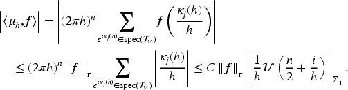
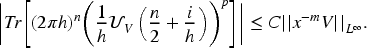
If $V \in C_{0}^{\infty} (H^{n + 1})$ , we have shown that $(1 / h) U_{V} (\frac{n}{2} + \frac{i}{h})$ is a semiclassical pseudodifferential operator whose principal symbol is $- 2^{n - 1} X (V) (\frac{ξ}{2}, θ)$ . The calculus of semiclassical pseudodifferential operator, see Martinez (2002) and Zworski (2012) and Theorem 7.4 give that for any $p \in N$ , ${(\frac{1}{h} U_{V} (h))}^{p}$ satisfies

\begin{aligned} {(\frac{1}{h} U_{V} (\frac{n}{2} + \frac{i}{h}))}^{p} (θ, θ^{'}) = \frac{1}{(2 π h)^{n}} \int_{Π (θ)} e^{- \frac{i}{h} ⟨ ξ, θ - θ^{'} ⟩} {(- 2^{n - 1} X (V) (\frac{ξ}{2}, θ))}^{p} d μ_{θ} (ξ) \\ + \frac{h}{(2 π h)^{n}} \int_{Π (θ)} e^{- \frac{i}{h} ⟨ ξ, θ - θ^{'} ⟩} b (h, θ, ξ) d ξ + O (h^{\infty}), b (h, θ, ξ) \sim \sum_{j = 0}^{\infty} h^{j} b_{j} (θ, ξ) . \end{aligned}

and therefore its trace satisfies

\begin{aligned} (2 π h)^{n} T r {(\frac{1}{h} U_{V} (\frac{n}{2} + \frac{i}{h}))}^{p} = \int_{S^{n}} (2 π h)^{n} {(\frac{1}{h} U_{V} (\frac{n}{2} + \frac{i}{h} h))}^{p} (θ, θ) d θ + O (h) \\ = \int_{S^{n}} \int_{Π (θ)} {(- 2^{n - 1} X (V) (\frac{ξ}{2}, θ))}^{p} d μ_{θ} (ξ) d θ + O (h) = \int_{R} t^{p} d ν (t) + O (h) . \end{aligned}

(8.1)

where

ν

is the measure defined in (2.10).

Since $V \in x^{m} L^{\infty} (H^{n + 1})$ for all $m$ , it follows from (6.34) and (8.1) that for $p \geq 1$ ,

(2 π h)^{n} \sum_{e^{i δ (s)} \in spec T_{V}} {(\frac{1}{h} κ_{j} (h))}^{p} - \int_{R} t^{p} d ν (t) = O (h), δ_{j} (\frac{n}{2} + \frac{i}{h}) = κ_{j} (h) .

(8.2)

This proves Theorem 2.1 if $V \in C_{0}^{\infty} (H^{n + 1})$ , $f (t) = t^{p}$ , with $p \in N$ , $p \geq 1$ . To prove the result for $f$ such that $\frac{f (t)}{t} \in C_{0} (R)$ , we appeal to the Stone-Weierstrass theorem. Since $V \in C_{0}^{\infty} (H^{n + 1})$ , $X (V) (\frac{ξ}{2}, θ) = 0$ for $| ξ |$ large and so the measure $ν$ is supported on $[- R, R]$ for some $R > 0$ . Similarly, in view of (6.4), $\frac{1}{h} κ_{j} (h) \in [- R, R]$ , for $h$ small, for all $j$ . So we may work with $f$ supported in $[- R, R]$ . Define the space

\begin{aligned} Γ ([- R, R]) = {f \in C^{0} ([- R, R]) : \frac{f (t)}{t} is continuous}, \\ equipped with the norm | | f | |_{_{Γ}} = sup_{x \in [- R, R]} | \frac{f (t)}{t} | . \end{aligned}

Since

V

is compactly supported, we can take

p = 1

in (6.29), and so if

μ_{h}

is the measure defined in (2.7), then

\begin{aligned} | ⟨ μ_{h}, f ⟩ | = | (2 π h)^{n} \sum_{e^{i κ_{j} (h)} \in spec (T_{V})} f (\frac{κ_{j} (h)}{h}) | \\ \leq (2 π h)^{n} | | f | |_{_{Γ}} \sum_{e^{i κ_{j} (h)} \in spec (T_{V})} | \frac{κ_{j} (h)}{h} | \leq C {‖ f ‖}_{_{Γ}} {‖ \frac{1}{h} U (\frac{n}{2} + \frac{i}{h}) ‖}_{Σ_{1}} . \end{aligned}

Since

\frac{f (t)}{t}

is continuous, for any

ε > 0

, there exists a polynomial

q (t)

such that

| \frac{f (t)}{t} - q (t) | < ε

, for all

t

, and so

| \frac{f (t) - t q (t)}{t} | < ε

for all t, and we conclude that the space of polynomials

q (t)

such that

q (0) = 0

is dense in

Γ ([- R, R])

. But the argument used above implies that if

q

is a such a polynomial, then

| ⟨ μ_{h}, f - q ⟩ | \leq C | | f - q | |_{_{Γ}} .

This implies that

| ⟨ μ_{h}, f ⟩ - \int_{R} q (t) d ν (t) - O (h) | \leq C | | f - q | |_{_{Γ}} .

If we first take the limit as

h \to 0

and then take a sequence of polynomials

q_{j}

, which converge to

f

Γ ([- R, R])

and the result follows.

9. The Proof of the General Case of Theorem 2.1

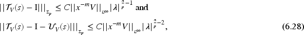
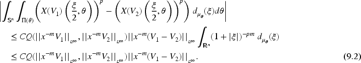
We have proved Theorem 2.1 for $V \in C_{0}^{\infty} (H^{n + 1})$ and we want to extend it to include the cases where $V \in x^{m} L^{\infty} (H^{n + 1})$ , for some $m \in (1, \infty)$ . We know from (6.27) that if $V \in x^{m} L^{\infty} (H^{n + 1})$ and $p \in N$ is such that $p \geq 1$ and $p > \frac{2 (n - \frac{1}{2})}{m - 1}$ , ${(\frac{1}{h} U_{V} (\frac{n}{2} + \frac{1}{h}))}^{p}$ is trace class and

| T r [(2 π h)^{n} (\frac{1}{h} U_{V} (\frac{n}{2} + \frac{i}{h}))^{p}] | \leq C | | x^{- m} V | |_{L^{\infty}} .

We also know from (6.32) and (6.33) that if

V_{j} \in x^{m} L^{\infty} (H^{n + 1})

, and

A_{j} = \frac{1}{h} U_{V_{j}} (\frac{n}{2} + \frac{i}{h})

j = 1, 2

, that

| T r (A_{1}^{p} - A_{2}^{p}) | \leq \sum_{j = 0}^{p - 1} | | A_{1} | |_{Σ_{p}}^{j} | | A_{1} - A_{2} | |_{Σ_{p}} | | A_{2} | |_{Σ_{p}}^{p - j - 1}

and so it follows from (6.27) that

h^{n} | T r (A_{1}^{p} - A_{2}^{p}) | \leq C | | x^{- m} (V_{1} - V_{2}) | |_{_{L^{\infty}}} \sum_{j = 0}^{p} | | x^{- m} V_{1} | |_{_{L^{\infty}}}^{j} | | x^{- m} V_{2} | |_{_{L^{\infty}}}^{p - j - 1} .

(9.1)

On the other hand,

\begin{aligned} \int_{S^{n}} \int_{Π (θ)} (X (V_{1}) (\frac{ξ}{2}, θ))^{p} - (X (V_{2}) (\frac{ξ}{2}, θ))^{p}) d_{μ_{θ}} (ξ) d θ \\ = \int_{S^{n}} \int_{Π (θ)} ((X (V_{1}) (\frac{ξ}{2}, θ) - X (V_{2}) (\frac{ξ}{2}, θ)) Q (X (V_{1}) (\frac{ξ}{2}, θ), X (V_{2}) (\frac{ξ}{2}, θ)) d_{μ_{θ}} (ξ) d θ, \end{aligned}

where

Q (x, y)

is a homogeneous polynomial of degree

p - 1

. Therefore, in view of (4.3) and (4.4), we obtain

\begin{aligned} | \int_{S^{n}} \int_{Π (θ)} (X (V_{1}) (\frac{ξ}{2}, θ))^{p} - (X (V_{2}) (\frac{ξ}{2}, θ))^{p}) d_{μ_{θ}} (ξ) d θ | \\ \leq C Q (| | x^{- m} V_{1} | |_{_{L^{\infty}}}, | | x^{- m} V_{2} | |_{_{L^{\infty}}}) | | x^{- m} (V_{1} - V_{2}) | |_{_{L^{\infty}}} \int_{R^{n}} (1 + | ξ |)^{- p m} d_{μ_{θ}} (ξ) \\ \leq C Q (| | x^{- m} V_{1} | |_{_{L^{\infty}}}, | | x^{- m} V_{2} | |_{_{L^{\infty}}}) | | x^{- m} (V_{1} - V_{2}) | |_{_{L^{\infty}}} . \end{aligned}

(9.2)

Therefore, (9.1) and (9.2) imply that (8.1) also holds for

V \in Z_{0, m} := \bar{C_{0}^{\infty} (H^{n + 1})}

, which is defined to be the closure of

C_{0}^{\infty} (H^{n + 1})

with the topology of

x^{m} L^{\infty}

, provided

p > \frac{2 (n - \frac{1}{2})}{m - 1}

One has that

x^{m} L^{\infty} (H^{n + 1}) \subset x^{m^{'}} L^{\infty} (H^{n + 1}), provided m \geq m^{'},

but in fact one also has

x^{m} L^{\infty} (H^{n + 1}) \subset Z_{0, m^{'}}, provided m > m^{'} .

To see that, notice that if

V \in x^{m} L^{\infty} (H^{n + 1})

and

χ_{k} (w) = 1

| w | < 1 - \frac{1}{k}

and

χ_{k} (w) = 0

| w | > 1 - \frac{1}{2 k}

, then

\begin{aligned} | | x^{m^{'}} (V - χ_{k} V) | | & = | | x^{- m} V x^{m - m^{'}} (1 - χ_{k}) | |_{\leq} | | x^{- m} V | |_{_{L^{\infty}}} | | x^{m - m^{'}} (1 - χ_{k} (w)) | |_{_{L^{\infty}}} \\ \leq | | x^{- m} V | |_{_{L^{\infty}}} k^{m^{'} - m} \to 0 as k \to \infty . \end{aligned}

This means that

χ_{k} V \to V

x^{m^{'}} L^{\infty} (H^{n + 1})

, if

m^{'} < m

. So, if

p > \frac{2 (n - \frac{1}{2})}{m - 1}

, pick

m^{'} \in (1, m)

such that

p > \frac{2 (n - \frac{1}{2})}{m^{'} - 1}

, and so the result holds for

Z_{0, m^{'}} \supset x^{m} L^{\infty} (H^{n + 1})

. This implies that Theorem 2.1 holds for polynomials of degree

p > \frac{2 (n - \frac{1}{2})}{m - 1}

. We modify the proof of the case

V \in C_{0}^{\infty} (H^{n + 1})

, and we use space

Γ_{p} ([- R, R])

, where

\frac{f (t)}{t^{p}}

is continuous, the argument goes through and we prove (2.9) for continuous functions

f

which vanish to order

p

at zero.

10. The Proof of Theorem 2.2

If $V (w) = V (ρ (w))$ , where $ρ (w) = d_{g_{0}} (w, 0) = \log (\frac{1 + | w |}{1 - | w |})$ , it follows from (4.2) that

\begin{aligned} - 2^{n - 1} X_{V} (t, ξ) & = G_{V} (r) = \int_{- \infty}^{- \frac{1}{2}} V (T (r, t)) \frac{1}{1 + 2 t} d t, where \\ r = | ξ |, T (r, t) & = \log (\frac{1 + A (t, r)}{1 - A (t, r)}) and A (t, r) = {[\frac{(1 + t)^{2} + r^{2}}{t^{2} + r^{2}}]}^{\frac{1}{2}} . \end{aligned}

(10.1)

Notice that $x = (1 - | w |) / (1 + | w |) = e^{- d_{g_{0}} (w, 0)}$ , defined in (2.3), and so if $V \in x^{m} L^{\infty},$ for all $m > 0$ , implies that $e^{m d_{g_{0}} (w, 0)} V (w) \in L^{\infty}$ for all $m$ , and so $V$ is super-exponentially decaying with respect to the distance function to the origin. Therefore

G_{V}^{'} (r) = - \int_{- \infty}^{- \frac{1}{2}} 4 r V^{'} (T (r, t)) \frac{1}{A (1 - A^{2})} d t .

So, if

\pm V^{'} (ρ) \geq 0

for all

ρ

, then

\mp G_{V}^{'} (r) \geq 0

for all

r

. Also notice that

G_{V}^{'} (r) = 0

for all

r \geq r_{0}

if and only if

V^{'} (T (r, t)) = 0

for all

r \geq r_{0}

and all

t \in (- \infty, - \frac{1}{2})

. But since

T (r, t) = d_{g_{0}} (w, 0)

with

w = θ + \frac{t θ + ξ}{t^{2} + | ξ |^{2}}

, this implies that

V^{'} (ρ) = 0

for all points

w \in H^{n + 1}

such that

d_{g_{0}} (w, 0) \geq r_{0} .

But if

V (ρ) \to 0

r \to 1,

it follows that

V (ρ) = 0

for

ρ \geq r_{0} .

So we conclude that if

V^{'} (ρ) \neq 0

V (r) \neq 0,

the same is true for

G_{V} (r) .

So we may just assume that $V (ρ)$ nonpositive and increasing and therefore $G_{V} (r)$ is nonnegative and decreasing. If we have two potentials $V_{1} (ρ)$ and $V_{2} (ρ)$ for which (2.12) holds, then

meas ((G_{V_{1}})^{- 1} (α, β)) = meas ((G_{V_{2}})^{- 1} (α, β)) for all (α, β) \subset (0, \infty) .

(10.2)

In particular, we must have

A := G_{V_{1}} (0) = G_{V_{2}} (0) \neq 0

. Otherwise, say for example that

G_{V_{1}} (0) > G_{V_{2}} (0) > 0

, since the functions are decreasing, there would be an interval

(α, β) \subset (G_{V_{2}} (0), G_{V_{1}} (0))

that would violate (10.2). If

G_{V_{1}} (0) = G_{V_{2}} (0) = 0

, since the functions are decreasing,

G_{V_{1}} (r) = G_{V_{2}} (r) = 0

for all

r > 0

. But in that case the injectivity of the

X

-ray transform for super-exponentially decaying potentials, see Corollary 1.3 of Chapter 3 of Helgason (1999), implies that

V_{1} = V_{2} = 0

, which certainly is not the case.

Also, if $G_{V_{1}} (r) = 0$ for all $r \geq R,$ then

lim_{ε \to 0} meas (G_{V_{1}}^{- 1} (ε, A - ε)) = lim_{ε \to 0} (G_{V_{1}}^{- 1} (A - ε) - G_{V_{1}}^{- 1} (ε)) = R .

Since the same would have to be true for

G_{V_{2}}

, then

G_{V_{2}} (R) = 0

and so

G_{V_{2}} (r) = 0

for all

r \geq R

. So we conclude that we either have

\begin{aligned} G_{V_{j}} : [0, R] ⟶ [0, A], j = 1, 2, or \\ G_{V_{j}} : [0, \infty) ⟶ (0, A], j = 1, 2. \end{aligned}

In either case the functions are injective and the closure of their ranges are the same. So we may define

ψ (r) = (G_{V_{1}})^{- 1} (G_{V_{2}} (r)) .

But (10.2) implies that if

α < β

and

\begin{aligned} α = G_{V_{1}} (a_{1}), β = G_{V_{1}} (b_{1}), a_{1} < b_{1}, \\ α = G_{V_{2}} (a_{2}), β = G_{V_{2}} (b_{2}), a_{2} < b_{2}, \end{aligned}

then

a_{2} - b_{2} = a_{1} - b_{1}

, and so

\frac{G_{V_{1}} (b_{1}) - G_{V_{1}} (a_{1})}{b_{1} - a_{1}} = \frac{G_{V_{2}} (b_{2}) - G_{V_{2}} (a_{2})}{b_{2} - a_{2}} .

and we deduce that, for every

a_{j} > 0

j = 1, 2

, such that

G_{V_{1}} (a_{1}) = G_{V_{2}} (a_{2})

, we have

G_{V_{1}}^{'} (a_{1}) = G_{V_{2}}^{'} (a_{2})

, and this implies that

ψ^{'} (α) = 1

, but since

α

is arbitrary,

ψ^{'} (r) = 1

, but we know that

ψ (0) = 0

and so

ψ (r) = r

This implies that $G_{V_{1}} (r) = G_{V_{2}} (r)$ , for all $r > 0$ . Again, the injectivity of the $X$ -ray transform for this class of potentials implies that $V_{1} = V_{2}$ .

Footnotes

Acknowledgments

The author is very grateful to an anonymous referee for carefully reading the article, making many suggestions on how to improve the exposition and for insisting that more details should be provided.

Funding

The authors disclosed receipt of the following financial support for the research, authorship, and/or publication of this article: The author was funded by the Simons Foundation grant #848410.

Declaration of Conflicting Interests

The author declared no potential conflicts of interest with respect to the research, authorship, and/or publication of this article.

References

Abramowitz

Stegun

(1972). Handbook of mathematical functions with formulas, graphs, and mathematical tables. Dover.

Bargmann

(1949). On the connection between phase shifts and scattering potential. Reviews of Modern Physics, 21(3), 488–493.

Berry

M. V.

(1966). Semi-classical scattering phase shifts in the presence of metastable states. Proceedings of the Physical Society of London, 88(2), 285–292.

Birman

M. S.

Yafaev

D. R.

(1980). Asymptotics of the spectrum of the s-matrix in potential scattering. Soviet Physics. Doklady, 25, 989–990.

Birman

M. S.

Yafaev

D. R.

(1982). Asymptotic behavior of limit phases for scattering by potentials without spherical symmetry. Theoretical and Mathematical Physics, 51, 344–350.

Borthwick

(2010). Sharp upper bounds on resonances for perturbations of hyperbolic space. Asymptotic Analysis, 69, 45–85.

Borthwick

Crompton

(2014). Resonance asymptotics for Schrödinger operators on hyperbolic space. Journal of Spectral Theory, 4(3), 515–567.

Borthwick

Wang

(2024). Existence of resonances for Schrodinger operators on hyperbolic space. Annals of PDE, 17(6), 2077–2108.

Bouclet

J.-M.

(2013). Absence of eigenvalue at the bottom of the continuous spectrum on asymptotically hyperbolic manifolds. Annals of Global Analysis and Geometry, 44(2), 115–136.

10.

Bulger

Pushnitski

(2012). The spectral density of the scattering matrix for high energies. Communications in Mathematical Physics, 316, 693–704.

11.

Bulger

Pushnitski

(2013). The spectral density of the scattering matrix of the magnetic Schrödinger operator for high energies. Journal of Spectral Theory, 3, 517–534.

12.

Chen

Hassell

(2016). Resolvent and spectral measure on non-trapping asymptotically hyperbolic manifolds I: Resolvent construction at high energy. Communications in Partial Differential Equations, 41(3), 515–578.

13.

Christiansen

Uribe

(2021). The semiclassical structure of the scattering matrix for a manifold with infinite cylindrical end. arXiv:2112.12007.

14.

Datchev

Gell-Redman

Hassell

Humphries

(2014). Approximation and equidistribution of phase shifts: Spherical symmetry. Communications in Mathematical Physics, 326, 209–236.

15.

Duistermaat

J. J.

(1974). Oscillatory integrals, Lagrange immersions and unfolding of singularities. Communications on Pure and Applied Mathematics, 27, 207–281.

16.

B. C.

(1968). Method of calculating phase shifts for spherically symmetric potentials. Chemical Physics, 48, 2852. https://doi.org/10.1063/1.1669542

17.

Fefferman

Graham

(1985). Conformal invariants. The mathematical heritage of élie Cartan (Lyon, 1984). Astérisque, 1985, Numero Hors Serie, 95–116.

18.

Gell-Redman

Hassell

(2012). Potential scattering and the continuity of phase shifts. Mathematical Research Letters, 19(03), 719–729.

19.

Gell-Redman

Hassell

(2020). The distribution of phase shifts for semiclassical potentials with polynomial decay. International Mathematics Research Notices, 2020(19), 6294–6346.

20.

Gell-Redman

Hassell

Zelditch

(2015). Equidistribution of phase shifts in semiclassical potential scattering. Journal of the London Mathematical Society, 91(1), 159–179.

21.

Gell-Redman

Ingremeau

(2019). Equidistribution of phase shifts in obstacle scattering. Communications in Partial Differential Equations, 44(1), 1–19.

22.

Goh'berg

I. C.

Krein

M. G.

(1969). Introduction to the theory of linear nonselfadjoint operators. Translations of Mathematical Monographs (Vol. 18.) American Mathematical Society.

23.

Graham

C. R.

(2000). Volume and area renormalization for conformally compact Einstein metrics. Rendiconti del Circolo Matematico di Palermo, 1(Suppl. 63), 31–42.

24.

Guillarmou

(2005). Absence of resonances near the critical line on asymptotically hyperbolic spaces. Asymptotic Analysis, 42(1-2), 105–121.

25.

Guillemin

Sternberg

(2013). Semi-classical analysis. International Press. xxiv+446 pp. ISBN:978-1-57146-276-3.

26.

Guillopé

(1992). Fonctions zêta de Selberg et surfaces de géométrie finie. In Zeta functions in geometry (Tokyo, 1990), advanced studies in pure mathematics (Vol. 21, pp. 33–70). Kinokuniya, Tokyo.

27.

Guillopé

Zworski

(1995). Polynomial bounds on the number of resonances for some complete spaces of constant negative curvature near infinity. Asymptotic Analysis, 11, 1–22.

28.

Helgason

(1999). The Radon transform (2nd ed.) Progr. Math. 5. Birkhäuser.

29.

Hörmander

(1994). The analysis of linear partial differential operators (Vol. IV). Springer-Verlag.

30.

Ingremeau

(2018). Equidistribution of phase shifts in trapped scattering. Journal of Spectral Theory, 8(4), 1199–1220.

31.

Isozaki

Kurylev

(2014). Introduction to Spectral Theory and Inverse Problem on Asymptotically Hyperbolic Manifolds MSJ memoirs, 32. Mathematical Society of Japan.

32.

Itoh

Satoh

(2013). Horospheres and hyperbolic spaces. Kyushu Journal of Mathematics, 67(2), 309–326.

33.

Joshi

Sá Barreto

(2000). Inverse scattering on asymptotically hyperbolic manifolds. Acta Mathematica, 184, 41–86.

34.

Kostas

Andersson

(2001). Scattering of scalar waves by rotating black holes. Classical and Quantum Gravity, 18, 1939–1966.

35.

Kuipers

Niederreiter

(1974). Uniform distribution of sequences. Wiley Interscience [John Wiley & Sons].

36.

Lafontaine

(2015). An introduction to differential nanifolds (2nd ed.). Springer. xx+395. https://doi.org/10.1007/978-3-319-20735-3

37.

Landau

L. D.

Lifshitz

E. M.

(1965). Quantum mechanics: Nonrelativistic theory. Pergamon Press.

38.

Lax

(2001). The Radon transform and translation representation. Journal of Evolution Equations, 1, 311–323.

39.

Lax

P. D.

Phillips

R. S.

(1976). Scattering theory for automorphic functions. Annals of mathematics studies no. 87. Princeton Univ. Press.

40.

Lax

P. D.

Phillips

R. S.

(1979). Translation representations for the solution of the non-Euclidean wave equation. Communications on Pure and Applied Mathematics, 32, 617–667.

41.

Lax

P. D.

Phillips

R. S.

(1980). Translation representations for the solution of the non-Euclidean wave equation. Communications on Pure and Applied Mathematics, 33, 685.

42.

Levinson

(1949). On the uniqueness of the potential in a Schrödinger equation for a given asymptotic phase. Matematisk-fysiske Meddelelser / Det Kongelige Danske Videnskabernes Selskab, 25(9), 29.

43.

Martinez

(2002). An introduction to semiclassical and microlocal analysis. Universitext Springer-Verlag. viii+190 pp. ISBN: 0-387-95344-2.

44.

Mazzeo

(1991). Unique continuation at infinity and embedded eigenvalues for asymptotically hyperbolic manifolds. American Journal of Mathematics, 113, 25–45.

45.

Mazzeo

Melrose

(1987). Meromorphic extension of the resolvent on complete spaces with asymptotically constant negative curvature. Journal of Functional Analysis, 75(2), 260–310.

46.

McKean

H. P.

(1970). An upper bound to the spectrum of

Δ

on a manifold of negative curvature. Journal of Differential Geometry, 4(3), 359–366.

47.

Melrose

(1995). Geometric scattering theory. Cambridge University Press.

48.

Melrose

Sá Barreto

Vasy

(2014). Analytic continuation and semiclassical resolvent estimates on asymptotically hyperbolic spaces. Communications in Partial Differential Equations, 39(3), 452–511.

49.

Nakamura

(2016). Microlocal properties of scattering matrices. Communications in Partial Differential Equations, 41(6), 894–912. https://doi.org/10.1080/03605302.2016.1167082

50.

Perry

(1989). The Laplace operator on a hyperbolic manifold, II. Eisenstein series and the scattering matrix. Journal für Die Reine und Angewandte Mathematik, 398, 67–91.

51.

Piel

Chrysos

(2020). From Lippmann–Schwinger formulations to a general formula for absolute asymptotic scattering phase functions and shifts: A unified framework for potentials of any range. Molecular Physics, 118(1), e1587024. https://doi.org/10.1080/00268976.2019.1587024

52.

Sá Barreto

(2005). Radiation fields, scattering and inverse scattering on asymptotically hyperbolic manifolds. Duke Mathematical Journal, 129(3), 407–480.

53.

Sá Barreto

Wang

(2016). The semiclassical resolvent on conformally compact manifolds with variable curvature at infinity. Communications in Partial Differential Equations, 41(8), 1230–1302.

54.

Sá Barreto

Wang

(2025). The distribution of negative eigenvalues of Schrödinger operators on asymptotically hyperbolic manifolds. Journal of Spectral Theory, 15(2), 679–727.

55.

Simon

(2005). Trace ideals and their applications. Mathematical surveys and monographs (Vol. 120). American Mathematical Society.

56.

Stein

(1956). Interpolation of linear operators. Transactions of the American Mathematical Society, 83, 482–492.

57.

Tricomi

F. G.

Erdélyi

(1951). The asymptotic expansion of a ratio of gamma functions. Pacific Journal of Mathematics, 1, 133–142.

58.

Yafaev

(2010). Mathematical scattering theory. Analytic Theory. American Mathematical Society.

59.

Zelditch

(1986). Pseudo-differential analysis on hyperbolic surfaces. Journal of Functional Analysis, 68, 72–105.

60.

Zworski

(2012). Semiclassical analysis. Graduate student in mathematics 138. American Mathematical Society. xii+431 pp. ISBN: 978-0-8218-8320-4.

The High Energy Distribution of Scattering Phase Shifts of Schrödinger Operators in Hyperbolic Space

Abstract

Keywords

1. Introduction

2. The Statement of the Main Results

4. The Geodesic X -Ray Transform in H n + 1

Proposition 6.1 (Proposition 3.2 of Guillarmou, 2005)

Footnotes

Acknowledgments

Funding

Declaration of Conflicting Interests

References

4. The Geodesic $X$ -Ray Transform in $H^{n + 1}$