The goal of the paper is to provide a sequence of eigenfunctions that saturates the bounds obtained by Koch and Tataru for the multidimensional Hermite operator. More precisely, several such sequences of eigenfunctions have already been identified by Koch and Tataru, and we present an example in another range of .
Let denote the sequence of eigenspaces of the Hermite operator (also called the quantum harmonic oscillator) on with :
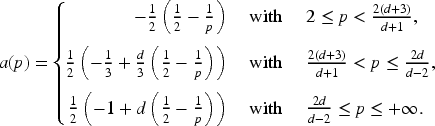
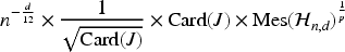
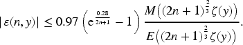
Each eigenspace is finite-dimensional (more precisely grows like as ). The classical paper by Koch and Tataru (2005) gives an almost complete set of optimal inequalities for all for the eigenspaces . The result reads as follows:
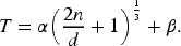
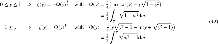
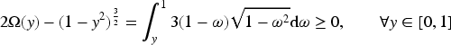
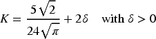
where is an explicit convex function of , defined by
Let us write a few words about the critical exponent . The following bound is shown in Koch et al. (2007) (and is probably obtainable by the arguments of Koch and Tataru (2005)):
In the remarkable paper by Jeong et al. (2024b), it is shown that the logarithmic factor is indeed unnecessary for , while the case remains open. We also refer the reader to Jeong et al. (2024a) for a related topic.
The paper by Koch and Tataru (2005) also provides proofs of sharpness of the bounds and it is interesting to see whether one could give explicit examples of sequence of eigenfunctions saturating such bounds. At the end of Koch and Tataru (2005), explicit examples are provided for
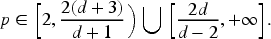
The aim of this article is to extend this analysis in the middle range .
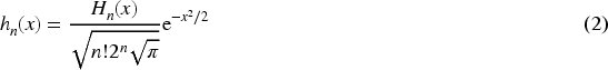
Before going into details, we introduce some notations for the one-dimensional eigenfunctions, namely Hermite functions:
where denotes the Hermite polynomial of order (physicists’ convention). For example, the ground state is given by . The following equalities are well-known:
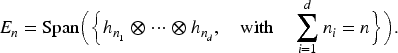
In the multidimensional case, the eigenspace (corresponding to the eigenvalue of ) can be described using a simple orthonormal basis as follows:
For the sequel, it is worthwhile to note, as at the end of Koch and Tataru (2005), that if is a non-empty set consisting of tuples satisfying , then the following function is an -normalized eigenfunction corresponding to the eigenvalue :
With such notations, we now briefly recall the known explicit examples:
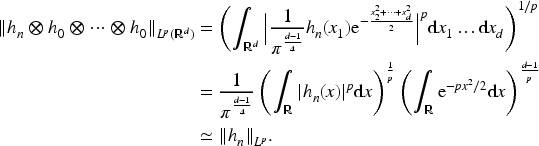
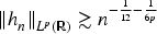
- for , the norm of the eigenfunction (which corresponds to the eigenvalue ) satisfies for :
Moreover, it is known that for (see Thangavelu, 1993, Lemma 1.5.2). This covers the relevant case since (this example is presented in Koch and Tataru (2005, Subsection 5.1)).
- for if (set if ), as shown in Koch and Tataru (2005, Subsection 5.2), one may consider a sequence of eigenfunctions of the form (4) for saturating the bounds. Another construction is given in Imekraz et al. (2016, Proposition 2.4) showing that the sequence of radial eigenfunctions of is also convenient. Geometrically, both examples concentrate around the origin.
The result of this article shows that one may also construct examples similar to (4) in the middle range .
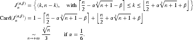
We assume . For any , and , define
and the following eigenfunction of corresponding to the eigenvalue :
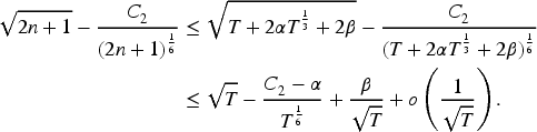
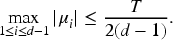
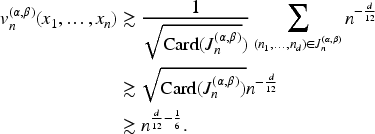
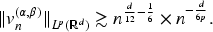
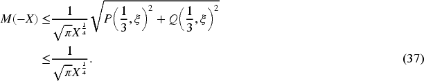
In particular, we have . Let be fixed. For any the norm saturates the Koch-Tataru estimates in the middle range:
Due to (1), the bound from below (6) is actually an equivalence for .
We finish this introduction by outlining the organization of the paper and the structure of the proof of Theorem 1.
Section 1 is devoted to giving two graphical representations in dimension that illustrate the concentration of the eigenfunctions for and . We emphasize that the parameter plays no essential role from a theoretical point of view in the statement of Theorem 1, it is only introduced to ensure for small values of in graphical representations.
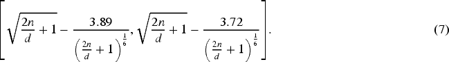
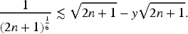
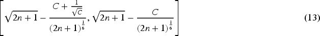
In Section 2, we prove two results (Proposition 3 and Corollary 5) that provide a quantitative statement about the spatial concentration of the one-dimensional Hermite functions . More precisely, for , Corollary 5 will imply that if then is bounded below by (up to a multiplicative constant) for belonging on the following interval
To prove such a concentration property, we use a well-known WKB approximation of the Hermite functions. More precisely, by setting
the following holds uniformly for
Written in this form, this WKB approximation of merely yields unknown constants in (7) (instead of and ) and also an unknown upper bound for the constant in Theorem 1. Without an explicit remainder in (8), the conclusion of Theorem 1 remains true for small enough, which seems essentially useless for numerical applications. To obtain the explicit condition , we need to provide an explicit constant in the remainder term of (8). This is the purpose of Proposition 2, whose proof is postponed to Section 6.
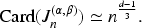
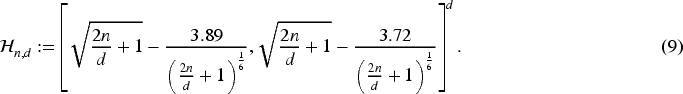
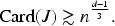
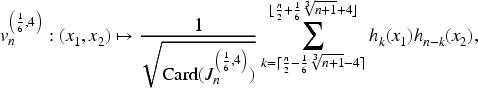
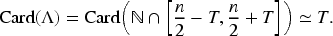
In Section 3, we give an elementary proof of the asymptotics of the cardinality of the sets for . For any choice of , Lemma 6 below ensures the following estimate
However, let us give an intuition about why this asymptotics is the good one for our purpose (the complete argument is developed in Section 4). Once we have the idea to consider an eigenfunction as (4), we search a specific set of -tuples . Due to (7), if one can ensure that each satisfies then each in (4) is bounded below by (up to a multiplicative constant) on the following hypercube
Hence, the norm of the function (4) is bounded below (up to a multiplicative constant) by
namely because the volume of the hypercube (9) is of order . In order to reach the lower bound (6), we require a bound like
Note now that each satisfies (so that (4) is an eigenfunction corresponding to ). The technical condition finally leads to the definition of in Theorem 1.
As written above, the last point is to give an explicit constant in the remainder in (8). In Section 5, we establish several explicit inequalities for the Airy functions which do not appear explicitly in the literature but can be deduced from Olver (1997). These explicit inequalities are then used in Section 6, where the constants in the analysis of Olver (1997) are followed.
In all the paper, we use the notation and the following classical notations:
for any positive numbers and , we write to mean that for some positive constant (if the exponent is relevant in and ),
means ,
means and .
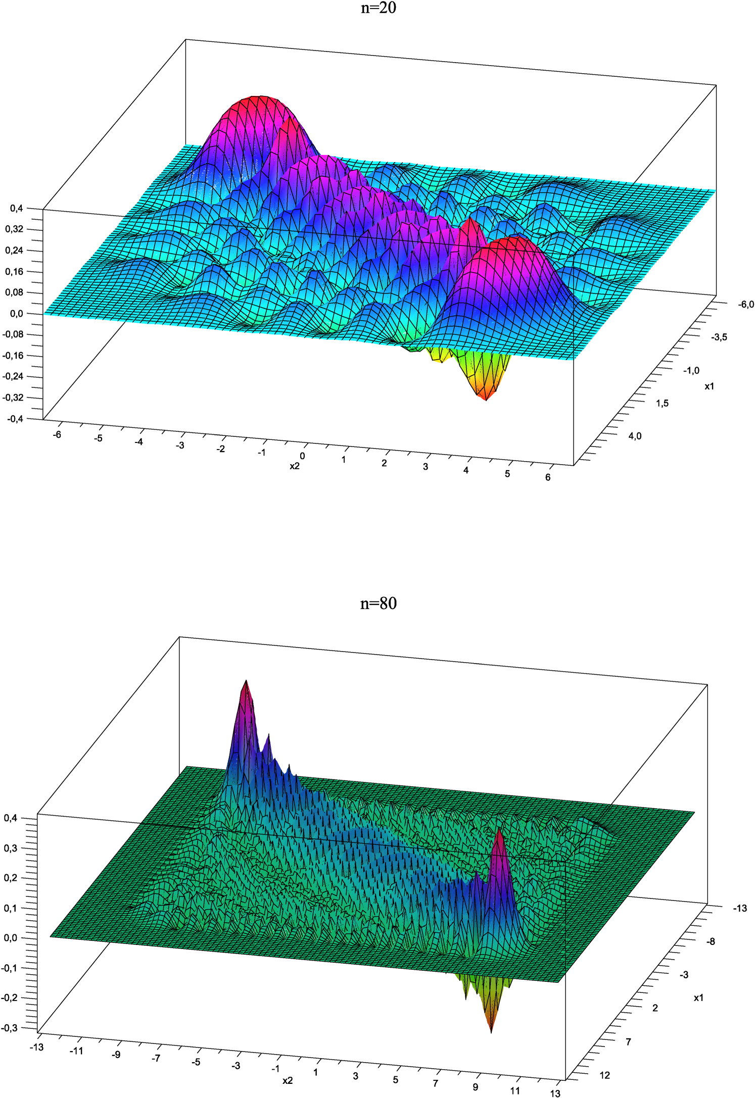
Graphical Representations in Dimension
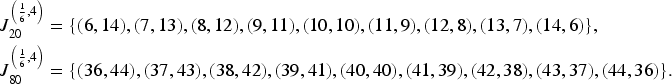
In dimension , the sets are easy to describe and we indeed have
As , the number tends to , and it appears graphically that the different eigenfunctions in (5) change signs except if lies in a concentration region. Since our choice of is somewhat restricted if we want to use (2) with factorials, and since for , we will use the extra parameter in order to make large enough to expect a cancellation phenomenon outside a concentration region. We choose , which is the maximal value allowed by Theorem 1, and that provide quite satisfactory graphical representations. Here is the formula for the eigenfunction (corresponding to the eigenvalue ):
Here are two graphical representations on for and of and we check the equalities
As mentioned in the introduction, these graphical representations confirm the concentration at least around the two points with coordinates around .
Study of the One-dimensional Eigenfunctions
For any and any positive integer , we define:
We require an explicit approximation of the one-dimensional Hermite functions in the allowed region , as stated in the following result:
For any , the following inequality holds uniformly for any :
The previous result is obtained by carefully following the constants in a standard WKB method with explicit remainders (see Section 6 for details of the proof). The simple constant has been chosen because it is sufficient for what follows1 but the proof in Section 6 provides a slightly better constant. Even without the explicit constant , such an approximation is very well-known (see Skovgaard, 1959 and Erdélyi (1960, pages 2223)). Proposition 2 is only meaningful when is not too close to and becomes useful precisely if the upper bound in (11) is controlled by the amplitude of the oscillating term, which gives the condition in Muckenhoupt (1970, (2.4)):
For , a more precise approximation of the eigenfunction is obtained by comparing it with an Airy function (see Section 6).
Define the following set
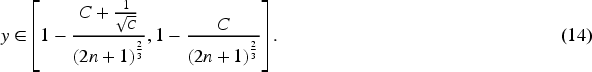
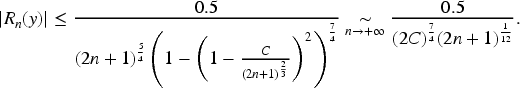
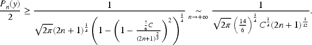
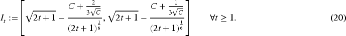
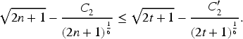
For any fixed constant , for any and any in the interval
the following inequality holds uniformly
In the sequel, we only need the previous result for a single choice of , for instance the smallest one . In particular, we note that an immediate corollary is the bound
which is known to be optimal for (see Thangavelu, 1993, Lemma 1.5.2).
A numerical computation shows that the upper bound is less than . Finally, the condition (19) proves that belongs to and hence .
For the multidimensional case, the following corollary will be required.
Let be a constant as in Proposition 3 and fix satisfying . Moreover, we consider . Define the following intervals
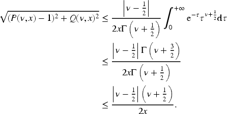
For any and satisfying , the following inequality holds
For simplicity, we use the following notations:
We will show that if is chosen small enough then the inequality implies that the interval is included in the one appearing in (13):
By invoking Proposition 3, such an inclusion will yield the uniform bound for , which in turn implies the expected bound (21) because for .
We first compare the lower bounds of the two intervals and we have to show the inequality
The sequence is increasing, which allows us to apply the bound
and
It suffices to show for that the last upper bound is less or equal to
It is clear that it is sufficient to set .
For the comparison of the upper bounds of the two intervals, we briefly give the similar arguments. We use so that it is sufficient to prove the inequality
that would lead to the sufficient condition .
Cardinality of the Set
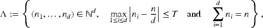
We require a combinatorial lemma in which we will work under the assumptions and for .
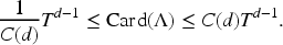
For any integer , there exists a constant , with the property that, for any and any real number satisfying , the cardinality of the set defined below is of order :
The case follows directly from
In what follows, we assume .
Step 1. The upper bound follows from the fact that each belongs to . Thus runs over a set of size and is determined by the choice of the first integers.
We now explain the lower bound of .
Step 2. Let be non-negative integers satisfying for each
The integer satisfies
We have just identified an element of .
Step 3. In order to construct other elements of , consider satisfying
The number of tuples is . For , we will use the following consequence:
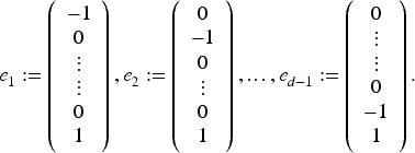
We now introduce the following linearly independent vectors:
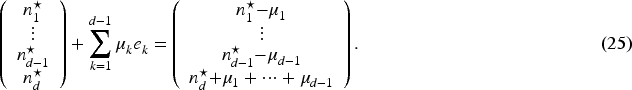
We claim that all the above conditions ensure that the following point belongs to :
It is clear that the sum of the coordinates equals .
We now check
Such inequalities come directly from (22), (23) and (24).
We finally note that (26) and the assumption show that each coordinate of (25) is non-negative.
Proof of Theorem 1
Let as in Proposition 3. In particular, . We fix so that we can apply Corollary 5. We then set
In particular, one has . Lemma 6 then ensures that, for , the set has size of order . Consider the interval defined in (20) for . For any belonging to the subset , the following holds:
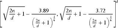
A numerical computation allows us to restrict to the following hypercube:
whose volume is of order . We finally integrate the norm in of the function equalling on this hypercube to get the conclusion:
Appendix: Explicit Inequalities About Airy Functions
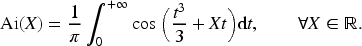
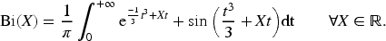
We recall several notations and write explicit inequalities which are consequences of Olver (1997). The Airy function is defined as the improper integral
As , the following asymptotic is known:
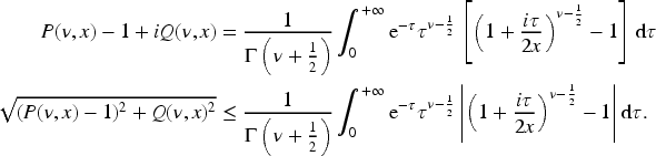
We require the following result that gives a quantitative statement of the oscillating behaviour on .
The following holds true for any :
Moreover the constant is optimal.
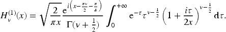
Fix , we shall consider the first Hankel function which may be defined by the following formula (see Watson, 1945, page 168, line (3) or Olver, 1997, page 268, lines (13.01) and (13.07)) for positive :
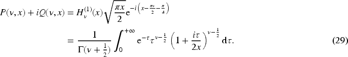
Following Olver (1997, page 269, Ex 13.1), we introduce two real terms4 and as follows:
Since the following inequality will be needed at the end of this section, we first require :
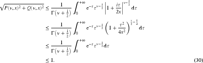
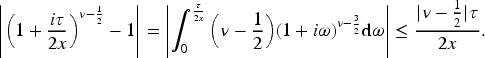
For , we now claim that the following inequality holds true for any :
The proof follows directly from the previous integral representations:
By using , we may invoke the inequality
As a consequence, we continue our computations to prove (31):
For , this inequality reads
We use the following identity, which relates the Airy function to the Hankel function and, consequently, to and (see Olver, 1997, page 392, line (1.05) and then use (29)):
Then (28) is a straightforward consequence of (32) and the last identity.
The sharpness of (28) for is due to the direct appearance of the constant in the classical asymptotics of the Airy function5 :
It is sufficient to make tend to under the condition .
Following Olver (1997, pages 394395), one may define three functions as follows.
The Airy function of the second kind is defined by
Moreover, a formula similar to (33) also holds (see Olver (1997, page 394) by setting or Olver (1997, page 393, line (1.14)) and (29)):
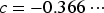
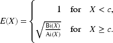
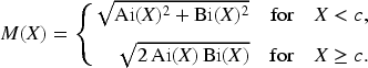
A weight function has a definition involving
the largest negative solution of . We then define
As explained in Olver (1997), the function is non-decreasing and satisfies
A modulus function is finally given by
Note that for any , we may write
From (33) and (35) and then (30), we infer the following
We conclude this section with a remark that will be used below. For any (and thus ), the following identity holds:
Appendix: Proof of Proposition 2
Instead of following the constants in the proof of Skovgaard (1959), we prefer to use the results presented in Olver (1997, page 403, Ex 4.2 & 4.3) since some explicit computations are already provided.
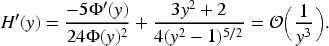
We aim to study the following function for :
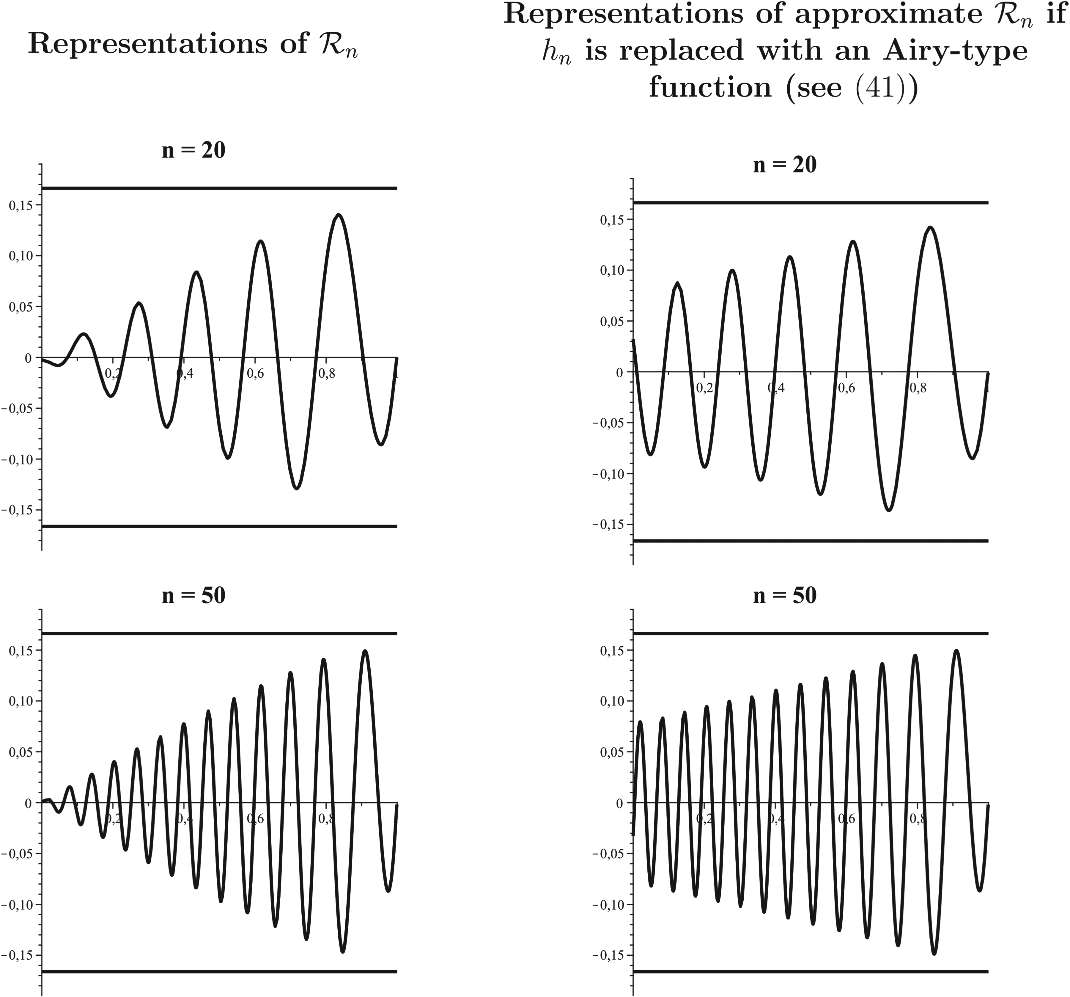
While precise statements are given below, we first note that, as , is approximated by an Airy-type function, in its oscillatory regime, that roughly reads
The figure below shows two graphical representations of for , compared with approximations in which an Airy-type function is used instead of (in fact, the principal term of (41) was employed because it is more precise than (39)).
In particular, we note the following observations:
the two curves are essentially superposed for near , indicating that is well approximated by an Airy-type function near the turning point ,
if the Airy function is replaced with its classical asymptotics at , see (34), one conjectures that a natural expected bound of would be .
However, a residual term in the proof yields a larger upper bound (see (49)), which is sufficient for our purpose (see (18)). Proposition 2 constitutes a special case of the following result.
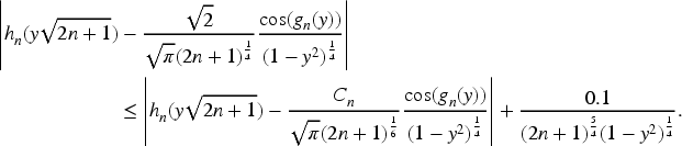
Given any , there exists a constant such that, for all , the following inequality holds uniformly for :
Moreover, for the constant , the value is convenient.
We now outline the main ideas for obtaining an explicit constant in the upper bound of (40).
From (10), the formulas and ensure that it is sufficient to prove (40) for .
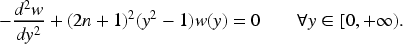
From the differential equation (3) satisfied by , we deduce that the function satisfies the following one:
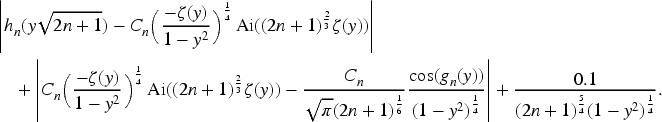
The set of such forms a two-dimensional vector space. We now invoke Olver (1997, page 399, Theorem 3.1) that provides two solutions expressed with the Airy functions and : one solution diverges to as its argument tend to whereas the other tends to . It follows that these two solutions are linearly independent and constitute a basis of the vector space of all solutions. In particular, there is a unique solution, up to a multiplicative constant, that tends to at . Since tends to at , we may use the asymptotic form in Olver (1997, page 399, Theorem 3.1 and page 403, Ex 4.2 and 4.3) and claim that there exists a constant satisfying:
in which the function and the remainder are now given. It should be noted that the factor of the Airy function is essentially constant for (see (47)) and (see (42)):
The function is a continuously differentiable solution of , yielding the classical formulas:
Here is a remark useful for the end of the proof:
which indeed reads
Explicit bounds of the remainder for . Once numerical computations have been performed in the result presented in Olver (1997, Theorem 3.1), the following explicit bounds are reported in Olver (1997, page 403, Ex 4.3) for :
Using (36) and (37) from the previous section, the following inequality holds uniformly in the region for :
Negligible contribution of the remainder as . We use Olver (1997, page 397, line (2.15) and page 403, Ex 4.2) and (38) to obtain
for a suitable explicit function given by
In particular, the derivative of on can be expressed in terms of (see (42)) and satisfies, as :
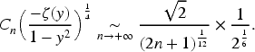
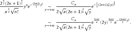
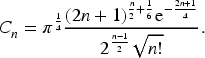
Computation and asymptotics of in (41). We fix and study the asymptotics, as , of the two sides of (41). For the left-hand side of (41), we refer to (2) and recall that is a polynomial with leading term . For the right-hand side of (41), we refer to (46), (27) and use . We then write
The previous comparison leads to the following computation:
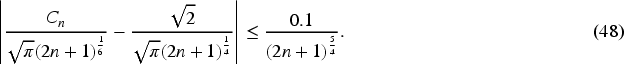
In what follows, we require a two-term asymptotic expansion of the sequence for
and also an approximation of . A numerical computation yields (at this point, we prefer a much larger bound to get a simple final constant in (11)). Consequently, for , the following inequality holds:
Conclusion. We now have all the ingredients to prove (40). We first exploit (48):
By the triangle inequality, the last upper bound can be majorized by
We note that equals with (see (10) and (42)). We may then use the Airy-function approximation (41) and (28) to bound the last term by
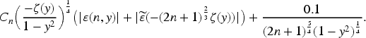
Then (44) and the bound of the remainder in (28) give the following upper bound:
We are now in a position to conclude. We write
and we use (47) and (43) so that we obtain the following upper bound for :
which is less than
The term is the one we referred to as residual before the statement of Proposition 8. Such an upper bound finally proves Proposition 8 because
the last factor is less than for for a suitable near ,
one has and . We deduce that, for small enough, the factor in (50) is less than uniformly for .
Footnotes
Acknowledgements
The author would like to thank Marie Landeiro Dos Reis for motivating the presentation of the results in this article.
Ethical Considerations
Not applicable.
Funding Statements
The author received no financial support for the research, authorship, and/or publication of this article.
Declaration of Conflicting Interests
The author declared no potential conflicts of interest with respect to the research, authorship, and/or publication of this article.
Notes
References
1.
ErdélyiA. (1960). Asymptotic solutions of differential equations with transition points or singularities. Journal of Mathematical Physics, 1(1), 16–26. 10.1063/1.1703631
2.
ImekrazR.RobertD.ThomannL. (2016). On random Hermite series. Transactions of the American Mathematical Society, 368(4), 2763–2792. 10.1090/tran/6607.
3.
JeongE.LeeS.RyuJ. (2024a). Bounds on the Hermite spectral projection operator. Journal of Functional Analysis, 286(1), 110175. 10.1016/j.jfa.2023.110175.
4.
JeongE.LeeS.RyuJ. (2024b). Endpoint eigenfunction bounds for the Hermite operator. Journal of the European Mathematical Society (JEMS), 28(3), 1313–1352.
5.
KochH.TataruD. (2005). eigenfunction bounds for the Hermite operator. Duke Mathematical Journal, 128(2), 369–392. 10.1215/S0012-7094-04-12825-8
6.
KochH.TataruD.ZworskiM. (2007). Semiclassical estimates. Annales Henri Poincaré, 8(5), 885–916. 10.1007/s00023-006-0324-2
7.
MuckenhouptB. (1970). Mean convergence of Hermite and Laguerre series. I. Transactions of the American Mathematical Society, 147(2), 419–431. 10.1090/S0002-9947-1970-99933-9.
8.
OlverF. (1997). Asymptotics and Special Functions. AK Peters/CRC Press.
9.
SkovgaardH. (1959). Asymptotic forms of Hermite polynomials. Technical Report 18, Contract Nonr-220(11), Department of Mathematics, California Institute of Technology, 20.
10.
ThangaveluS. (1993). Lectures on Hermite and Laguerre expansions, Mathematical Notes (Vol. 42). Princeton University Press, Princeton, NJ.
11.
WatsonG. (1945). A treatise on the theory of Bessel functions, second edition. Cambridge University Press.