
Abstract
How do public good spillovers influence agent effort in an interconnected environment? We develop a model for a general class of problems in which agents share the provision of a public good and downstream agents experience spillovers. We characterize endogenous agent effort as the result of their location in the network, their responsibility over the resource, and a regulated facility’s location within the jurisdiction. We examine our findings with an empirical exercise centered on the regulation of 6000 major water pollution sources under the U.S. Clean Water Act. We construct a novel dataset of U.S. state water pollution regional offices and use geographic information on agency jurisdictions, watershed boundaries, and elevation-induced streamflow to characterize the propensity for agents to exert detection effort in their local environment. Our empirical results support our expectations.
Decisionmakers of all stripes face a common challenge: the effects of their decisions rarely stay where they start. The consequences of a given decision often spill over into other domains, affecting other actors, and creating new challenges for policymakers. Changes to a first-grade curriculum ripple through the entire educational pipeline; zoning laws shape not just property values but also how communities develop over time; tax policies might encourage some actors to move across state lines, altering the very problems those policies were designed to address.
No arena is immune to spillovers, but environmental policy is particularly vulnerable. The natural flow of water, air, and wildlife need not align with the administrative boundaries that humans have created, and the consequences of pollution or habitat destruction often extend far beyond the borders of the jurisdiction where the pollution originated. Unlike social or economic policies, where spillovers can sometimes be mitigated through adjustments, environmental spillovers are dictated by physical realities that are much harder to control. This makes environmental policy uniquely challenging, as policymakers must navigate a complex web of interconnected consequences that extend beyond their direct influence.
Institutions charged with managing environmental pollution generally do so by subdividing environmental resources into administrative jurisdictions. These jurisdictions are then charged with overseeing both the resources and any potential spillovers (Gray and Shadbegian, 2004). Upstream governments and private firms can take actions that reduce environmental pollution loads for downstream entities. However, governments with jurisdiction over pollution sources have strong incentive to promote spillover to downwind and downstream jurisdictions when possible (Monogan et al., 2017). Incentives for spillover are more challenging still, when administrative jurisdictions further fragment environmental resources which introduces perverse incentives for regulators and facilities alike (Lipscomb and Mobarak, 2016).
The degree of this fragmentation is critical to understanding how and when spillovers materialize. Fragmented jurisdictions create a complex network of interactions, where each jurisdiction has its own priorities and constraints. When administrative boundaries dissect natural systems, such as watersheds, this misalignment can undermine collective efforts to manage environmental quality. Regulators may focus their efforts narrowly within their jurisdiction, neglecting the broader implications of upstream or downstream pollution. At the same time, firms might exploit jurisdictional divides to reduce regulatory scrutiny or compliance costs.
In this article, we examine how the fragmentation of environmental resources by administrative boundaries affects the incentives of regulatory agents to enforce environmental regulations. Using a formal model, we explore how jurisdictional design and fragmentation influence regulatory effort and facility compliance, focusing on the special case where “gravity goes one way”—that is, where the flow of spillovers follows a partial order. Though indeed special, the case includes important examples such as our motivating case, water pollution (where water flows only downstream), but also policies where consequences of decisions occur latter in time (where time flows only forward), or where decisions are made at different levels of government (where power flows only downward). By highlighting the interplay between fragmented institutions and spillover effects in this structured setting, our analysis contributes to a deeper understanding of the challenges posed by environmental governance in fragmented policy spaces.
Our approach draws from, and contributes to, a diverse set of established theoretical frameworks, particularly in the domain of network games and spillover effects. 1 The foundational work of Bergstrom et al. (1986) inspired a rich tradition in studying effort-exertion games, particularly in contexts where public goods and spillovers are critical. This line of research was significantly advanced by Ballester et al. (2006), who demonstrated that effort-exertion games with finite populations can be decomposed into two key components: a network-game component with local payoff complementarity effects and a global component with payoff substitution effects. These insights highlighted the dual nature of agents’ incentives in networked environments. Bloch and Zenginobuz (2007) extended these ideas by modeling spillover effects that could be either symmetric or asymmetric. Their findings underscored the unique challenges posed by asymmetric spillovers, particularly in achieving equilibrium uniqueness and determining the sign of substitution effects. Similarly, Bramoullé and Kranton (2007) examined the interplay between substitution effects and specialization outcomes, identifying conditions under which some agents exert effort while others strategically free ride.
Closer to our focus, Ogawa and Wildasin (2009) developed a model that captures interactions between agents and firms, though their emphasis was on productivity and jurisdictional transfers rather than regulatory detection. Other notable contributions include Bramoullé et al. (2014), who showed that the lowest eigenvalue of a network serves as a sufficient statistic for understanding how other agents’ behavior influences a given agent’s choices. This result points to the importance of well-partitioned networks in achieving optimal regulatory outcomes. Allouch (2015) further advanced this tradition by providing a general existence result for network games of good provision, focusing on resource distribution among consumers rather than regulatory effort. Building on these foundations, Elliott and Golub (2019) explored how the spectral properties of networks influence welfare outcomes, integrating insights from both Bramoullé and Allouch. Finally, Galeotti et al. (2020) studied the effects of policy interventions on welfare in large networks, demonstrating that simple interventions often yield the best outcomes.
While many of these theoretical advances are motivated by environmental concerns, they remain abstract and detached from the specific challenges of regulatory enforcement. Few provide actionable insights without imposing significant additional structure, and those that do often leave empirical validation as an open task. Moreover, none of the existing literature models the strategic interaction between regulators and facilities in a fragmented resource context. We address these gaps by developing a formal framework to study water regulation in a fragmented policy space. Our model combines insights from network games with a well-specified structure of spillovers. Facilities are embedded within a network, where ties—representing spillover intensity—are determined by physical properties such as proximity and flow size. Facilities choose compliance levels with local regulations, while regulatory agents decide how much effort to allocate toward detecting noncompliance within their jurisdiction.
Our theoretical contribution is twofold. First, and more generally, we provide conditions under which the regulatory game admits a pure-strategy Nash equilibrium. These conditions are largely independent of the network’s specific structure, allowing us to study and compare networks with varying degrees of spectral tidiness. Second, and more specifically, two parametric vignettes illustrate simple mechanisms for how regulatory effort is influenced by jurisdictional design. Our results show that regulators exert less effort at facilities near the “bottom” of their jurisdiction, whereas upstream regulators allocate more effort when their authority over their jurisdiction is greater.
We evaluate insights from our model in the context of government agents tasked with providing public goods in the form of watershed protection. The imposition of administrative boundaries on a policy domain imposes a network structure that shapes agents’ incentives to exert effort in delivering the public good. Specifically, we consider the artificially-created administrative boundaries that shape the quality of an agent’s jurisdiction by dissecting watersheds. These dissections place limits on agents’ responsibility for managing resources under their discretion and impose downstream relationships. In such settings, under certain conditions, spillover may incentivize agents to use their discretion to select effort levels that undermine the provision of the good. In other words, governance gaps between political and environmental boundaries induce coordination challenges across agents (Ekstrom and Young, 2009), but the degree to which this matters for policy delivery depends on the nature of the fragmentation and spillovers that result.
We examine our expectations using a newly-constructed dataset of U.S. state regional offices charged with water pollution control responsibilities. These regional administrative offices are created by state environmental agencies and are used to regulate activities under the U.S. Clean Water Act, such as permitting and compliance assurance. Using GIS software, we generate a novel dataset that spatially delineates each regional office’s administrative jurisdiction and its overlap with watershed boundaries. We further use elevation and stream flow data to demarcate whether the portion of a watershed within a given administrative jurisdiction is upstream or downstream from adjacent regional offices. We then use linear random-effects generalized least squares (GLS) regression analysis to investigate the degree to which higher levels of environmental resource (i.e. watersheds) boundary fragmentation by administrative boundaries results in less regulatory effort from regional agents. The subjects of the analysis are the roughly 6000 major water pollution facilities for which we have detailed historical data on compliance and regulatory activity under the Clean Water Act.
In Section 1, we introduce the model and our analysis of the problem. In Section 2, we consider the specific case of spillovers in water pollution enforcement in the US. In Section 3, we introduce our empirical strategy and we present our results. We then conclude.
A theory of regulation with ordered spillover
In this section, we develop a formal model of environmental regulation with ordered spillovers. In our model, we consider two questions in turn. First, we examine how a single regulator expends effort across multiple facilities within an administrative jurisdiction. Second, we investigate how the extent of watershed dissection by administrative jurisdictions shapes two neighboring agents’ regulatory efforts.
We draw upon a broad literature on agent motivations in regulatory enforcement to guide our setup. Agents pursue enforcement decisions to maximize net political support by securing lower pollution for the least cost (Peltzman, 1976; Stigler, 1971). Enforcement decisions reflect a combination of detection effort and punishment selection (Becker, 1968; Ehrlich, 1973). While punishment selection may range from maximal to either flexible or pragmatic enforcement (Gunningham, 2011; Hunter and Waterman, 1996; Scholz, 1991), detecting noncompliance is foundational to any of these tactics. With respect to detection effort, regulators typically pursue a dual-group auditing framework. Regulators divide facilities into at least two detection target groups based upon past compliance records. One groups consists of higher priority facilities with more troublesome compliance records and the other group contains lower priority facilities with more cooperative histories (Friesen, 2003; Harrington, 1988). Regulators adjust their detection efforts across these facility groups to gain returns in the form of specific and general deterrence against noncompliance (Gray and Shimshack, 2011). With these lessons in mind, we now introduce our model.
We take as primitive the domain, which is a pair
The strategic-form game played in the domain includes two classes of players.
The first class of players is a finite, but not empty, set of regulators, The second class of players is a finite, but not empty, set of facilities,
Nothing precludes
The two classes have distinct available strategies.
Each regulator decides how hard to inspect compliance at each of her regulatory candidate facilities. Formally, this is an effort vector Each facility decides how much to comply with regulations. Formally, Facility
A strategy profile is a pair tuple

The regulators’ and facilities’ respective decisions influence the relevant political-geographic outcomes via two mechanisms. Politically, they determine each facility’s probability of detection. Formally, we introduce the probability of detection,
The probability of detection Effort Monotonicity: Compliance Monotonicity:
In words, the continuity assumption asserts that small changes in effort or compliance map to small changes in the probability of detection; Effort Monotonicity asserts that more regulatory effort yields higher chances of detection; and Compliance Monotonicity asserts that more compliance yields lower chances of detection.
Geologically, noncompliance harms water quality. Define
(Water Quality)
For all locations Compliance Monotonicity: we have Convexity in Local Effort: for all Fluidity in the Stream: the map
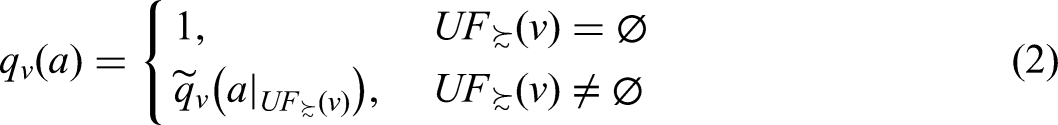


In words, the functional form assumption asserts that the water quality at a given location depends only on behavior upstream; the continuity assumption asserts that small changes in regulatory effort and compliance yield small changes in quality; Convexity in Local Effort asserts that the quality at location
The two classes of player have different kinds of preferences over these consequences. For each regulator
For all regulators Quality Monotonicity: Effort Monotonicity:

In words, the functional form assumption asserts that a regulator’s utility depends only on the quality across locations in her jurisdiction and on how much effort she has exerted; the continuity assumption asserts that small changes in quality and effort yield small changes in regulator utility; Quality Monotonicity asserts that a regulator does better when her locations feature higher quality; and Effort Monotonicity asserts that effort is costly.
As for the facilities, we introduce
For all facilities Compliance Monotonicity: Fear of Detection:

In words, the functional form assumption asserts that a facilty’s utility depends only on how much it complies and on the probability it is detected if non-compliant; the continuity assumption asserts that small changes in compliance or probability of detection yield small changes in utility; Compliance Monotonicity asserts that compliance is costly; and Fear of Detection asserts that facilities do worse when they expect to be detected.
This is a strategic-form game, and we are interested in its pure-strategy Nash equilibria. We can say the following.
Any regulatory game in the domain has at least one pure-strategy Nash equilibrium.
The result is a straightforward application of the Debreu-Glicksberg-Fan theorem; we provide a proof in the Supplemental Appendix for completeness, but the required continuity and quasiconcavity assumptions are all satisfied by our setup.
Vignettes
To provide some simple actionable mechanisms, we introduce two vignettes. In both, we have
Regulators work less downstream
We first consider how a single regulator expends effort across multiple facilities. Suppose—for now—that there is a single regulator,
The regulator inspects the two facilities by choosing a pair of effort levels
For both facilities

Sample
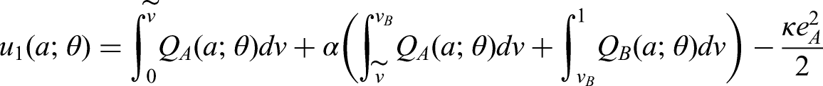
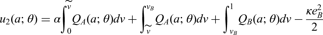
Finally, preferences. The regulator is concerned with water quality across


For both facilities
The logic here is straightforward: if a facility were perfectly compliant, then the regulator would spend no effort there, which in turn would incentivize the facility to comply less, breaking equilibration. This raises questions about how the regulator behaves at the two facilities. Next, we see that the regulator is constantly vigilant save for the limiting case where the downstream facility is situated exactly at the bottom of the watershed.
(Vigilance Save for the Bottom)
In other words, the regulator is always willing to work so long as there are some downstream benefits of doing so. In the limit, effort disappears when
(When the Cat’s Away)
For both
Thus, the conditions that lead to zero effort also lead to zero compliance. However, the converse need not be true: a given facility might comply minimally while the regulator inspects in the name of mitigating the deleterious environmental consequences of extreme noncompliance.
With these three lemmas in place, we can now state the main result of this section: as the downstream facility is moved closer to the limit of the regulator’s jurisdiction, the regulator eventually expends negligible effort there, and the facility eventually exhibits negligible compliance.
(Convergence to the Bottom)
Let

Proposition 9 informs our first hypothesis (stated in the next section), and its logic is straightforward. Given the myriad possibilities regarding how polluted water impacts the environment downstream, we cannot make any promises that regulators expend less effort as the downstream facility moves further downstream; after all, it would well be that
Upstream regulators work harder when they control more
We now study the relationship between watershed autonomy and regulatory effort.
We continue to study two facilities
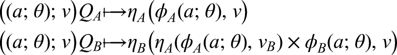
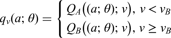
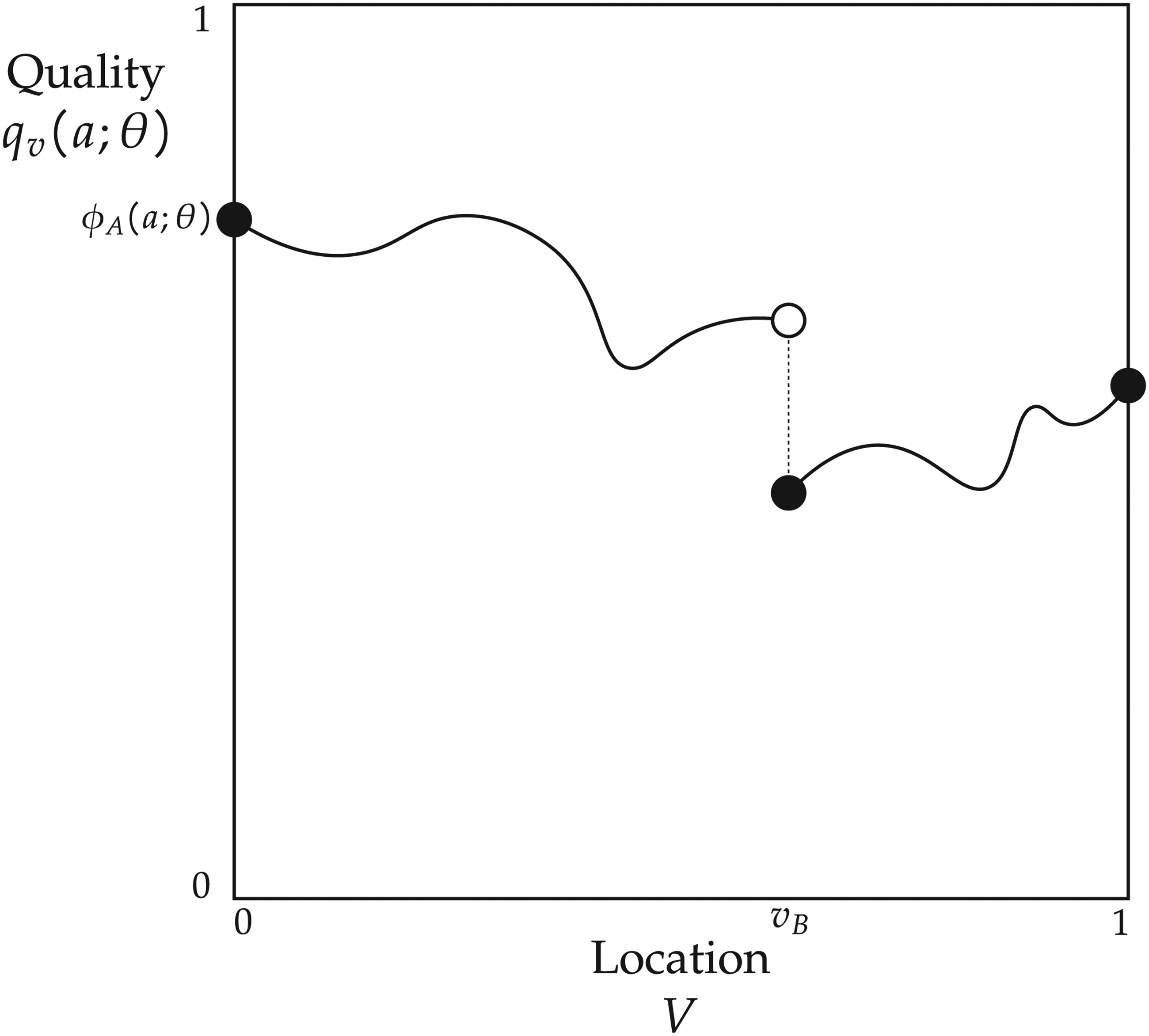
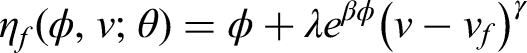
We now provide a straightforward parameterization of the model’s environmental aspects. We keep the instantaneous effects
As for preferences, we keep the von Neumann-Morgenstern expected utilities for the facilities. Regulator 1’s preferences take the form
This game still has at least one pure-strategy Nash equilibrium, and Lemmas 6 to 8 continue to obtain. 6 We therefore are in position to state our main equilibrium result.
(Upstream Agents Work Harder When Responsible for More)
In any Nash equilibrium of the game described in this section,
Proposition 10 informs our second hypothesis, and its logic is also straightforward. The location
We now turn to evaluating our two hypotheses summarized below:
In the next sections, we consider the case of water pollution in the US and then discuss our empirical research design to test these hypotheses.
Water pollution control and spillover in the United States
The management of U.S. water pollution provides an ideal empirical setting to study spillover problems that arise when environmental resource and governance boundaries do not match. The primary federal statute that addresses discharges of water pollutants into U.S. waterways is the U.S. Clean Water Act (CWA). 7 Similar to other major U.S. federal pollution control statutes, the CWA is largely implemented under a model of cooperative federalism in which the federal government (i.e. the U.S. Environmental Protection Agency, or EPA) has the principal authority to set standards, but then hands over implementation responsibilities to willing state governments. More specifically, for point sources of pollution (e.g. factories, power plants, and municipal wastewater plants) that release effluent directly into U.S. waters, the EPA sets technology-based limitations. As a backstop to these limits, the CWA obligates states to set water quality standards, which may result in further effluent limitations so as to assure that a specific water resource is achieving its designated uses (e.g. drinking, fishing, swimming, etc.).
Of most relevance for our study is that the EPA has largely delegated implementation of the CWA to state agencies. State environmental offices carry out the largest share of permitting, compliance monitoring, and enforcement activities for the hundreds of thousands of individual sources of water pollution in the United States. By one estimate, over 90% of the environmental enforcement in the United States is generated by state pollution control agencies rather than the EPA (ECOS, 2001). Given inevitable variation in how states decide to pursue these activities, it is no surprise that states feature prominently in scholarly treatments of U.S. environmental regulation (e.g. Hunter and Waterman, 1996; Konisky, 2007; Lowry, 1992; Potoski, 1999; Ringquist, 1993; Wood, 1991, 1992). In fact, much of what we have learned over the past three decades about the effects of politics, economics, and administrative features on U.S. environmental implementation rests on the foundation that states are the most relevant level of government for analysis.
Despite this considerable attention, scholars have black-boxed important institutional features of state environmental agencies, including their geographic organization. Most states do not implement policy via the state capital, but rather they have decentralized it to regional offices distributed throughout the state. The logic of this devolution is driven, at least in part, by a desire to manage demanding workloads efficiently and to be more responsiveness to local needs (Woods and Potoski, 2010). Nevertheless, extant research in environmental regulation has virtually neglected state regional offices as unique policy delivery institutions in their own right (Reenock et al. (2022) is an exception). In so doing, scholars have not examined the extent to which this geographical carving up of state policy implementation induces coordination problems. Dissecting administrative responsibility of a resource introduces two intimately-linked geographic challenges for regulation. It creates multiple parties responsible for the resource’s management, and in doing so, it also situates at least one of these parties as being downstream from the other.
To illustrate this situation, consider Figure 2, which overlays U.S. watershed boundaries with state regional water pollution control offices. It is rare for state regional offices to follow watershed boundaries. Instead, watersheds, and, therefore, their associated rivers, typically span two or more regional offices. In most cases, states have demarcated their regional offices by groupings of coterminous counties in a manner that does not account for watershed boundaries. In fact, for all watersheds in the figure, the average percentage of a watershed fully contained within a state regional office is 75% with a standard deviation of 27%. It merits mentioning that, state boundaries, of course, also span across watershed boundaries. However, the types of problems that arise from interstate management of water resources have received more attention in the literature (Bowman and Woods, 2007; Heikkila and Schlager, 2012; Schlager and Heikkila, 2009; Woods and Bowman, 2018) than the types of intrastate issues emphasized here.
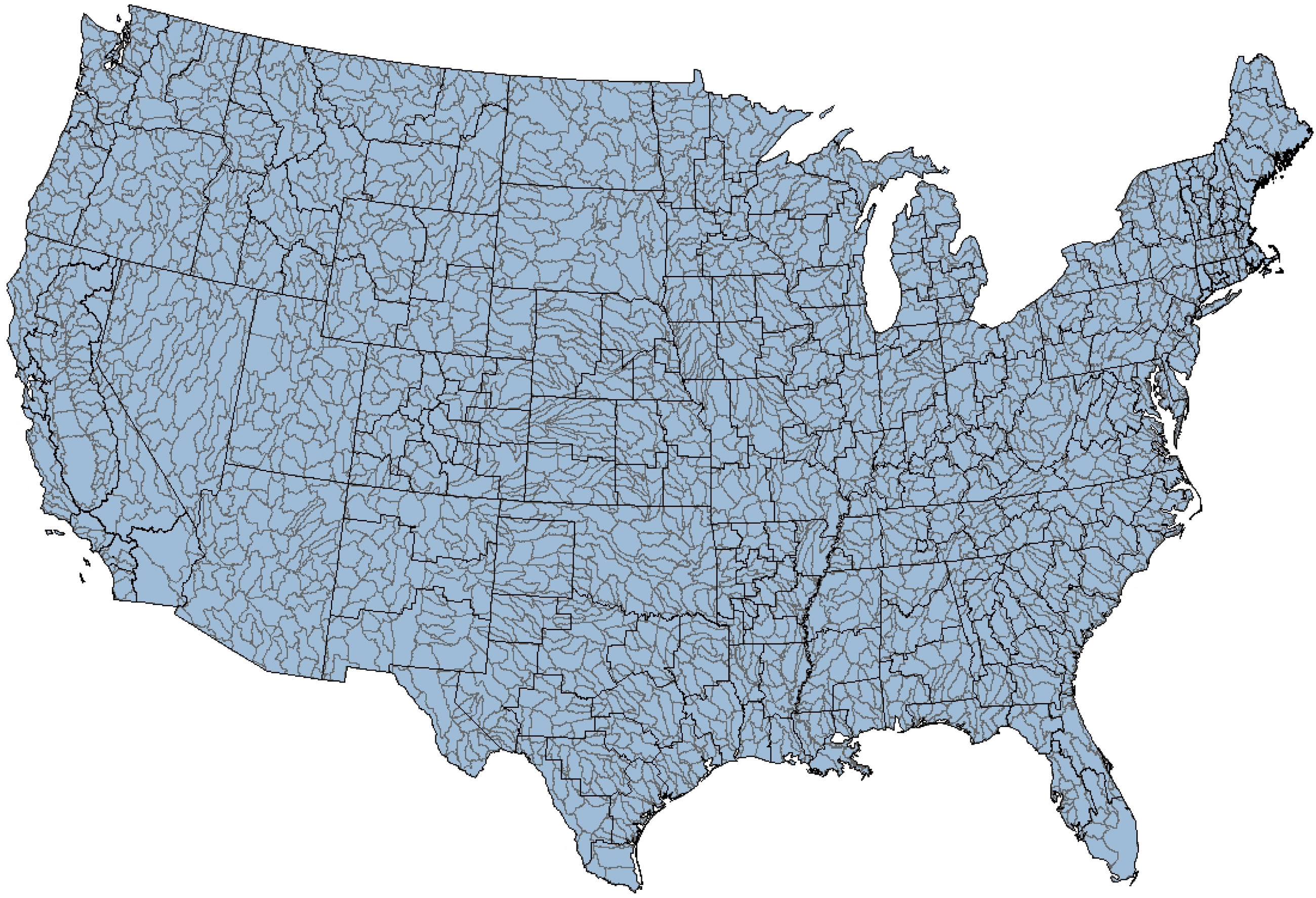
State regional offices and watershed boundaries.
To further illustrate, Figure 3 displays the regional office and watershed boundaries for California, which stands alone in its effort to consider watershed boundaries when drawing its regional offices boundaries. The nine regional offices in California have boundaries that nearly fully encompass their covered watersheds. In California, the average percentage of a watershed contained within a state regional office is 99% with a standard deviation of 3.0%. Other state agencies, by contrast, routinely dissect watersheds. Georgia and Wisconsin, in the other two panels, are not as mindful of watershed boundaries. In Wisconsin, the average watershed amount that is fully contained within a state regional office is only 72%, with a standard deviation of 26%. Watershed dissection is even more pronounced in Georgia where the average amount of a watershed that is fully contained within a state regional office is only 62%, with a standard deviation of 29%.
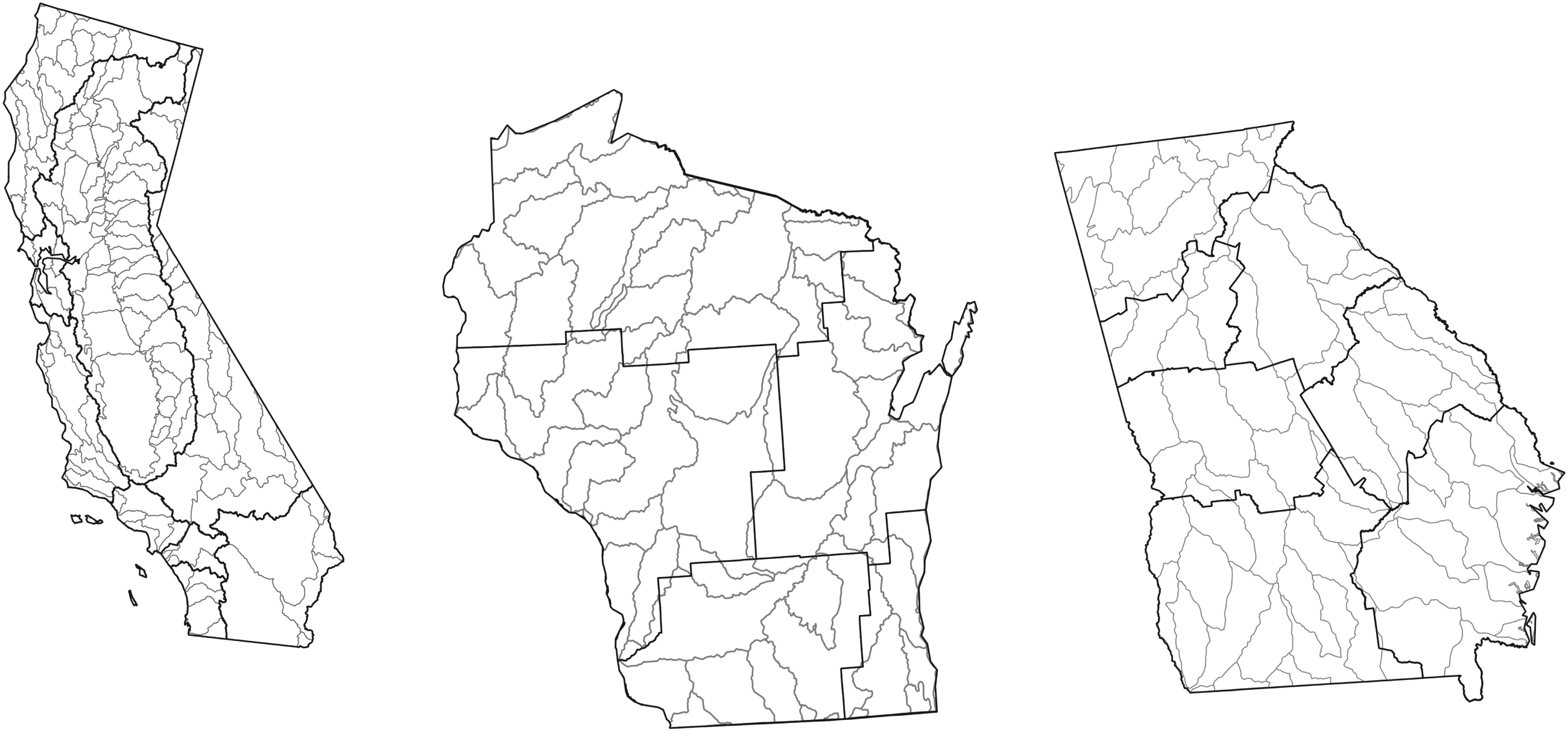
California, Wisconsin, and Georgia state environmental agency water division regional offices.
But dissecting a watershed also induces another challenge: directionality. Discharges of pollutants into waterways may not only diminish proximate water quality, it may also adversely affect water quality in downstream locations. A closer look at the case of Georgia illustrates this point. In Figure 4, we have added major rivers and the location of point sources water pollution regulated under the CWA to the map. Consider the area highlighted in red. This watershed is split between Georgia’s Mountain District office (to the north) and its West Central District Office (to the south). The major river in this watershed is the Flint River, and it flows from north to south. In this case, agents in the upstream Mountain District office may have incentive to exert less enforcement effort on facilities located nearest the downstream regional office border.
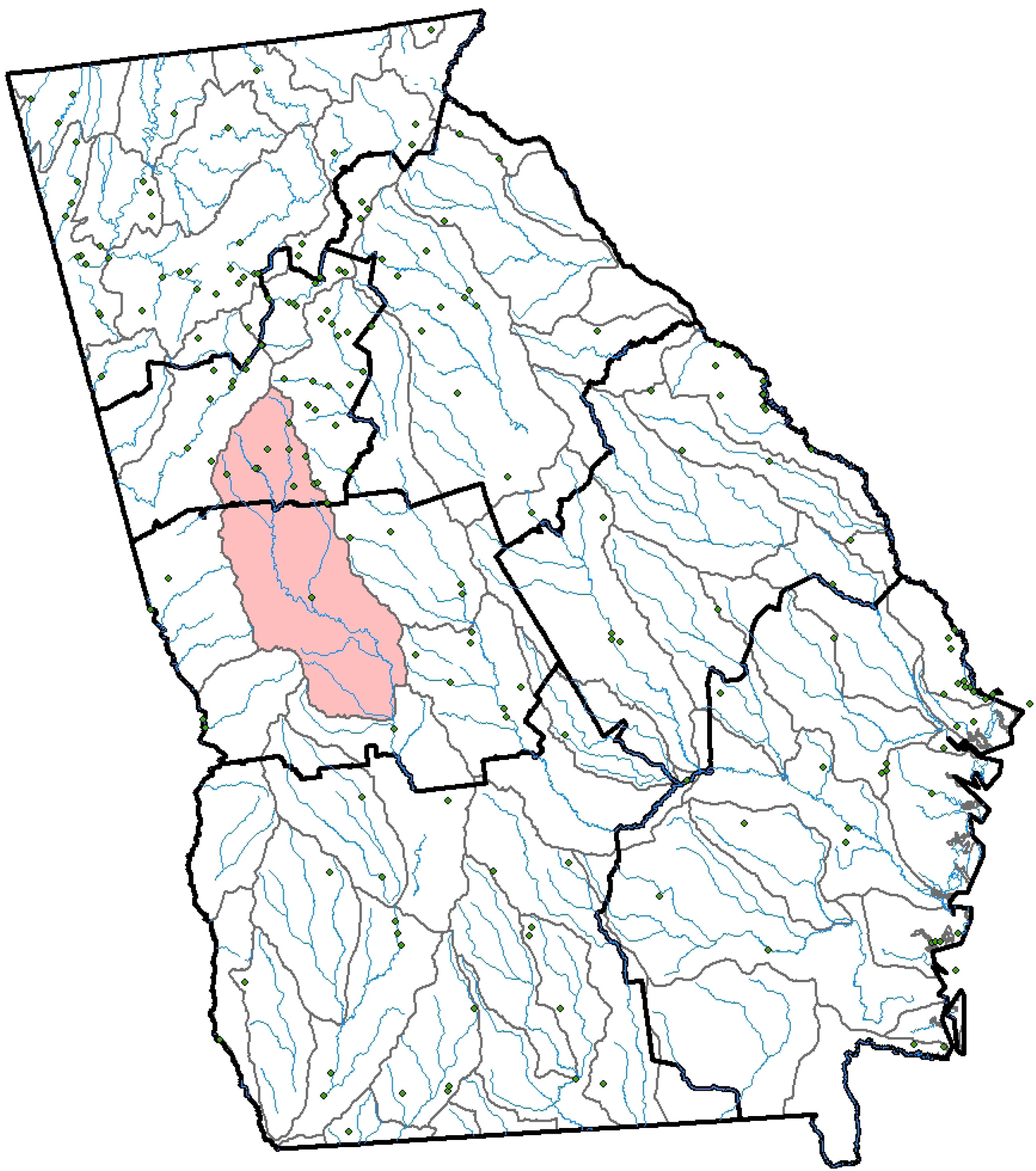
Georgia Environmental Protection Division’s seven administrative water regions and overlaid watersheds. Circles are major water facilities. Flint River watershed is shaded region.
How might agents responsible for regulating facilities under the CWA respond to the two geographic challenges induced by dissecting an environmental resource? Our model provides two expectations, which, in the next section, we discuss our research design that we employ to test these hypotheses.
To examine our propositions, we created an original dataset that combines administrative data on regulatory compliance and enforcement, watershed boundaries, streamline and elevation data, 8 and state administrative agency boundaries. We discuss each in turn.
Regulatory Compliance and Enforcement. The EPA maintains extensive historical records on facility-level compliance with most major pollution control laws, as well as regulatory actions taken by federal and state officials to enforce these laws. In the case of the CWA, we use data from the EPA’s Integrated Compliance Information System-National Pollution Discharge Elimination System (ICIS-NPDES) dataset. 9 The ICIS-NPDES archives facility-level violations of and compliance with the CWA (i.e. not all violations result in an determination of noncompliance as defined by EPA guidance), and individual enforcement actions taken by the EPA and state government agencies (e.g. compliance monitoring inspections and punitive measures). The data include a diverse set of facilities that are required to have NPDES permits under the CWA (under the law, any point source discharging pollutants directly into a U.S. waterway is required to have a NPDES permit), but, since reporting is only required for “major” NPDES sources, we limit the scope of our study to these facilities. 10 During the time period of this study, there were about 6700 facilities with major NPDES permits, although we analyze a slightly smaller number (about 6400) because some major facilities are located in states that the EPA had not yet delegated authority to implement the CWA (Idaho, Massachusetts, New Hampshire, and New Mexico), and because of some missing data. 11
Due to data constraints on state regional office information, our timeframe is limited. As such, we create several measures using the ICIS-NPDES data for the years 2001–2014. First, the dependent variables we analyze come from the regulatory output data included in ICIS-NPDES. Specifically, we create annual counts of state-led inspections directed toward each major NPDES permitted facility, distinguishing between sampling inspections (i.e., inspections in which government officials conduct independent sampling of a facility’s discharges) and non-sampling inspections (i.e. inspections that do not include independent sampling and reflect a review of facility records). 12 We present the results for sampling inspections in text as they reflect a higher level of agents’ detection effort; results for non-sampling inspections, which reflect a lower level of agent effort are reported in the Supplemental Appendix. These measures are frequently used in the social science literature to capture the regulatory effort of government agencies to enforce the CWA (Gray and Shadbegian, 2004; Helland, 1998; Konisky and Reenock, 2013; Konisky, 2007; Scholz and Wang, 2006).
The ICIS-NPDES data also include quarterly determinations of a facility’s noncompliance status with the CWA. In particular, the EPA tracks two types of noncompliance: reportable noncompliance and significant noncompliance. Significant noncompliance is the more serious designation, and can be triggered by effluent violations (i.e. discharges that exceed permitted limits), failure to submit a discharge monitoring report, violation of a previously-set compliance schedule, or a violation identified during a government inspection. Reportable noncompliance are instances of noncompliance that do not rise to the level of significant noncompliance. In the analysis that follows, we create dichotomous, annual measures of each noncompliance type for each major NPDES facility.
In sum, we create a facility-year level dataset of compliance and regulatory actions for about 6400 major NPDES sources. These facility-level data are then combined with the geographic data we describe next. 13
Regional Office Boundaries, Watershed Boundaries, and Downstream Border Distance. To examine our hypotheses regarding the dissection of watershed boundaries and policy coordination, we collected four additional sets of geographic data. First, we obtained information on the geographic organization of each state agency, which we compiled in earlier research from state agency websites or other documents we collected from contacting state officials. This information was confirmed in telephone interviews with officials in each state agency. These are the data we previously presented in Figure 2. We then used GIS software to delineate the jurisdiction of each office. 14
Second, we collected information on watershed boundaries from the U.S. Geological Survey’s (USGS) Watershed Boundary Dataset. The USGS classifies all watersheds in the United States using a numerical coding system that assigns each a unique hydrologic unit code (HUC). In our analysis, we use cataloging units, which are geographic areas that represent part or all of a surface drainage basin, a combination of drainage basins, or a distinct hydrologic feature. Each watershed represents a natural topographical basin within which surface water drainage exits via a single outlet. There are 2264 such cataloging units in the United States.
Our measure of watershed intersection accounts for the degree of control that an agent has over a watershed. This formulation is more consistent with our theoretical propositions than treating dissection as a dichotomous condition, since we posit that the degree of effort exerted by an agent depends on how much a watershed is split across administrative regions. We measure watershed dissection as the watershed’s proportion that is contained within the boundaries of a given regional office, which we delineate using geographic area (measured in square miles). Of the 2111 watersheds in the continental United States, about 15% are contained wholly within a single state regional office.
15
In these cases, our dissection metric is equal to one (i.e. agents control the full area of the facility’s watershed). Many of these are watersheds located within states that do not makes use of regions—the entire state is a single administrative region. There is considerable variation in the proportion of a watershed area managed by regional officers. For the facilities in our data, the overall mean and standard deviation of watershed dissections are 0.74 and 0.28, respectively. This measure is the key variable we use to test our first hypothesis. The remaining 85% are intersected in some way by regional office boundaries. Of the
To determine which regional office is upstream or downstream for cases of shared environmental resources, we collected and processed two additional sets of data. First, we used the USGS Flowline Dataset to delineate the major stream in each watershed. We then overlayed elevation measures from the USGS National Elevation Dataset to determine the elevations along each major stream. Using this information we then calculated the maximum elevation height for the stream within each regional office-watershed segment. We then created a variable coded one if the elevation value for a given regional office-watershed segment exceeded that of each of the other regional offices sharing jurisdiction over the watershed. Alternatively, if the elevation value for or a given regional office-watershed segment is less than that for the other regional offices, we coded the variable as zero. 16 With this dichotomous coding, therefore, a value of one represents “upstream,” and a value of zero represents “downstream.”
We also create a variable “downstream border distance,” to asses whether agents distinguish between facilities located far from a downstream border and whose effluent is more likely to be retained in their jurisdiction and facilities located near a border and whose effluent is more likely to spillover into a neighboring region. This measure is calculated as the distance, as the crow flies, between the facility and the closest administrative border that is downstream from it. The average distance to the nearest downstream border is 9.78 miles, with a standard deviation of 8.97 miles. Nearly 25% of facilities in our data are less than a 0.25 miles from a downstream border.
For both of the prior variables, streamflow direction and downstream border distance, we only calculate these measures for watersheds that are shared with another administrative region. The 15% of watersheds that are fully contained within a region are dropped from our analysis. This is because a fully-contained watershed that is either is up or downstream from another watershed within the same region elicits no effort dilemma for an agent—the watershed’s effluent is fully contained in the region regardless of streamflow direction. Only watersheds shared with other administrative regions elicit the spillover dilemma we are investigating. Given that our results may be sensitive to what constitutes a “fully contained” watershed, we consider three thresholds of this delineation. For our analyses, we report three estimates for each threshold of what constitutes a fully-contained watershed. The highest threshold, 1.0, requires 100% of the watershed to be fully contained within a state administrative region. However, we also include analyses in which this threshold is relaxed to .95 and .90 of the total watershed.
Estimation strategy
To examine the relationship between watershed control, streamflow direction and state regulatory enforcement actions, we estimate GLS random-intercept linear regression models,
17
with robust standard errors clustered on facilities, of the following basic form:
To examine the relationship between watershed control, downstream border distance and state regulatory enforcement actions, we estimate the same GLS models but with a new interaction term, of the following basic form:

We address three possible sources of endogeneity: omitted variable bias, sample selection, and reverse causality. To minimize the threat of endogeneity due to omitted variable bias and sample selection, we include a large suite of control variables to adjust for any possible factors that may incentivize firm location choice and firm compliance decisions. To account for confounding factors related to regulatory enforcement outcomes, our models include numerous facility, regional, and state level control variables. At the facility level, we include facility age (based on the date the facility received its first NPDES permit), a series of dichotomous variables to distinguish publicly owned treatment works (POTWs), and industrial dischargers that are either in the electric power sector or in the manufacturing sector. In addition, we created “neighborhood” level demographic measures for each facility. Specifically, we used an areal apportionment method common to the environmental justice literature (Konisky and Schario, 2010; Mohai and Saha, 2006), in which, with GIS software, we estimate the percentage of the population within a one-mile radius circle of each facility that is African-American, Hispanic, below the federal poverty level, and college educated. Also at the facility level, we control for whether the facility was in either reportable or significant noncompliance status during the year, since regulatory enforcement activity is likely to be greater if a facility is determined to be in violation of the CWA.
At the region office level, we include two variables to account for state regulators’ overall task environment: the total number of major NPDES facilities in the region and the total number of all (major and minor) NDPDES facilities in the region. 18 We include similar measures at the level of regional office-watershed section; this is the unit of geography representing the overlap of the regional office and watershed boundaries. These measures control for the more local task environment facing regulatory agents.
Last, we control for a set of state and federal level factors that are commonly included in models of state regulatory enforcement. To account for state economic and political factors that may influence overall enforcement efforts, we use: state unemployment rate, gross state product, the partisan identification of the governor (coded one for a Democrat, and zero otherwise), and the percentage of the lower chamber of the state legislature that are Democrats. In addition, we limit our analysis to states delegated authority to implement the CWA by the EPA. At the federal level, we include a dummy variable coded one for the George W. Bush Administration and zero for the Barack Obama Administration, a variable to capture differences in party control of the U.S. Congress (coded one for unified Republican control (2003–2006), negative one for unified Democratic control (2008–2010), and zero otherwise), and dummy variables for EPA regional offices.
On threats of endogeneity due to reverse causation, we believe that it is a reasonable assumption that enforcement decisions have no impact on the proportion of the watershed under administrative control nor whether that watershed is upstream/downstream. This is due to the fact that administrative boundaries, whether intra-state or inter-state, are temporally stable in our data. These state administrative regions were put in place in the 1970s and have essentially remained constant as the main enforcement delivery mechanism to the present. While regional offices have shifted in a few states over time, these changes are rare and minimal in their impact on a state’s overall regional office makeup.
Results
We report complete model estimates for both empirical exercises in the Supplemental Appendix. Supplemental Table A.1 reports the estimated relationship between regulatory officer agency and a shared watershed’s relative upstream location while Supplemental Table A.2 reports the estimated relationship between regulatory officer agency and a facility’s relative upstream distance from the closest downstream border. Both empirical investigations offer support for our expectations. 19
For each of the models below, we report three sets of estimates with different thresholds of what constitutes a fully-contained watershed. The highest threshold, 1.0, requires 100% of the watershed to be fully contained within a state administrative region. The remaining thresholds reduce this requirement by 5% each at .95 and .90 proportion of the total, respectively.
Table 1 displays the key coefficients from the full inspections models that provide a test of whether regulatory officers’ effort is jointly motivated by enhanced control over their watershed and the relative location of their watershed in the network. The estimates suggest that the proportion of the watershed under regional officers’ control motivates their behavior but is conditioned by the policy context of their responsibilities. The association between officer agency (area) and detection effort is null (or negative) for downstream agents but is positive for upstream agents. To illustrate this conditional relationship, we consider the marginal effect of the area controlled over policy context in a series of marginal effect plots. Figure 5 displays the marginal effect of the proportion of area controlled plotted over streamflow direction with Panels A, B, and C showing the effects for different thresholds of what constitutes a fully-contained watershed at 1.0, .95, and .90 proportion of the total, respectively.
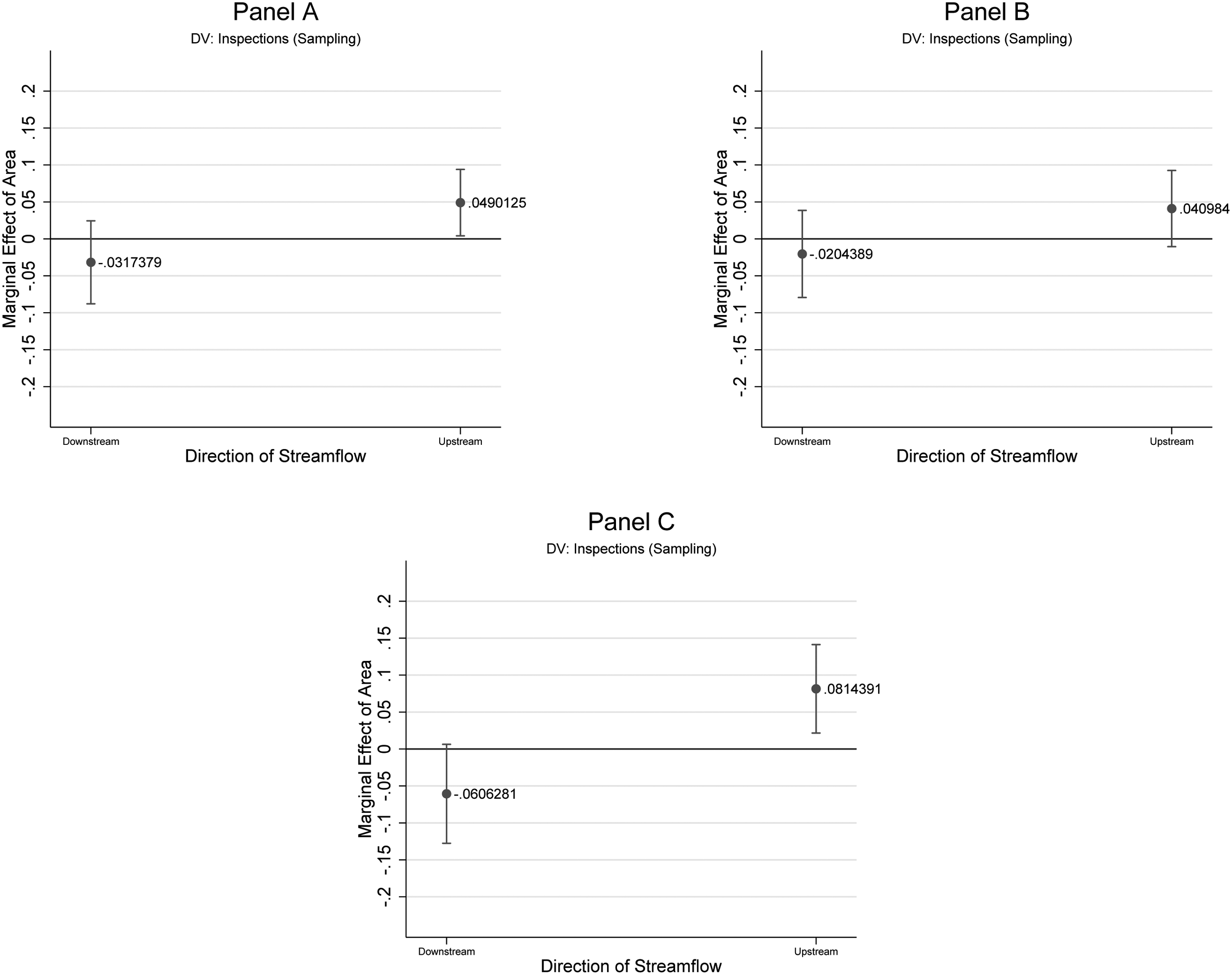
The marginal effect of the proportion of the watershed controlled over being downstream versus upstream by different enforcement outputs.
Parameter estimates estimating regulatory actions.
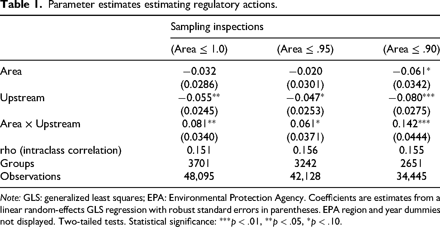
Note: GLS: generalized least squares; EPA: Environmental Protection Agency. Coefficients are estimates from a linear random-effects GLS regression with robust standard errors in parentheses. EPA region and year dummies not displayed. Two-tailed tests. Statistical significance:
On the left-hand side of each plot, we see that controlling one’s watershed has no association with detection effort when an agent is located downstream from another watershed. The marginal effect of area for downstream facilities is null or negative, suggesting that increasing control over the watershed either has no effect or lowers sampling inspections among downstream facilities. Focusing on the right-hand portion of the panels, we see that the marginal effects of agency over one’s watershed is associated with greater detection effort among upstream facilities (the error in Panel B is large enough, however, to straddle the x-axis, but the estimated coefficient is still positive). The substantive size of this effect reduces inspections by
Supplemental Table A.2 reports the complete conditional models that assess whether an agent’s effort is jointly motivated by enhanced agency over their watershed and the relative distance of a facility to the downstream border. Table 2 displays the key coefficients from these models. Similar to above, the estimates again suggest that the proportion of the watershed under regional officers’ control motivates their behavior but is conditioned by the policy context of their responsibilities. The association between officer agency (area) and detection effort is null (or negative) agents when facilities are nearest a downstream border. Detection effort is, however, positively associated with authority over facilities that are located deeper within the watershed.
Parameter estimates estimating regulatory actions.
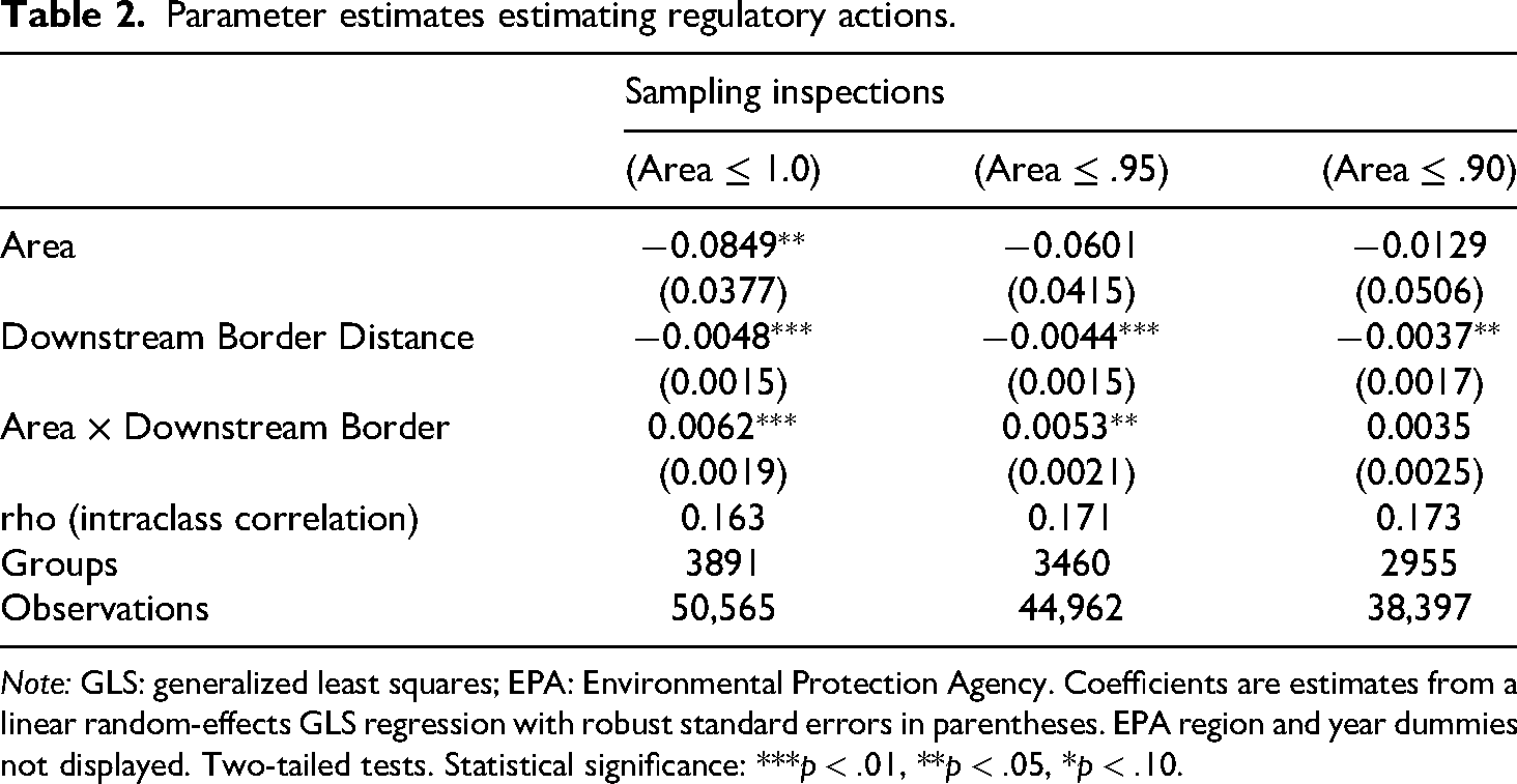
Note: GLS: generalized least squares; EPA: Environmental Protection Agency. Coefficients are estimates from a linear random-effects GLS regression with robust standard errors in parentheses. EPA region and year dummies not displayed. Two-tailed tests. Statistical significance: ***
Figure 6 displays the marginal effect of the proportion or area controlled over a facility’s distance from the closest downstream border. The plots illustrate how inspection effort varies over both having agency over one’s watershed and how close a facility is to a downstream border. When facilities are nearest a downstream border (the left side of the figures), the marginal effect of area is either negative or null, suggesting that increasing agency over the watershed either lowers or has no association with inspections or detection effort. The marginal effect of area however is positive for facilities that are sufficiently ’upriver’ from the nearest border. This is because agents can be held responsible for the effects that these facilities may have upon the local watershed. The right-hand side of the panels suggest that as facilities are located well-within the watershed, enhancing agent’s control over their watershed incentivizes them to exert greater detection effort. The substantive size of this effect ranges anywhere between 0.5 and 2 additional inspections per facility per year, depending upon the distance to the downstream border.
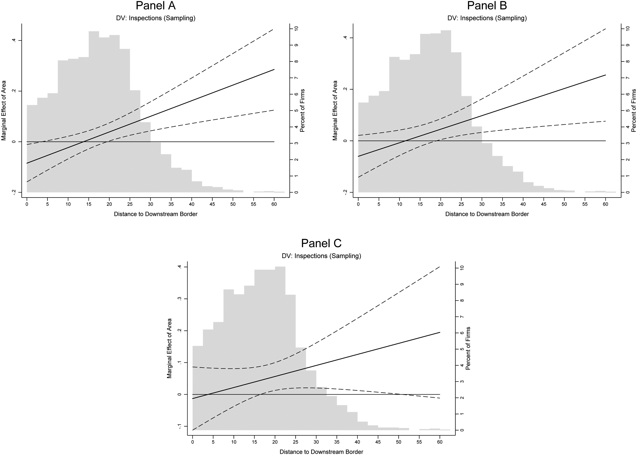
The marginal effect of the proportion of the watershed controlled over facility stream location by different enforcement outputs.
Policy scholars have long debated the merits of whether to devolve implementation authority to subunits. Our research underlines the value in considering how such devolution proceeds by highlighting how certain institutional designs may exacerbate public goods spillover in a policy arena. When devolution fragments a policy space, it induces joint policy-production relationships, where agents experience spillover of the public good being generated. To manage the tradeoffs inherent in such fragmented policy spaces, policy leaders must recognize the importance of not only the level and nature of fragmentation in the space, but also the distinct motivational levers at their disposal to reward agents’ private and public effort.
Our analysis expanded on prior literature by focusing on regulatory detection effort and incorporating the degree of resource fragmentation. The model reveals that regulatory effort varies across facilities based on their proximity to jurisdictional borders and the size of their jurisdiction. It provides valuable insights into the factors influencing regulators’ decision-making processes and highlights the role of network structures in shaping regulatory outcomes. If our account is correct, then we have preliminary evidence that under certain conditions regulatory detection effort is undersupplied, not due to the political demands of elected officials or local stakeholders, but because of the misaligned incentives that particular institutional configurations offer administrative agents. By addressing these gaps in the literature, our model identifies the factors that influence regulatory effort and the potential consequences of inadequate coordination and contributes to the broader understanding of effective governance and policy delivery.
Our paper’s contributions, while relevant to environmental pollution, are not limited to them. Our model can be extended to any context where a public good is delivered in an interrelated network that fragments a resource. Consider, for example, that in environmental applications, the relevant forcing variables that order the flow of effort is gravity with water pollution, or prevailing winds with air pollution. But the relevant forcing variable could take on different forms in other settings. For example, the forcing variable could also be time. Under this interpretation, we could imagine extensions to educational policy where resource fragmentation could present over grade levels (e.g. first grade, second grade, and third grade). In this application, teacher effort at a given level would be conditioned by the temporally upstream teacher effort provided at lower levels. Under yet another interpretation, the forcing variable could be geographic distance between neighborhoods. Under this interpretation, we can imagine extensions to home values where resource fragmentation could present as contiguous neighborhood boundaries. In this context, homeowner upkeep effort would be conditioned by the distance toward upstream homeowners’ effort provided in nearer neighborhoods. In short, we believe that our model’s potential applications are broad enough to provide insight into a host of alternative policy settings.
Our findings emphasize the importance of effective institutional design and coordination mechanisms in addressing the challenges posed by spillovers. Moving forward, policymakers and practitioners can draw valuable insights from this research to inform the design of more robust and efficient environmental governance systems. It emphasizes the need for policy interventions that address the challenges posed by spillovers and jurisdictional fragmentation. What might an ideal or optimal institutional design of state regional offices look like in the context of water pollution control? The answer to this question depends upon whether watershed dissection occurs across state lines or across regional boundaries within a state. When watersheds are dissected by state boundaries, the obvious solution is greater attention by the U.S. EPA—the natural hierarchical actor to resolve state-level cooperation dilemmas. When watersheds are dissected by regional boundaries within the state, our results suggest that intra-state regional office boundaries would do better to follow watershed boundaries rather than county boundaries, the current norm. Regional offices ought to overlap with their watersheds when possible, thereby reducing dissected watersheds and enhancing regional officers’ ownership over their resource. Another possibility, not pursued here but left to future work, is that state pollution control agencies may be able to mitigate intrastate cooperation problems by locating decision-making authority over enforcement activity at levels higher than the regional office. Such a nested hierarchical solution would incentivize a mid-level bureaucrat, with authority over competing regions, to intervene and resolve such cooperation dilemmas.
The model developed here also admits several implications that go beyond the tested hypotheses and may serve as a foundation for further work on boundary design. First, one can show that realigning regional office boundaries along watershed lines does not increase total enforcement effort in the aggregate: the equilibrium sum of provision across all regulators is invariant to how watershed-aligned boundaries are drawn. Boundary redesign redistributes enforcement burden—shifting costs onto whichever office holds downstream responsibility—rather than expanding effort overall. The inspection shortfalls documented above are therefore a symptom of misallocated burden, not of insufficient total effort; interventions that increase aggregate resources without addressing allocation may not resolve the underlying incentive problem. Second, the welfare case for consolidation is conditional: merger dominates fragmentation only when the cross-jurisdictional spillover rate exceeds a computable threshold that depends on the benefit function and equilibrium provision level. Below this threshold, fragmentation can be welfare-superior even in the presence of genuine spillovers, implying that the standard prescription to align office boundaries with watersheds is not universally correct. The empirical apparatus of the present paper—which identifies the magnitude of inter-jurisdictional spillover effects—provides the data required to evaluate whether observed spillovers clear this threshold. Third, for any politically-constrained map that cannot be redesigned, one can show that intergovernmental grants can substitute for boundary realignment at a calculable price, providing a direct fiscal benchmark for evaluating programs designed to compensate for boundary-induced enforcement gaps.
Supplemental Material
sj-pdf-1-jtp-10.1177_09516298261454888 - Supplemental material for Policy devolution and cooperation dilemmas
Supplemental material, sj-pdf-1-jtp-10.1177_09516298261454888 for Policy devolution and cooperation dilemmas by Robert J Carroll, David M Konisky, and Christopher Reenock in Journal of Theoretical Politics
Supplemental Material
sj-docx-2-jtp-10.1177_09516298261454888 - Supplemental material for Policy devolution and cooperation dilemmas
Supplemental material, sj-docx-2-jtp-10.1177_09516298261454888 for Policy devolution and cooperation dilemmas by Robert J Carroll, David M Konisky, and Christopher Reenock in Journal of Theoretical Politics
Footnotes
Acknowledgments
We gratefully acknowledge the support of National Science Foundation Grants SES-1425883 and SES-1551617 to allow us to conduct this research. We also thank Shannon Conley, Kevin Dyrland, Evan Linskey, and Joe Vukovich and for their valuable research assistance.
Funding
The authors received no financial support for the research, authorship, and/or publication of this article.
Declaration of conflicting interests
The authors declared no potential conflicts of interest with respect to the research, authorship, and/or publication of this article.
Supplemental material
Supplemental material for this article is available online.
Notes
References
Supplementary Material
Please find the following supplemental material available below.
For Open Access articles published under a Creative Commons License, all supplemental material carries the same license as the article it is associated with.
For non-Open Access articles published, all supplemental material carries a non-exclusive license, and permission requests for re-use of supplemental material or any part of supplemental material shall be sent directly to the copyright owner as specified in the copyright notice associated with the article.