Machine learning-based prediction of statically equivalent seismic forces in pin-supported cylindrical reticulated shells

Abstract

Reticulated shells exhibit complex vibrations during earthquakes, encompassing components in horizontal and vertical directions, and multiple vibration modes occur. In particular, single-layer reticulated shells with a small depth relative to their span exhibit many vibration modes, and the shapes of these modes can vary depending on the geometry. The method for rapidly setting equivalent static seismic forces remains unexplored. In response to the above background, this study proposes a novel approach for calculating the seismic forces on single-layer reticulated shells using machine learning techniques. The shells in focus are pin-supported cylindrical reticulated shells, typically for the roofs of gymnasiums used as evacuation facilities during severe earthquakes in Japan. Machine learning uses numerical analysis results for approximately 20,000 shells, with varied spans, half-open angles, and aspect ratios. A method for preprocessing the principal vibration modes as image data is proposed, after which the imaged vibration modes are predicted from the shape parameters of the shell using a neural network. The prediction accuracy is analyzed, and a method for rapidly calculating seismic loads based on combining predicted vibration modes is proposed. These seismic loads are compared with the response spectrum method results, and their effectiveness is discussed.

Keywords

Single-layer latticed shell cylindrical shell seismic response evaluation seismic force machine learning neural network

Introduction

Reticulated shells are roof structures covering large spaces, comprising linear members, such as steel arranged in a mesh, to form a curved surface. These structures require careful consideration of buckling behavior under self-weight or snow loads, and extensive research has been conducted to evaluate buckling strength.^1–3 Meanwhile, in regions prone to significant seismic activity, it is also necessary to consider to the unique response characteristics that differ from those of multistory buildings.^4,5 Reticulated shells can exhibit vertical responses to horizontal seismic motions. Additionally, in Japan, reticulated shells are evacuation facilities during earthquakes. However, buckling of members and damage to nonstructural components such as ceilings have been reported past earthquakes, undermining its usefulness as shelters.^6,7

In the seismic design of reticulated shells, response spectrum analysis, such as the CQC method,⁸ can accurately estimate the elastic seismic responses. It has been demonstrated that the strategy of inducing plasticization in the substructure to reduce the seismic forces transmitted to the shell is effective against extremely large seismic events.^9,10 However, it is crucial to determine the seismic forces explicitly to analyze the elastoplastic buckling behavior^11,12 during an earthquake or estimate the seismic performance using pushover analysis.

Ishikawa and Kato¹² and Yamada,¹³ describe the complex seismic response of a reticulated shell with many vibration modes. Their behavior is influenced by the supporting system, their geometries, and out-of-plane stiffness. Kato et al.¹⁴ highlighted the difficulty of formulating their statically equivalent seismic forces based on one mode, especially for single-layer spherical reticulated domes with thin depth. In contrast, they also mentioned that in the case of relatively thick depth, there is a possibility of expressing the seismic forces by using two modes as a vector form. They developed a two-mode-based approach to seismic loads in a vector form for a relatively thick spherical dome supported by a substructure,^15,16 extending their proposal of a response estimation method that considers plasticization of substructures. Takeuchi et al.¹⁷ showed that the number of primary vibration modes decreases as the ratio of the depth to the span of the shell supported by the substructure increases. Then, focusing on shells with large depths, they proposed an efficient equation to evaluate the equivalent static seismic load of the shell by organizing the effect of response amplification due to resonance of the substructure using the mass and natural period ratios. This method is extremely helpful in calculating acceleration distributions by hand and is used in the Japanese guidelines.¹⁸ The applicable range is a span–depth ratio of 1/50 or greater more for domes and 1/100 or greater for cylindrical shells. Nair et al.¹⁹ extended this method to the case in which a high-rise building supports dome. Also, Cedron et al.²⁰ have discussed methods of determining static seismic forces for arch structures. However, it remains challenging to define seismic loads for a shell as thin as a single-layer reticulated shell. Takiuchi et al.²¹ focused on the strain-energy ratio of the modes and highlighted the two-mode based seismic force is applicable for some free-form and peripherally pin-supported cylindrical shells. It still requires determining several hundred eigenvalues from which modal parameters must be analyzed, which is cumbersome procedure compared to thick shells.

The rapid progress of machine learning technology in recent years enables new approaches to predict such complex phenomena. In civil engineering structures, such as predicting vibration behavior²² and buckling loads in shell structures,²³ optimization²⁴ has also been conducted. However, in the context of statically equivalent seismic forces for reticulated shells, machine learning has not been widely applied.

With the above background, this study introduces the use of supervised learning with Convolutional Neural Networks (CNNs)²⁵ to rapidly predict vibration modes, significantly reducing the time required for eigenvalue analysis and subsequent modal analysis. The proposed method leverages the power of machine learning to achieve high accuracy, predicting vibration modes on test data.

This paper is structured as follows: Section 2 describes the dataset of cylindrical reticulated shells used in this study. Section 3 details the preprocessing method for converting vibration modes into image data and the architecture of the machine learning model. In Section 4, the numerical analysis results are presented and the accuracy of the model is discussed. Section 5 provides a summary of the findings and suggests potential directions for future research.

Structural models of the dataset

Structural model

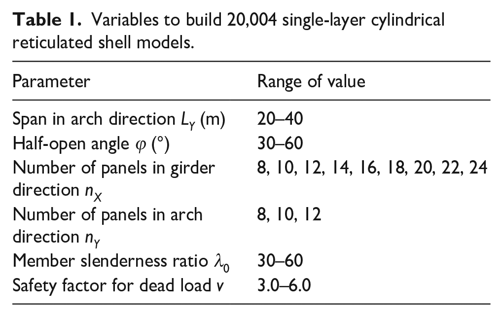
This investigation uses the parameters in Table 1 to generate 20,004 single-layer cylindrical reticulated shell models. In the generation process, structural parameters are defined by random sampling using uniform random numbers. Figure 1 shows the cylindrical reticulated shell’s basic shape. The shell has a rectangular plan, and the points on the peripheral boundary are pin-supported (Figure 2).

Table 1.

Variables to build 20,004 single-layer cylindrical reticulated shell models.

Parameter	Range of value
Span in arch direction L_Y (m)	20–40
Half-open angle ϕ (°)	30–60
Number of panels in girder direction n_X	8, 10, 12, 14, 16, 18, 20, 22, 24
Number of panels in arch direction n_Y	8, 10, 12
Member slenderness ratio λ₀	30–60
Safety factor for dead load v	3.0–6.0

Figure 1.

Basic shape of the cylindrical reticulated shell: (a) cylindrical shell and (b) tubular section.

Figure 2.

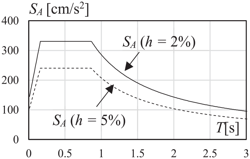
Acceleration response spectrum of input ground motions for serviceability limit level.

The structural network is a three-way grid member arrangement. Each structure comprises rigidly jointed tubular members. Young’s modulus E of the members is 205,000 N/mm², and the yield stress σ_y is 235 N/mm².

Each cylindrical shell comprises equilateral triangular panels, and the diameter D of the tubular section is determined by the fundamental length l₀, defined as the length of one side of the panel. Using the member slenderness ratio λ₀ in Table 1, the diameter D is assumed by equation (1),

D = 2 \sqrt{2} \frac{l_{0}}{λ_{0}}

(1)

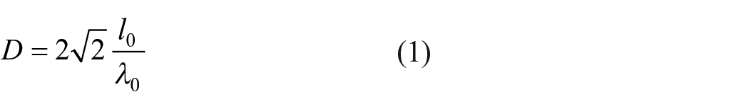
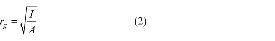
where the value λ₀ is defined by using the radius of gyration member r_g based on sectional area A and second moment of inertia I.

r_{g} = \sqrt{\frac{I}{A}}

(2)

Within each structure, the same D is applied to all members. The member thickness t of the tubular member is assumed such that each structure satisfies the ultimate strength under the dead load with a load factor v (safety factor). Table 1 shows that the value of v ranges from 3.0 to 6.0. Because this type of structure is known to be sensitive to buckling, the cross section should be designed so as not to include shells with too low or too high buckling resistance in the data set. This research adopts the method described in the IASS WG 8,⁴ and Nakazawa et al.,⁵ the ultimate strength of cylindrical reticulated shells while considering buckling characteristics. The methodology of this study is briefly described as follows.

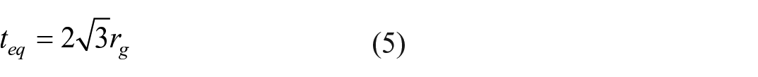
The shell analyzed is initially assumed to comprise a common member with an initial wall thickness t_ini. Second, the linear buckling load P^lin is obtained from an eigenvalue analysis that considers geometric stiffness. Then, the value of the knockdown factor α₀ is introduced to estimate its elastic buckling load P^el considering the imperfection sensitivity. Accordingly, the elastic buckling load P^el is evaluated using equation (3), where the value of the knockdown factor α₀ is assumed using equation (4), based on Kato et al.²⁶ for the pin-supported cylindrical shell.

P^{e l} = α_{0} P^{l i n}

(3)

α_{0} = 0.706 \exp {- 0.621 w_{i 0} / t_{e q} + 0.081 (w_{i 0} / t_{e q})}

(4)

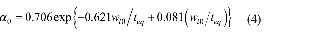
In equation (4), w_i₀ and t_eq are the imperfection amplitude and the equivalent shell thickness, respectively. According to the recommendation,^1,18 the value t_eq is evaluated using equation (5), and the value w_i₀ is assumed as 0.2t_eq. The value of α₀ used in this study is 0.63 from the above assumptions.

t_{e q} = 2 \sqrt{3} r_{g}

(5)

Load condition

The dead load, including member weight and roof finishing materials, is assumed to be uniformly distributed at 1.0 kN/m². The nodes are affected by the dead load, determined by the area of the equilateral triangles that make up the cylindrical shell.

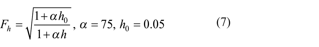
The design spectrum specified by Notification No.1457 of the Japan Building Code,²⁷ corresponding to the soil layer for medium soil type II, is adopted for response spectrum analysis and calculation of the seismic loads described below. The design spectrum S_A is given by equation (6), where F_h is the reduction factor reflecting the equivalent damping factor h, and G_S is the amplification factor due to soil Type II. This study assumes equation (7) for the reduction factor F_h.

S_{A} = S_{A 0} (T) F_{h} (h) G_{s} (T)

(6)

F_{h} = \sqrt{\frac{1 + α h_{0}}{1 + α h}}, α = 75, h_{0} = 0.05

(7)

The seismic input is assumed to be in the Y-direction because the direction of the arch of the cylindrical shell should cause a more complex response than seismic input in the X-direction. This study discusses the vertical response to horizontal seismic inputs is discussed in this study; however, ignores vertical seismic inputs. The combined response is a future issue due to simultaneous horizontal and vertical inputs.

Machine learning-based prediction of vibration modes

Two-mode-based seismic load

This study adopts the equivalent seismic loads of equation (8), where β_i and u_i represent the participation factor and vibration mode vector of the i-th mode, respectively. Here, M denotes the mass matrix, and η₁ and η₂ are the coefficients of the modal loads.

\begin{array}{l} P_{1} = η_{1} S_{A} (T_{i}, h) β_{i} M u_{i} + η_{2} S_{A} (T_{j}, h) β_{j} M u_{j} \\ P_{2} = η_{1} S_{A} (T_{i}, h) β_{i} M u_{i} - η_{2} S_{A} (T_{j}, h) β_{j} M u_{j} \end{array}

(8)

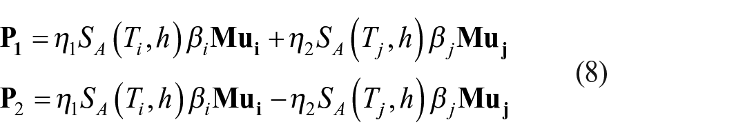
In this study, the η₁ and η₂ values are assumed to be 1.0. These coefficients vary depending on the importance of the mode. For example, if the shell is extremely dominant for the i-th mode, η₂ approaches 0. Further research is needed to determine appropriate η₁ and η₂ values.

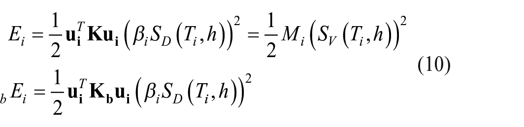
Kato and Nakazawa,¹⁴ Kato et al.,^15,16 Takiuchi et al.²¹ depicted that the two-mode seismic loading equation in equation (8) applies when the modal parameters of the shell structure satisfy equation (9). In the equation, ε_k is the strain energy ratio, and _bε_k is the bending strain energy ratio of the k-th vibration mode. The i-th and j-th vibration modes in equation (8) are recommended as the two modes with the largest ε_k. The strain energy ratio ε_k and the bending strain energy ratio _bε_k of the k-th mode are calculated using the following equations.²

\begin{array}{l} ε_{i} + ε_{j} \geq 0.8 \\ {{}_{b}ε}_{i} + {{}_{b}ε}_{j} \geq 0.2 \end{array}

(9)

\begin{array}{l} E_{i} = \frac{1}{2} u_{i}^{T} K u_{i} {(β_{i} S_{D} (T_{i}, h))}^{2} = \frac{1}{2} M_{i} {(S_{V} (T_{i}, h))}^{2} \\ {{}_{b}E}_{i} = \frac{1}{2} u_{i}^{T} K_{b} u_{i} {(β_{i} S_{D} (T_{i}, h))}^{2} \end{array}

(10)

\begin{array}{l} ε_{i} = E_{i} / \sum_{k = 1}^{N} E_{k} \\ {{}_{b}ε}_{i} = {{}_{b}E}_{i} / \sum_{k = 1}^{N} E_{k} \end{array}

(11)

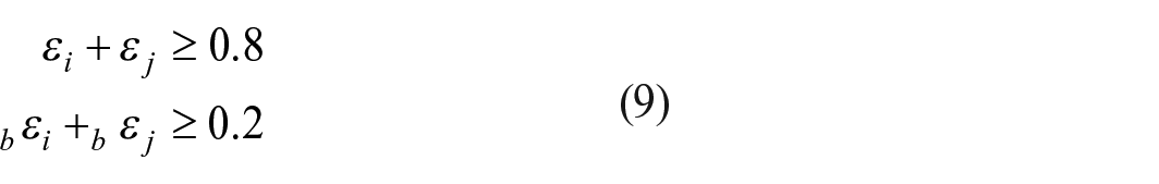
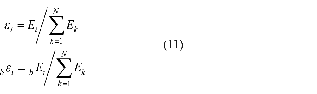
In equation (11), N is the number of vibration modes to consider, K is the stiffness matrix, and K_b is the stiffness matrix that ignores the axial stiffness of the member. In Takiuchi et al.²¹ N is determined so that the sum of the effective mass ratios ρ_k of each mode exceeds 90%, indicating that N could be in the hundreds, depending on the structure’s degrees of freedom of the structure.

Two modes will be selected based on the descending order of strain energy, with the mode exhibiting the longer natural period designated as Mode A and the one with the shorter period designated as Mode B. The subscripts A or B for modal parameters, such as natural periods (T_A and T_B), strain energy ratios (ε_A and ε_B), and effective mass ratios (ρ_A and ρ_B), indicates the parameters corresponding to Modes A and B, respectively. Previous study²¹ shows that structural parameters, such as half open angle, can change the shape of vibration modes and the balance between the two modes of the strain-energy ratio. Therefore, to ensure uniformity within the dataset, the dataset is generated so that the distribution of the difference between the strain energy ratios of Mode A and Mode B is uniform.

Conversion of vibration modes to image data

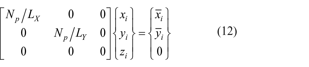
The vibration mode u_i of a structure is a data vector proportional to its degrees of freedom. Consequently, the data length of vibration modes varies depending on the structure. This study proposes preprocessing vibration modes as image data for machine learning. The vibration mode imaging allows the number of elements in the input layer of an ANNs to be kept constant for structures with different degrees of freedom. This preprocessing also permits using CNNs, which are widely used in the field of image recognition.

The image data uses the RGB color format, where each pixel represents a color with three elements: red, green, and blue. Let N_p be the number of pixels in the model image in terms of height and width; one vibration mode stores data in a 3D array of N_p × N_p × 3 (red, green, blue). In this study, the number of pixels, N_p is fixed to 50 based on a preliminary analysis. The X component of the vibration mode corresponds to the red of a pixel, the Y component to the green, and the Z component to the blue. The node i of the structure with coordinates {x_i, y_i, z_i} is transformed to coordinates { ${\bar{x}}_{i}$ , ${\bar{y}}_{i}$ } in the images as in equation (12). The origin of the coordinate system in the image is the lower-left corner of the image as shown in Figure 3.

[\begin{matrix} N_{p} / L_{X} & 0 & 0 \\ 0 & N_{p} / L_{Y} & 0 \\ 0 & 0 & 0 \end{matrix}] {\begin{matrix} x_{i} \\ y_{i} \\ z_{i} \end{matrix}} = {\begin{matrix} {\bar{x}}_{i} \\ {\bar{y}}_{i} \\ 0 \end{matrix}}

(12)

Figure 3.

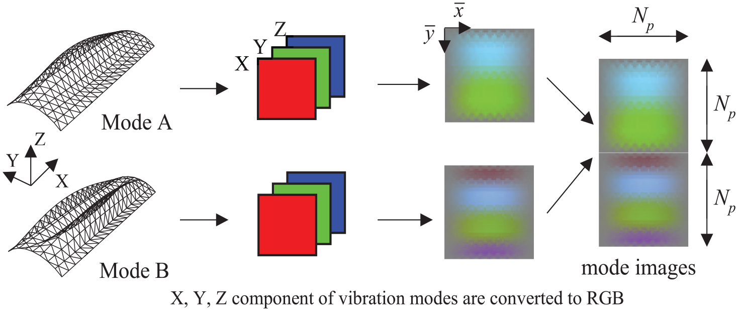
Conversion of vibration mode to image.

where L_X and L_Y in equation (12) are the spans in the X- and Y-directions, respectively. By comparing the coordinates of the pixel’s center with those of the structure’s node modified and projected using equation (12), the color of each pixel in the image represents the vibration mode component of the closest node. From equation (12), the transformation to the mode image is an affine transformation of the planar shape of the rectangular shell to an N_p × N_p square, and the z-direction coordinates of the shell are ignored. This method was adopted because of the shallow shells used in this study. As a preliminary study, the degree of information loss from converting vibration modes from natural vibration analysis to images and then from images back to vibration modes is examined. As a result, it is found that the conversion of shells with a large rise, such as 90° half-open angle, results in a loss of information, while the conversion and inverse conversion of shells with a half-open angle of 30° to 60°, the target of this study, can be done completely without any loss of information.

The imaging operation is performed separately for Modes A and B, and the results are concatenated vertically, as shown in Figure 3. This process transforms the two principal vibration modes of a single shell into data with dimensions N_p × 2N_p × 3. Note that the data for images, such as those shown in Figure 3, is in RGB color format; therefore, it must be stored as integer values from 0 to 255. However, the machine learning analysis described below uses real 3D array data (N_p × 2N_p × 3) calculated from the vibration mode values.

The image predicted by machine learning is then split into images of size N_p × N_p × 3 and used as the predicted value for each mode image. The mode image contains information on the X, Y, and Z components of the vibration modes of the structure, but not the rotational displacement components of the nodes. Then, the rotational component Θ is calculated using the translational component U of the mode according to equation (13).

\begin{array}{l} ω_{i}^{2} M {\begin{matrix} U \\ Θ \end{matrix}} = K {\begin{matrix} U \\ Θ \end{matrix}} = [\begin{matrix} K_{11} & K_{12} \\ K_{21} & K_{22} \end{matrix}] {\begin{matrix} U \\ Θ \end{matrix}} \\ Θ = - K_{22}^{- 1} K_{21} U \end{array}

(13)

where K₁₁, K₁₂, K₂₁, and K₂₂ represent the partial stiffness matrices corresponding to displacements (U ) and rotations (Θ). M is considered as a lumped mass matrix.

Image prediction

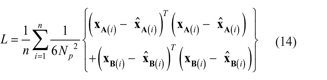
This study predicts the mode images using the ANNs depicted in Figure 4. The input layer of the network comprises three nodes, corresponding to aspect ratio α, depth-span ratio D/L_Y, and half-open angle ϕ. The first five layers of hidden units are fully connected, after which the transposed convolution and upsampling layers used for image generation transform the input data. The Rectified Linear Unit (ReLU) functions²⁸ are used to activate all the coupled and transposed convolution layers of the hidden layer. The loss function is the mean squared error in equation (14).

L = \frac{1}{n} \sum_{i = 1}^{n} \frac{1}{6 {N_{p}}^{2}} {\begin{cases} {(x_{A (i)} - \hat{x_{A (i)}})}^{T} (x_{A (i)} - \hat{x_{A (i)}}) \\ + {(x_{B (i)} - \hat{x_{B (i)}})}^{T} (x_{B (i)} - \hat{x_{B (i)}}) \end{cases}}

(14)

Figure 4.

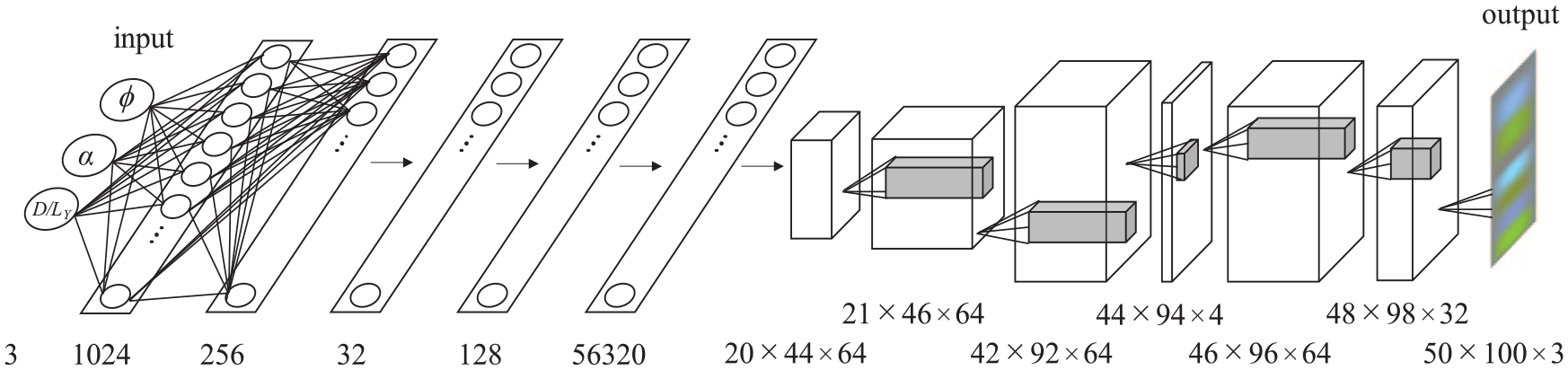
The architecture of a neural network for predicting dominant vibration modes.

where x_A_(i) and x_B_(i) are 3N_p² long vectors containing the values of the image elements corresponding to Modes A and B of the i-th shell in the training dataset, respectively, and ${\hat{x}}_{A (i)}$ and ${\hat{x}}_{B (i)}$ are their predicted values. Adam²⁸ was used to optimize the loss function with a learning rate of 0.001. As shown in Figure 4, the initial architecture comprises five fully connected layers in the hidden layer segment, with 1024, 256, 32, 128, and 56,320 node counts. Subsequently, the data from the fully connected layers are transformed into 3D tensor format. The configuration of the hidden layers, including number of layers, nodes, filters, and batch size was optimized through a hyperparameter search conducted using Optuna.²⁹

Results of numerical analysis

Prediction accuracy by machine learning

In this study, the generalization ability of machine learning models is assessed using k-Fold cross-validation. This method entails partitioning the dataset into k distinct subsets. During each validation cycle, a single subset is employed as the validation dataset, and the combination of the remaining k − 1 subsets serves as the training dataset. This training and evaluation process is iteratively conducted k times, with each of the k subsets being utilized as the test dataset precisely once. This systematic approach facilitates a thorough evaluation of the model’s performance, ensuring a comprehensive understanding of its generalization potential. During the k-fold cross-validation process, 18,000 out of 20,004 data points were utilized for training, focusing on optimizing hyperparameters for generalization performance. The remaining 2004 instances were reserved as the test dataset and were not used at any point during the training process. The model was re-trained on 18,000 training instances using the optimal hyperparameter configuration detailed in Section 3.3. This chapter discusses the prediction accuracy of the resulting trained model when applied to the test dataset.

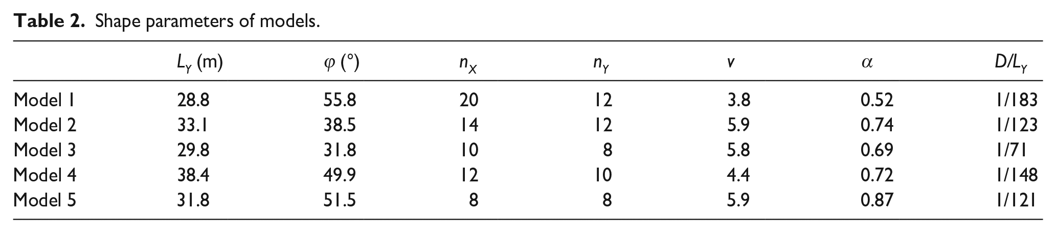
It is challenging to present the predicted vibrational characteristics of 2004 data points of test dataset within the confines of this paper. Therefore, five shells were selected, including those with high and low accuracies in predicting vibrational modes by machine learning, designated as Models 1–5. These models were comprehensively selected from an analysis of 2004 data to illustrate typical regression successes and failures. Similar trends to these five cases have been observed in other instances of test data that cannot be included in the manuscript. Table 2 details the shape parameters of Models 1 to 5. Figure 5 illustrates the shapes and modal parameters of Modes A and B for the four shells (Table 3).

Table 2.

Shape parameters of models.

	L_Y (m)	ϕ (°)	n_X	n_Y	v	α	D/L_Y
Model 1	28.8	55.8	20	12	3.8	0.52	1/183
Model 2	33.1	38.5	14	12	5.9	0.74	1/123
Model 3	29.8	31.8	10	8	5.8	0.69	1/71
Model 4	38.4	49.9	12	10	4.4	0.72	1/148
Model 5	31.8	51.5	8	8	5.9	0.87	1/121

Figure 5.

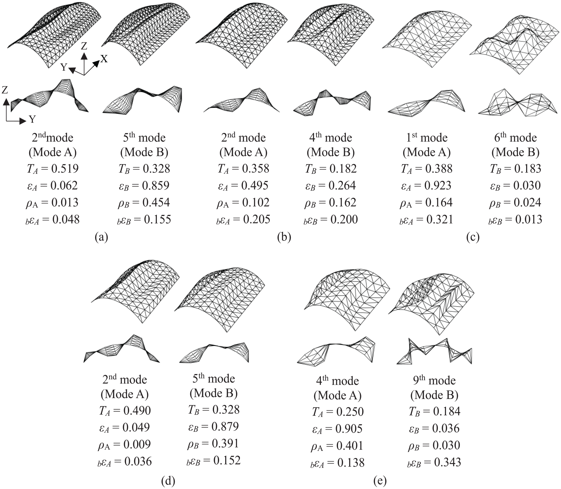
Dominant vibration mode diagrams and modal parameters for each model: (a) Model 1, (b) Model 2, (c) Model 3, (d) Model 4, and (e) Model 5.

Table 3.

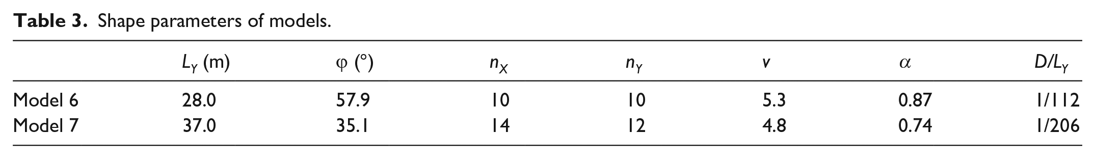
Shape parameters of models.

	L_Y (m)	ϕ (°)	n_X	n_Y	v	α	D/L_Y
Model 6	28.0	57.9	10	10	5.3	0.87	1/112
Model 7	37.0	35.1	14	12	4.8	0.74	1/206

As illustrated in Figure 5, Models 1 and 4 exhibit strain energy ratios ε_B for Mode B exceeding 0.8, whereas the strain energy ratio for Mode A of Models 3 and 5 exceeds 0.9. Consequently, it was inferred that a single mode predominated in Models 1, 3, 4, and 5. In contrast, Model 2 is characterized by closely aligned strain energy ratios across the two modes.

Figure 6 compares the results of converting the modes in Figure 5 into mode images and the mode images predicted by machine learning with ANNs. As shown in Section 3.3, modes A and B images are combined vertically during training and prediction. Figure 6, modes A and B images are shown separately for the reader's viewing convenience. The black line in Figure 6 shows the vibration modes obtained from the analysis, and the red line is the inverse transform of the image predicted by machine learning. Hereafter, the vibration mode calculated based on the mode image output of the ANNs is referred to as the predicted mode ${\hat{u}}_{A}, {\hat{u}}_{B}$ .

Figure 6.

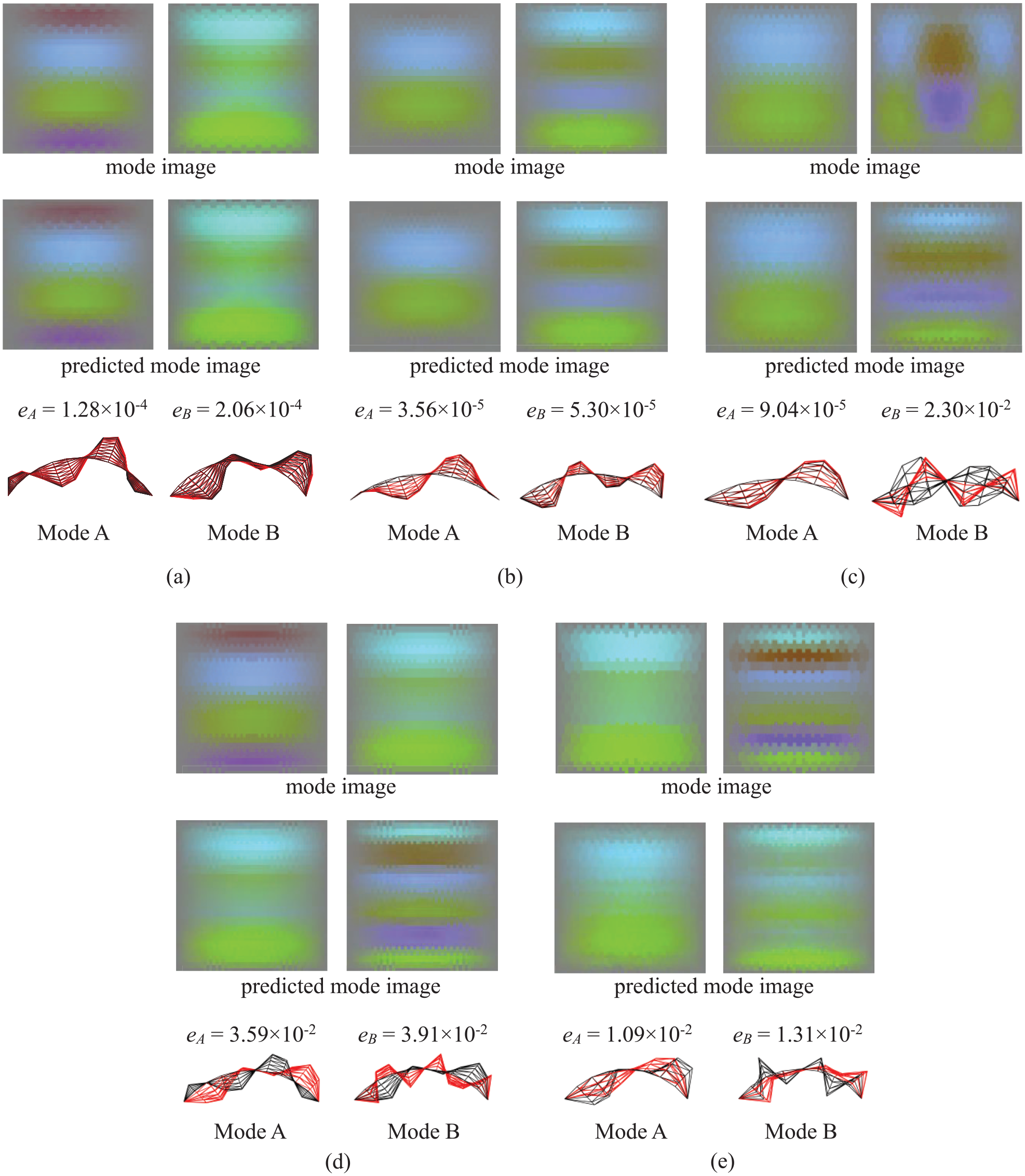
Comparisons between dominant vibration modes and their predicted modes across five models: (a) Model 1, (b) Model 2, (c) Model 3, (d) Model 4, and (e) Model 5.

To analyze the accuracy of the predicted modes, the following error function e_A and e_B are introduced using the image vector x_A, x_B of the vibration mode and the image vector ${\hat{x}}_{A}, {\hat{x}}_{B}$ of the prediction mode.

\begin{array}{l} e_{A (i)} = \frac{1}{3 {N_{p}}^{2}} {(x_{A (i)} - \hat{x_{A (i)}})}^{T} (x_{A (i)} - \hat{x_{A (i)}}) \\ e_{B (i)} = \frac{1}{3 N_{p}^{2}} {(x_{B (i)} - \hat{x_{B (i)}})}^{T} (x_{B (i)} - \hat{x_{B (i)}}) \end{array}

(15)

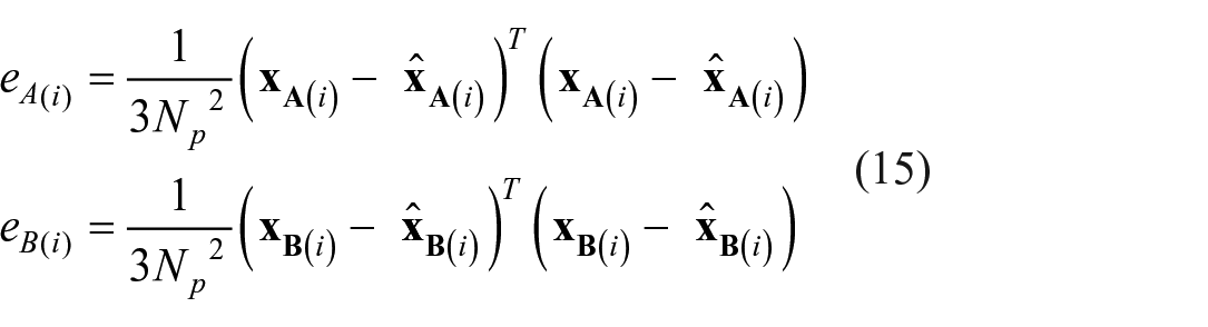
As previously mentioned in Section 3.2, the vibration modes can be accurately recovered from the mode images for the shells covered in this study. Therefore, the values e_A and e_B are indicators of how closely the predicted vibration modes match those obtained from natural vibration analysis. The closer values e_A and e_B are to zero, the more accurately the vibration modes are predicted.

From the analysis of the figures, it is clear that Models 1 and 2 can accurately predict the shapes of Modes A and B. In contrast, Model 3 accurately predicts Mode A but fails to predict Mode B. Model 4 significantly differs between the predicted and actual vibrational modes for Modes A and B. However, for Model 4, the shape of the predicted Mode A closely aligns with that of Mode B from the analytical results, as illustrated in Figure 7. Model 5 exhibits poor prediction accuracy for both modes, with a particularly low accuracy in predicting the amplitude at the roof apex for Mode A.

Figure 7.

Model 4 Mode B (black line) compared to predicted Mode A (red line).

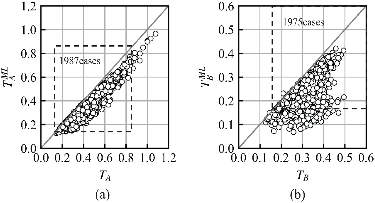
Figure 8 presents scatter plots of the values of e_A and e_B for the 2004 test data points. The horizontal axis of this graph represents the difference in strain energy ratios between Modes A and B. The prediction error e_A and e_B for the test data are distributed below 1.0 × 10⁻³, in many cases, encompassing Mode A of Models 1, 2, and 3, and Mode B of Models 1 and 2.

Figure 8.

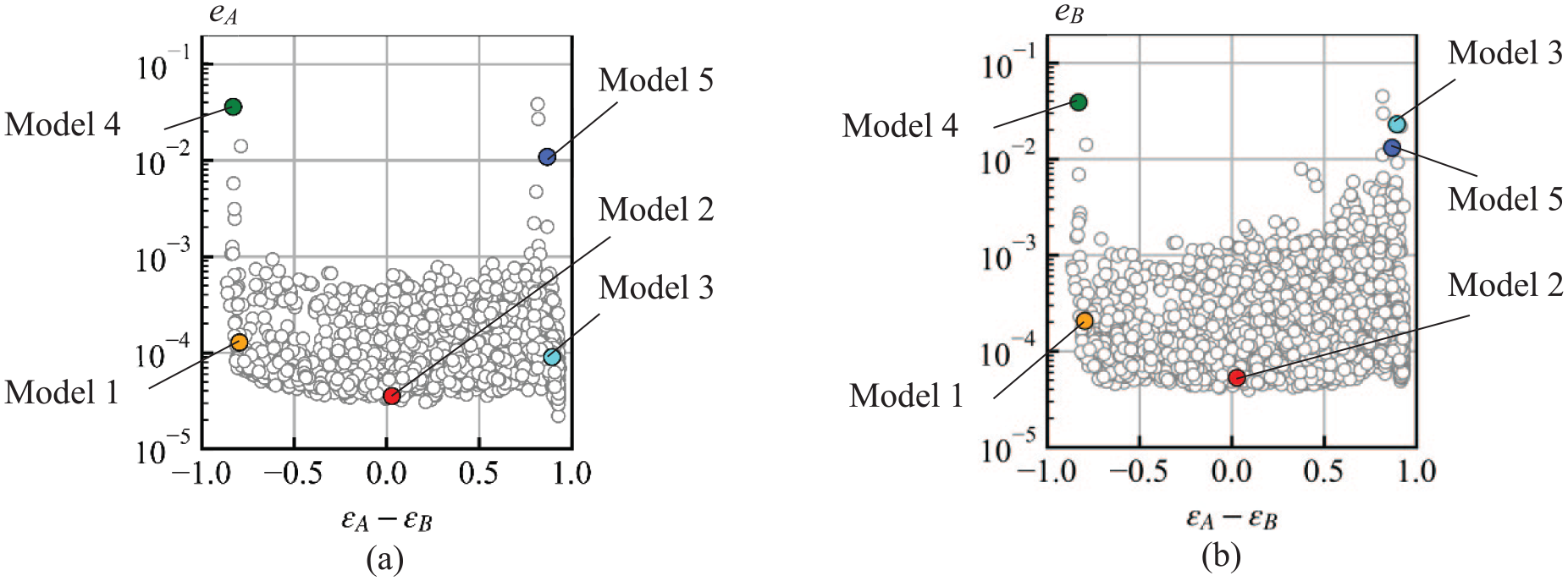
Scatter plots of the values of e_A and e_B for 2004 test data points: (a) Mode A and (b) Mode B.

In the scatter plot of Figure 8, a trend can be observed where cases with prediction errors greater than 1.0 × 10⁻³ are distributed in areas with large differences in strain energy ratios on the left and right sides, indicating instances where one mode becomes dominant. Figure 9 shows the shape of the vibration modes near e_A = 1.0 × 10⁻³. The figure shows that the predicted mode in red and the vibration mode in black are generally of the same shape. As shown in Figure 5, in the case of a successful prediction, the error function e_A is 1.28 × 10⁻⁴ for Mode A of Model 1, which is smaller than 10⁻³. Similarly, for Mode A of Model 4, e_A is 3.59 × 10⁻². Conversely, when the prediction clearly fails, as can be seen visually, the values of e_A and e_B are even larger.

Figure 9.

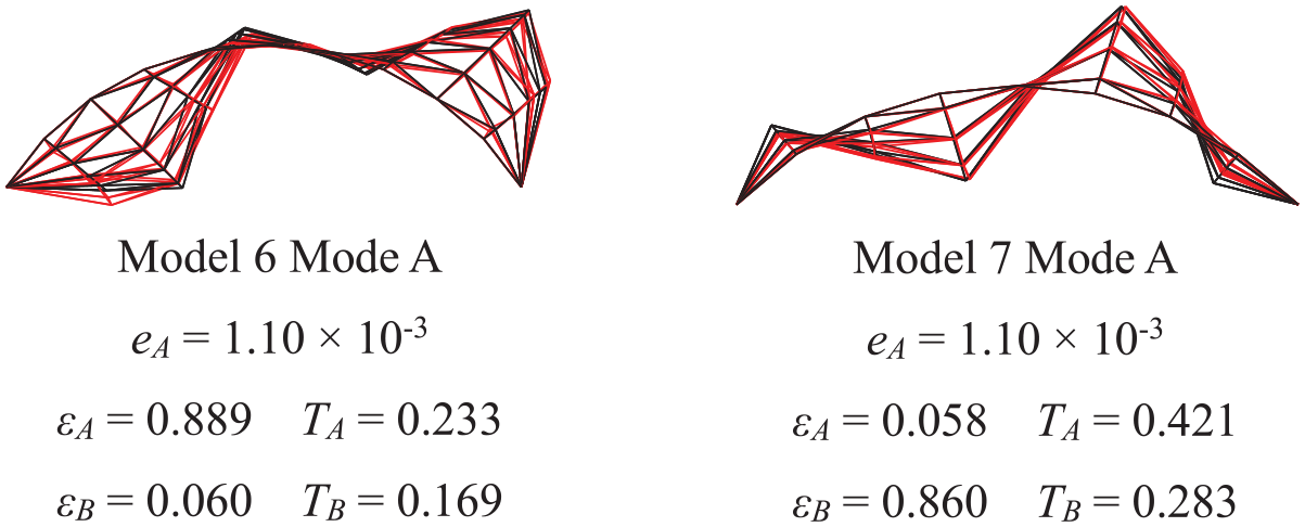
Models 6, 7 that e_A ≃ 1.00 × 10⁻³. Mode A (black line) compared to predicted Mode A (red line).

Out of 2004 test data, 1987 models have e_A of less than 1.0 × 10⁻³, and 1845 models have e_B of less than 1.0 × 10⁻³. The ANNs could predict approximately 99 and 92% of the modes A and B in the test dataset. One possible reason for the lower regression accuracy for Mode B compared to Mode A is that Mode B has shorter natural periods and more complex mode shapes than Mode A. In Figure 5, Mode A is limited to waves with number of half-wavelength numbers of 2 or 4, while Mode B includes mode shapes such as Model 3, which has waves in the X direction, and Model 5, which has a larger number of waves, in addition to Mode A-like shapes. This tendency for Mode B to exhibit a greater variety of mode shapes is confirmed throughout the data set.

Focusing on individual models, Mode A of Models 4 and 5 and Mode B of Models 3, 4, and 5 fall within the range of poor prediction accuracy. Meanwhile, Model 1 has good accuracy for both Modes A and B, and Model 3 has good accuracy for one of both. Model 4 also predicts true Mode B as Mode A. From Figures 6 to 8 show that the prediction accuracy deteriorates when there is a significant difference in the strain energy ratio between Modes A and B, indicating failures in predicting modes with lower strain energy ratios. Additionally, there are instances, such as in Model 5, where predictions fail for both modes, but such cases are very rare within the test data.

Prediction of natural periods of principal modes

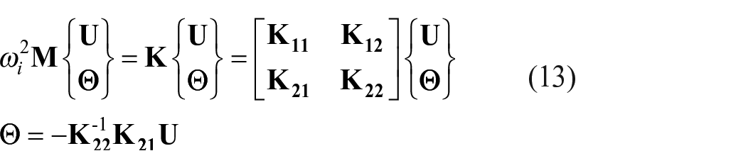
In this study, the rotational component of the mode is derived from the vibrational mode predicted using equation (13). Subsequently, the natural periods ( $T_{A}^{M L}$ and $T_{B}^{M L}$ ) are estimated using equation (16).

\begin{array}{l} {(ω_{A}^{M L})}^{2} = \frac{{\hat{u}}_{A}^{T} K {\hat{u}}_{A}}{{\hat{u}}_{A}^{T} M {\hat{u}}_{A}}, {(ω_{B}^{M L})}^{2} = \frac{{\hat{u}}_{B}^{T} K {\hat{u}}_{B}}{{\hat{u}}_{B}^{T} M {\hat{u}}_{B}} \\ T_{A}^{M L} = \frac{2 π}{ω_{A}^{M L}}, T_{B}^{M L} = \frac{2 π}{ω_{B}^{M L}} \end{array}

(16)

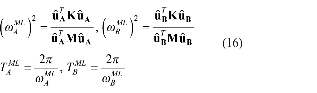
Figure 10 shows accuracy of the natural period evaluation, which includes plots for the 2004 shells of the test dataset. Generally, for Modes A and B, the estimated natural periods were lightly shorter than the actual natural period in most instances. Additionally, the variability in the prediction accuracy was more pronounced for Mode B than for Mode A. This discrepancy in prediction accuracy between the modes, as illustrated in Figure 8, might contribute to the greater variability observed for Mode B. However, the values of the acceleration response spectra in Figure 2 are constant between 0.16 and 0.86 s, indicating that the impact of this natural period prediction error on the seismic load calculation is limited. The reason why $T_{A}^{M L}, T_{B}^{M L}$ calculated by equation (16) from the predicted modes were evaluated to be shorter than T_A, and T_B is the prediction accuracy of the vibration modes. Another reason could be that the predicted modes do not satisfy their orthogonality. Improvement of this point remains an issue for future research.

Figure 10.

Comparisons of natural periods calculated from natural vibration analysis and predicted values: (a) Mode A and (b) Mode B.

Seismic loading with predicted modes

The calculation of the two-mode seismic load formula, as shown in equation (8), uses the natural periods ( $T_{A}^{M L}, T_{B}^{M L}$ ) and participation factor ( $β_{A}^{M L}, β_{B}^{M L}$ ) derived from the predicted modes ( ${\hat{u}}_{A}, {\hat{u}}_{B}$ ), following the methodology outlined in equation (16). Figure. 11 compares responses from this two-mode seismic load with those obtained using the CQC method. The responses illustrated in the figure exclude components due to dead loads. The bending moment M is calculated as the square root of the sum of the squares of the bending moments M_y and M_z, corresponding with the bending moments about the y- and z-axes, respectively, when the member longitudinal axis is aligned with the x-axis. From Figure 11, it is evident that Models 1 and 2, which accurately evaluated both Modes A and B, generally correspond to the predictions made using the CQC method, indicating their capability to determine the seismic load that can produce such predictions. Due to the setting of η to 1.0 in equation (8), it is observed that the seismic loads applied to Model 2, which considers the effects of two modes, tend to slightly overestimate the seismic responses compared to those applied to Model 1. Similarly, Models 3 and 4, which effectively evaluates a single dominant mode, enables precise response assessments under seismic loading. Even Model 5, which shows poor predictive accuracy for both Modes A and B, can still achieve a conservative response evaluation by summing up the modes with η set to 1.0. However, this model also exhibits the largest variation in predictive accuracy among all models.

Figure 11.

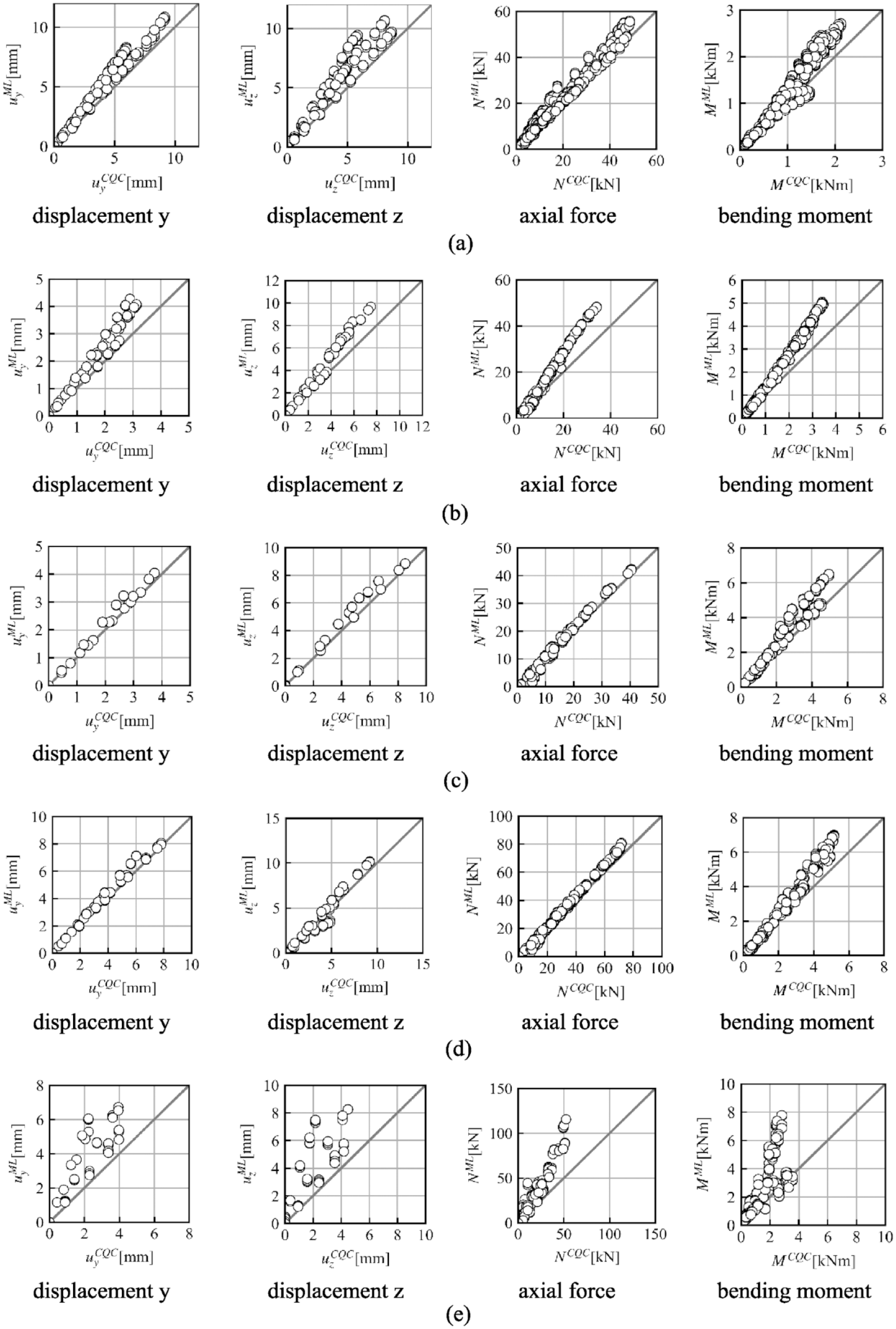
Comparison of responses due to the two-mode-based statically seismic forces with those obtained by the CQC method: (a) Model 1, (b) Model 2, (c) Model 3, (d) Model 4, and (e) Model 5.

Conclusions

This paper evaluated the simplified seismic loads of single-layer cylindrical lattice shells characterized by a low depth-to-span ratio. A method proposed in prior research was adopted to construct seismic loads through the superimposition of two dominant vibrational modes, Modes A and B. Using dataset of approximately 20,000 cylindrical reticulated shells with pin-supported boundaries, a preprocessing method to convert vibration modes into images, and a machine learning method to predict the primary vibration modes from the geometry of the cylindrical shell were proposed. This paper draws the following conclusions:

(1) Among the 2004 test datasets not used for ANNs training, the error function e_A and e_B, serving as a threshold value of 0.001, was observed to fall below this threshold in predicting the general shape of vibration Modes A and B in over 90% of the cases. The prediction was based on the half-open angle, aspect ratio, and span-to-depth ratio of the input data. The value of e_A distributed between 2.21 × 10⁻⁵ to 3.83 × 10⁻², the value of e_B ranged from 3.95 × 10⁻⁵ to 4.48 × 10⁻².

(2) Three patterns were observed in cases of poor prediction accuracy of the mode images: (i) one dominant mode is predicted successfully, whereas the prediction fails for the second mode with smaller strain energy; (ii) Mode A is incorrectly predicted as Mode B, effectively reversing them; and (iii) predictions fail for both modes. Prediction accuracy decreases notably when there is a significant difference in the strain energy between Modes A and B.

(3) Based on the predicted vibration modes, the evaluated natural periods tended to be slightly shorter than the actual natural periods. This tendency is more pronounced for Mode B. In the case of the dataset in this study, more than 90% of the evaluated values of natural periods are in the constant acceleration region of the design spectrum; therefore, their influence on the seismic load evaluation is limited. Improving the accuracy of this evaluation is identified as a future task.

(4) Even in Model 5, where the prediction accuracy of the two modes is the poorest, the equivalent static seismic force based on the two predicted modes is evaluated on the safe side compared to the response using the CQC method.

This study focused on the primary dominant vibrational modes of cylindrical lattice shells supported by pin boundaries. The mode-response amplification, due to the shell being supported by a substructure, varies with the mass and period ratios between the shell and the substructure. Using two-mode seismic loads in cases in which a substructure supports the shell remains challenging for future research. Furthermore, the shape of the dominant vibrational modes changes with variations in the shape of the shell and support conditions. Therefore, the results of this study are limited to pin-supported shell boundaries, and the prediction of vibration modes for cylindrical shells with roller support or different support configurations with free boundary edges is a future issue.

Footnotes

Declaration of conflicting interests

The author(s) declared no potential conflicts of interest with respect to the research, authorship, and/or publication of this article.

Funding

The author(s) received no financial support for the research, authorship, and/or publication of this article.

ORCID iD

Yuji Takiuchi

References

IASS WG 8. Guide to buckling load evaluation of metal reticulated roof structures. Report of activities IASS WG8. International Association of Shell and Spatial Structures, Spain, 2014.

Kato

Fujimoto

Ogawa

Buckling load of steel single-layer reticulated domes of circular plan. J Int Assoc Shell Spat Struct 2005; 46: 41–63.

Bulenda

Knippers

Stability of grid shells. Comput Struct 2001; 79(12): 1161–1174.

IASS WG 8. Guide to earthquake response evaluation of metal reticulated roof structures. Report of Activities IASS WG8. International Association of Shell and Spatial Structures, Spain, 2019.

Nakazawa

Kato

Takeuchi

, et al State-of-the-art of seismic response evaluation methods for metal roof spatial structures. J Int Assoc Shell Spat Struct 2012; 53: 117–130.

Kawaguchi

. Damage to non-structural components in large rooms by the Japan earthquake. In: Structures congress 2012, Chicago, United States, 2012, pp.1035–1044. DOI: 10.1061/9780784412367.

Sasaki

Aoi

Kajiwara

, et al Collapse mechanism of wide-area suspended ceiling in school gymnasium. In: Proceedings of IASS annual symposia, Boston, United States, July 2018, pp.1–7.

Wilson

Der Kiureghian

Bayo

EP.

A replacement for the SRSS method in seismic analysis. Earthquake Eng Struct Dyn 1981; 9(2): 187–192.

Kato

Takiuchi

Keisuke

, et al Effectiveness of buckling restrained braces for upgrading earthquake resistant capacity of single layer grid dome. Eng Struct 2022; 261: 114280.

10.

Takiuchi

Kato

Nakazawa

, et al Earthquake response evaluation of cylindrical latticed shell roofs supported by BRBs Comparison of responses based on Chinese codes and Japanese regulations. Int J Space Struct 2024; 39(1): 21–35.

11.

Ogawa

Takeuchi

Kumagai

, et al Buckling loads of single layer lattice domes under antisymmetric loading. J Struct Eng 2013; 59: 463–469. (in Japanese)

12.

Ishikawa

Kato

Elastic-plastic dynamic buckling analysis of reticular domes subjected to earthquake motion. J Space Struct 1997; 12: 3–4.

13.

Yamada

Vibration behaviour of single-layer latticed cylindrical roofs. Int J Space Struct 1997; 12: 181–190.

14.

Kato

Nakazawa

. Seismic design method to reduce the responses of single layer reticular domes by means of substructure under severe earthquake motions. In: Proceedings of IASS 2001 Symposium Nagoya, Nagoya, Japan, 2001, TP.077.

15.

Kato

Nakazawa

Saito

Estimation of static seismic loads for latticed domes supported by substructure frames with braces deteriorated due to buckling. J Int Assoc Shell Spat Struct 2007; 48: 71–86.

16.

Kato

Takiuchi

Nakazawa

. Two-mode based evaluation of seismic loads for free-form single layer reticulated shell structures supported by substructures. In: Proceedings of the IASS, Hamburg, Germany, October 2017.

17.

Takeuchi

Ogawa

Kumagai

Seismic response evaluation of lattice shell roofs using amplification factors. J Int Assoc Shell Spat Struct 2007; 48: 197–210.

18.

Architectural Institude of Japan. AIJ recommendation for design of latticed shell roof structures. Tokyo, Japan: Archiectural Institute of Japan, 2016. (In Japanese)

19.

Nair

Ichihashi

Terazawa

, et al Higher mode effects of multistorey substructures on the seismic response of double-layered steel gridshell domes. Eng Struct 2021; 243: 112677.

20.

Cedron

Elghazouli

AY.

Seismic performance of single layer steel cylindrical lattice shells. J Constr Steel Res 2019; 163: 105772.

21.

Takiuchi

Kato

Nakazawa

, et al Statically equivalent seismic loads based on two-mode-based approach for single layer reticulated shells. Eng Struct 2022; 260: 114242.

22.

Ruiyang

Zhao

, et al Deep long short-term memory networks for nonlinear structural seismic response prediction. Comput Struct 2019; 220: 55–68.

23.

Zhu

Ohsaki

Guo

Prediction of non-linear buckling load of imperfect reticulated shell using modified consistent imperfection and machine learning. Eng Struct 2021; 226: 111374.

24.

Abueidda

Koric

Sobh

NA.

Topology optimization of 2D structures with nonlinearities using deep learning. Comput Struct 2020; 237: 106283.

25.

LeCun

Bottou

Bengio

, et al Gradient-based learning applied to document recognition, Proc IEEE 1998; 86: 2278–2324.

26.

Kato

Nakazawa

Kodo

, et al Hand calculation of ultimate strength of cylindrical reticulated shells of single layer. In: Proceedings of the IASS 2013, Warsaw, Porland, October 2013, pp.1–11.

27.

Ministry of Land, Infrastructure and Transport. Technical standard for structural calculation of response and limit state strength of buildings. Notification No, 1457-2000, 2000, Japan (in Japanese)

28.

Goodfellow

Bengio

Courville

Deep learning. Cambridge, MA: MIT Press, 2016.

29.

Akiba

Sano

Yanase

, et al Optuna: a next-generation hyperparameter optimization framework. In: KDD ‘19: Proceedings of the 25th ACM SIGKDD international conference on knowledge discovery & data mining (eds. Teredesai

Kumar

, et al), Anchorage, AK, 4–8 August 2019, pp.2623–2631. New York, NY: ACM.