Relative Brightness in Natural Images Can Be Accounted for by Removing Blurry Content

The Effect of Removing Blurry Information From Gray-Scale Images

There are numerous computational methods for approximating the removal of low-spatial-frequency content from an image. For instance, the image could be expressed in frequency space through a Fourier transform, filtered, and then returned to the image space with an inverse transform. In this study, we used two methods for removing low-spatial-frequency content (these two methods and others we have tried produce similar results). The first method simply subtracts blur from the image:

new image = image − image * H ave + constant

(1)

Convolution, represented by the asterisk (*), is a mathematical operation that computes the outputs of a spatial array of detectors (called kernels) with a particular spatial profile or pattern. Here, the kernel, H_ave, is a square that takes the value 1/(size of the square). The convolution between the original image and H_ave results in a blurred version of the original image, which is then removed from the original image. The constant brings the image back into usable range for presentation on a computer monitor; the constant does not affect the relative brightness of test patches in the image.

It is important to note that Equation 1 has only a single parameter, and that this single parameter controls the size of the averaging kernel, H_ave. Small averaging kernels result in most of the low-spatial-frequency content being removed from the image. Small averaging kernels therefore create images similar to those produced by high-pass filters commonly used to extract edges in images. Larger averaging kernels result in less low-spatial-frequency content being removed from the original image.

Our second method for removing low-spatial-frequency content was to use the high-pass filter included in Adobe Photoshop. Although the specifications of Adobe’s proprietary software are unavailable, this method offers the advantage that other researchers can easily verify our general results without writing their own code.

Figure 1 shows the test stimuli we used in the first part of our study. We placed seven test disks (labeled “A” through “G”) on each of six gray-scale images, as shown in the first column. Although the test disks all had the same luminance level (i.e., each disk’s pixel value was 127), their apparent brightness levels differed (e.g., in the top panel, disk A appears darker than disk B). We then filtered these images with a medium-sized filter that had an averaging kernel set equal to the size of the test disks (width = 80 pixels). The resulting images are shown in the second column of the figure. The red numbers in these filtered images indicate the average pixel value of each test disk (possible range: 0−255). Unlike the disks in the original images, the disks in the filtered images had physically different average pixel values. These differences occurred because the averaging kernel lowered the pixel value of test disks surrounded by dark regions and increased the pixel value of test disks surrounded by bright regions. The relative level of each disk’s pixel value reversed when the convolved image (i.e., original image*H_ave) was subtracted from the original image.

OPEN IN VIEWER

Fig. 1.

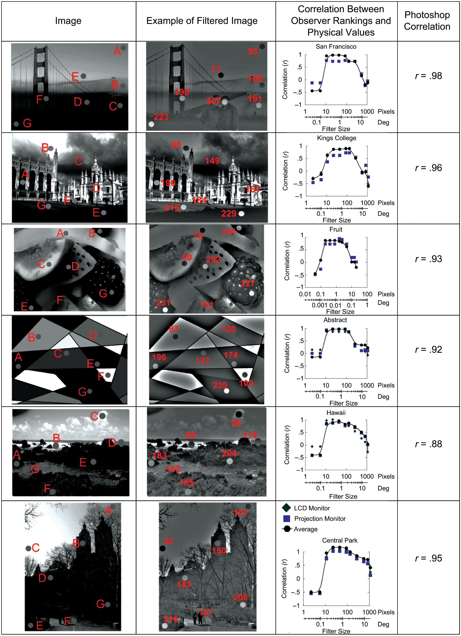
Experimental stimuli and results: the effect of removal of low-spatial-frequency content on the brightness of test disks placed at different locations on natural gray-scale images. The first column shows the original images (from top to bottom, titled San Francisco, Kings College, Fruit, Abstract, Hawaii, and Central Park); each image contained seven test disks (labeled “A” through “G”). All test disks had the same luminance level (i.e., the pixel value for each disk was 127), but the disks differed in apparent brightness. The second column shows the same six images after filtering according to Equation 1 (see the text); the test disks were no longer equiluminant. The red numbers in the filtered images indicate the average pixel value of each test disk (possible range: 0−255). The graphs plot the correlation between observers’ rankings of the brightness of the test disks in the unfiltered images and the rankings of the physical luminance values of these disks in the filtered images as a function of the size of the filter. The symbols in the plots show results for the two viewing conditions (LCD and projection monitor) and the correlations with the average rankings across all participants (the solid lines are smoothed fits to the average correlations); some of the symbols overlap because the results were similar in the two conditions. The fourth column shows the strength of the correlations between observers’ rankings and rankings of physical stimulus values when the images were filtered using Adobe Photoshop’s high-pass filter, with the filter radius equal to the size of the test disks. (The original images were obtained from the following people—San Francisco: Sara Wishner; Kings College: Scott Haefner, http://scotthaefner.com/; Fruit and Central Park: Penni Geller; Abstract and Hawaii: Claire Heidt.)

Note that the filtered disks in our stimuli (see Fig. 1, second column) were relatively homogeneous. A common complaint about lateral-inhibition models is that although test disks appear physically uniform, such models predict that they will have a scalloped (or inhomogeneous) profile (Gilchrist, 2006). In our procedure, a scalloped appearance occurs when the kernel width is smaller than the test disk, but not when the kernel is larger than the test disk. Larger kernels do not produce inhomogeneities in the test disks because these kernels average over regions larger than the disk area; consequently, the shading of the disks is not as sensitive to their spatial positioning.

Brightness Illusions in Natural Images

Does the perceived brightness of the test disks in the unfiltered images in Figure 1 correspond to the physical changes produced by high-pass filtering of the images? To answer this question, we had observers rank the brightness levels of the disks in the unfiltered images. We then averaged the rankings for each disk and calculated the correlation between these average rankings and the rankings of the pixel values of the test disks in the filtered images.

Application of the Filter to Hard-to-Explain Illusions

We also applied our high-pass filter (Equation 1) to stimuli that generate brightness illusions that are often considered to depend on contextual effects or to constitute evidence against simple lateral inhibition: Adelson’s (1995) checker-shadow illusion, an illusion in the style of Anderson and Winawer (2005), a texturized version of Adelson’s (2000) Argyle illusion, a simultaneous contrast illusion with an articulated surround (Gilchrist, 2006), and Bressan’s (2001) dungeon illusion (Fig. 2). In each case, the filtering process changed the physical luminance of the test patches, bringing their relative luminance in line with their relative perceived brightness before filtering. For instance, consider the checker-shadow illusion (Fig. 2, top row). In this illusion (column A), two squares that appear dark and bright, respectively, actually have identical luminance levels (which is apparent when a mask covers the rest of the checkerboard—see column B). These squares still appear physically different after application of our filter (column C), and in fact the test square that appears brighter in the unfiltered image has a physically higher luminance than the test square that appears darker in the unfiltered image (column D).

OPEN IN VIEWER

Fig. 2.

Removal of low-spatial-frequency content from stimuli that generate five brightness illusions. The filter from Equation 1 (see the text) was applied to Adelson’s (1995) checker-shadow illusion (top row), an illusion in the style of Anderson and Winawer (2005; second row), a texturized version of Adelson’s (2000) Argyle illusion (third row), a simultaneous contrast illusion with an articulated surround (Gilchrist, 2006; fourth row), and Bressan’s (2001) dungeon illusion (bottom row). In each case, the size of the averaging kernel was set to equal the diameter of the test patches. From left to right, the columns present the original images, the original images with a mask applied (to demonstrate that the test patches have the same luminance), the filtered images, and the filtered images with the mask applied (to show that the filtered test patches do not have the same luminance).

One particularly striking brightness illusion, Adelson’s (2000) snake/antisnake illusion (see Fig. 3), suggests that brightness perception depends on contextual inference. The test squares in the two rows of the snake display (Fig. 3, top right) have the same luminance but appear to be different from each other; the test squares in the two rows of the antisnake display (Fig. 3, bottom right) also have the same luminance, but they appear to be fairly similar to each other. This illusion is thought to be difficult to explain with filter models because the areas surrounding the test squares are identical in the two images, which differ physically only in the relative contrast of the half-ellipses that extend above and below the rectangular strips. The brightness of the test squares seems to depend on aspects of the display that are physically distant from the squares themselves (as Adelson, 2000, put it, “[it is as if] we can turn the contrast effect up or down by remote control” [p. 349]).

OPEN IN VIEWER

Fig. 3.

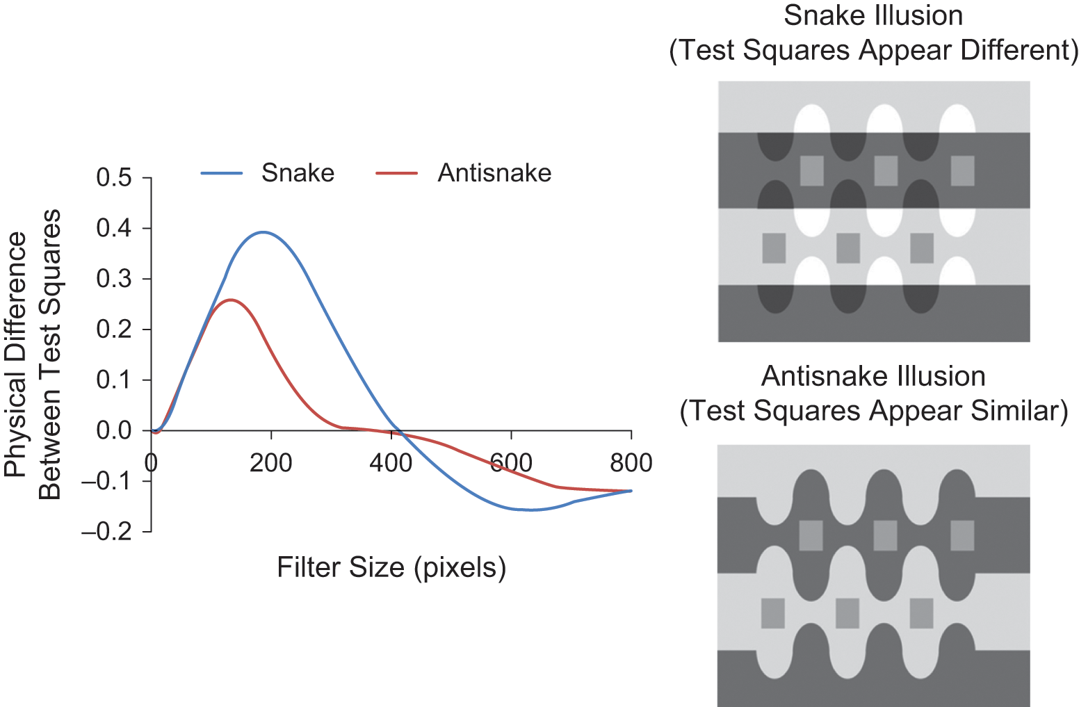
An examination of Adelson’s (2000) snake/antisnake illusion. Although the test squares in the snake display (upper right) all have the same luminance, the squares in the top row appear to be much brighter than those in the bottom row. The antisnake illusion (bottom right) is much weaker; in this case, again, the test squares in the display all have the same luminance, but their apparent brightness is fairly similar. The plot on the left shows the physical difference in relative luminance between the central squares in the two rows of each image when Equation 1 was applied (i.e., the low-spatial-frequency content was removed from the images). A value of 0 indicates that the two squares had the same average pixel value; a positive value indicates that the square in the top row had a higher physical value than the square in the bottom row. This difference in luminance of the test squares is shown as a function of the size of the kernel in Equation 1. Over a substantial range of filtering, the luminance difference was greater for the snake-illusion image than for the antisnake-illusion image.

However, the relative brightness of the test squares can also be accounted for in terms of the physical structure of the images. For each image, the graph in Figure 3 shows the difference between the luminance of the central test squares in the two rows when our high-pass filter (Equation 1) was applied; this difference was calculated by subtracting the average pixel value (range: 0−1) of the central test square in the bottom row from the average pixel value of the central test square in the top row. The graph plots this difference as a function of the diameter of the filter kernel in Equation 1. There was a substantial range of filtering for which the difference between the test squares was greater for the snake display than for the antisnake display. For instance, when the kernel size was between 200 and 300 pixels, the effect in the snake image was more than 6 times the effect in the antisnake image (the test squares were 220 pixels wide in the images used for analysis). The snake illusion was therefore physically stronger than the antisnake illusion at a spatial scale corresponding to the size of the test squares.

Discussion

Human visual cognition begins with early vision, which extracts physical properties from the visual scene (e.g., depth, brightness-color, texture, and surfaces); continues with midlevel vision, which extracts shape and spatial relations on the basis of outputs from early vision; and then culminates in high-level vision, which maps visual representations to meaning (Ullman, 1996). One critical question in vision science is how physical properties of the visual world are represented in early vision. We have posited a simple theory about early vision: Portions of the early human visual system act like an adaptive high-pass filter that removes low-spatial-frequency content from the visual world, with the cutoff frequency being determined by the image content. We have shown that a simple filtering process consistent with this hypothesis can account for relative differences in the brightness of equiluminant test patches in natural images, as well as for many hard-to-explain brightness illusions. In our examination of natural images, filtering was able to account for perceived brightness when the amount of blur discarded from the images corresponded to the size of the test discs, which suggests that the relevant scale for the low-spatial-frequency filtering performed by the visual system depends on the objects attended to in the visual scene.

The filtering process described here is a simple one- parameter model that effectively operates both as a method for discounting the illumination on an object and as a dynamic extension of lateral inhibition. Many Photoshop practitioners use Photoshop’s high-pass filter function to reduce the effects of shadows in images; yet although lateral inhibition acts like a high-pass filter, it is usually discussed in terms of edge extraction or accentuation of stationary contours (Ratliff, 1965), not in terms of the removal of blur or shadows (however, Ratliff did outline a process by which lateral inhibition could be extended to the elimination of motion blur). Sophisticated lateral-inhibition models that contain lateral inhibition in conjunction with a spatial weighting function (Shapley & Reid, 1985; Zaidi, Yoshimi, Flanigan, & Canova, 1992) would act more like a blur-removal process than an edge-extraction process and, as a result, would likely produce successful accounts for many of the illusions examined here. However, for such a model to account for changes in perception that arise when test patches are not fixed at midluminance, it is likely that the filter would need to be followed by a compressive nonlinear response function (e.g., Kingdom, 2003; Whittle, 1994).

Other investigators have successfully accounted for a wide range of brightness-lightness illusions with models that focus on spatial frequency (Blakeslee & McCourt, 1999; Blakeslee et al., 2005; Dakin & Bex, 2003; Perna & Morrone, 2007; Robinson et al., 2007). These models typically contain multiple banks of oriented spatial-frequency filters. Our approach differs because of the simplicity of our model—we reduced the filter banks to a single parameter—and because we examined the contextual effects in natural images. The additional parameters of other models may provide additional explanatory power, particularly in conditions in which contrast effects depend on orientation. The filter-based model most similar to ours is that of Perna and Morrone (2007), who proposed that most of these effects are contained primarily at a single spatial scale.

Models containing multiple filters have been criticized because they are structure blind; that is, “they have no provision for either acknowledging the crucial dependence of lightness on depth perception or distinguishing illuminance and reflectance edges” (Gilchrist, 2006, p. 212). Our model explicitly acknowledges a role for spatial organization by stating that filter size depends on the size of the most relevant stimulus. If elements in a scene are grouped to form a larger object, this would affect the scale of the high-pass filter. Indeed, the mere act of attending to an object has been shown to change the object’s perceived brightness (Tse, 2005); our approach could potentially account for this finding if attention causes selection of information at a relevant spatial scale.

A high-pass filter could also serve as the input to processes that compute absolute lightness of objects in a scene. For instance, anchoring theory proposes that the value of white is determined by the highest global luminance in the scene, and that the brightness of other objects depends on the relative weighting of potential Gestaltian frameworks (Gilchrist et al., 1999; Gilchrist & Radonjic, 2010). The model outlined in this article suggests that approaches like anchoring theory may be improved if object values are based on filtered responses, rather than on the measured luminance of the objects per se.

A number of brightness phenomena may at first seem difficult to explain with the one-parameter model. For instance, Equation 1 and a fixed kernel size cannot account for the following effects: (a) Articulated surrounds create stronger brightness effects than spatially uniform surrounds do (Gilchrist & Annan, 2002); (b) changes in the depth of a test patch relative to its surround can create marked changes in the perceived brightness or lightness of the test patch (Gilchrist, 1977); and (c) illusions of the type examined by Anderson and Winawer (2005) are remarkably strong when test patches are aligned with the background, but weak if the test patches are rotated 90°. Conceivably, such effects can be accounted for if the filter’s cutoff frequency changes as test patches become more or less separated from their backgrounds, or if the filter is capable of changing in response to additional parameters, such as orientation, articulation, and depth. However, it is also possible, and in some respects likely, that a one-parameter model cannot account for all of these effects. At the very least, one would expect that the filter would gradually weight low-spatial-frequency content (as opposed to having a sharp cutoff) and would be applied to local regions in the image instead of being applied uniformly across the entire image. Additionally, Equation 1, as it stands, cannot account for the long-range effects of brightness produced by Craik-O’Brian-Cornsweet (COB) edges. Intriguingly, Dakin and Bex’s (2003) finding that the perception of COB edges can be accounted for by boosting the visual response to low-spatial-frequency content suggests the possibility of processes that behave as if they reverse the sign of the subtraction in Equation 1.

Finally, one implication of our findings is that the counterintuitive aspects of most brightness illusions correspond to relative differences that are physically present in the images. That is, in a typical brightness illusion, the test patches are considered to be the same because they produce identical readings in a photometer that measures the light reflected from the patches. However, if the photometer contained a filter that removed the low-spatial-frequency content, then the photometer would record a different luminance level for each test patch, and the test patches would not be considered to be physically the same. The crucial factor for many brightness illusions may therefore reside in the physics of the stimuli, and human physiology may encode these physical properties by means of a neural process that is similar in principle to lateral inhibition.