The Effect of Relative Encoding on Memory-Based Judgments

Abstract

Several models of judgment propose that people struggle with absolute judgments and instead represent options on the basis of their relative standing. This leads to a conundrum when people make judgments from memory: They may encode an option’s ordinal rank relative to the surrounding options but later observe a different distribution of options. Do people update their representations when making judgments from memory, or do they maintain their representations based on the initial encoding? In three studies, we found that people making memory-based judgments rely on a stimulus’s relative standing in the distribution at the time of encoding rather than attending to absolute quality or updating the stimulus’s ordinal ranking in light of the distribution at the time of the later judgment.

Keywords

memory judgments ordinal rank encode open data open materials

People are bad at identifying or estimating the absolute magnitude of a stimulus, but are good at discriminating stimuli from one another (Garner, 1962; Laming, 1984, 1997; Miller, 1956; Shiffrin & Nosofsky, 1994; Stewart, Brown, & Chater, 2005; Stewart, Chater, & Brown, 2006). For example, it is very difficult for people to accurately identify the number of dots in a pattern, but they are better at determining which of two patterns contains more dots (e.g., Allik & Tuulmets, 1991; Kaufman, Lord, Reese, & Volkmann, 1949). Thus, some theories of decision making suggest that when assessing a stimulus, people represent where in a distribution that stimulus lies rather than the absolute value of that stimulus. These theories posit that people think about the value of stimuli on an ordinal scale (i.e., people determine that one stimulus is better than another but not by how much) or on an interval scale (i.e., people determine how much stimuli differ from one another in relative terms but not in relation to absolute standards; for a review, see Vlaev, Chater, Stewart, & Brown, 2011).

As a result, people’s evaluations of stimuli are heavily influenced by the surrounding context (e.g., Baird, Green, & Luce, 1980; Garner, 1954; Laming, 1997; Manis & Armstrong, 1971; Pepitone & DiNubile, 1976; Sherman, Ahlm, Berman, & Lynn, 1978; Simpson & Ostrom, 1976; Stewart & Brown, 2004; Stewart, Brown, & Chater, 2002). For example, circles are judged to be smaller when surrounded by large circles (the Ebbinghaus or Titchener circles illusion), sounds are judged as lower pitched when preceded by higher-pitched sounds (Campbell, Lewis, & Hunt, 1958), and moral transgressions are judged to be more severe when preceded by minor infractions (Parducci, 1968). In other words, there is a great deal of evidence that people’s judgments are regularly informed by relative rather than absolute standards.

A separate line of research has investigated how people make decisions when information about the choice options is not available at the time of choice (and thus needs to be drawn from memory). Specific information (e.g., the gas mileage or safety rating of a car) has been shown to be less accessible than overall evaluations (e.g., a holistic impression of the car’s favorability; Alba & Hutchinson, 1987; Chattopadhyay & Alba, 1988; Lingle, Geva, Ostrom, Leippe, & Baumgardner, 1979). As the use of overall evaluations and attribute information depends on the accessibility of these pieces of information (Lynch, Marmorstein, & Weigold, 1988), people often rely on memories of evaluations, rather than recalling the features of the options and then reevaluating the options at the time of choice (Carlston, 1980; Lichtenstein & Srull, 1985; Lingle et al., 1979; Lingle & Ostrom, 1979; Riskey, 1979).

This leads to an intriguing question. In the real world, people often are exposed to stimuli in one context (one distribution) and subsequently encounter new information about the nature of the distribution. If people’s judgments are relative rather than absolute, and if they recall their initial holistic impressions of stimuli when evaluating those stimuli from memory, then people may evaluate options in relation to the context in which they first learned about the options, rather than the updated context in which they are making the choice. To what extent does the evaluation of a stimulus change after people accrue new information about the distribution from which it was drawn?

For example, to a college student who eats primarily dormitory food, a meal at the local pub might be in the 99th percentile in the quality of his dining experiences, and he would encode it in memory as such. After he leaves college and samples non–dorm food (most of which is better than what was available at the dorm), that pub meal might fall at the 50th percentile of his (now expanded) distribution of food quality. If a friend asks him about the quality of the food at the pub, will he recall it as a 99th-percentile meal (as he initially encoded it), or will he have updated his representation of the meal to take into account that the distribution of his dining experiences has changed since the time of initial encoding?

In this article, we report three studies in which we demonstrated that people naturally encode a stimulus in reference to its relative position in its comparison class at the time of initial exposure and fail to update their representation in the context of a new distribution.

Study 1: Judgments of Quality

Method

In Study 1, participants listened to several song clips (ostensibly from a singing competition) drawn from one distribution of quality. After a delay, they were exposed to additional clips. Participants were then asked to evaluate all of the songs from the expanded distribution. The key question was whether participants would make judgments that aligned with a song’s relative position in the original set at Time 1 or if their judgments would align with the song’s relative position in the expanded distribution.

Stimuli

A series of clips of singers was downloaded from YouTube. Audio-only files of the clips were pretested on Amazon Mechanical Turk by 71 participants. Ten to 11 participants evaluated each clip by rating how good they thought the singer was on a 7-point Likert scale (1 = not good at all, 7 = very good). We selected two clips that were perceived to be very bad (M = 1.50, SD = 0.85; M = 1.70, SD = 0.95), three clips that were perceived to be average (M = 3.90, SD = 0.87; M = 3.90, SD = 1.00; M = 3.70, SD = 1.16), and two clips that were perceived to be very good (M = 6.20, SD = 0.63; M = 6.00, SD = 1.16).

Participants

One hundred paid Amazon Mechanical Turk workers (60 men and 40 women; age range: 19–63 years, M = 33.80) completed the study.¹

Procedure

Participants were asked to imagine that they were judges at a singing competition and would listen to competitors in two auditions, the first in Los Angeles and the second in New York City. They were randomly assigned to one of two conditions. Half of the participants first listened to the two very bad singers and then to one average singer (the target singer). Because the target singer was at the top of the Time 1 distribution, we refer to this condition as the T1-top condition. The other half of the participants first listened to the two very good singers and then to one average singer (the target singer). Because the target singer was at the bottom of the Time 1 distribution, we refer to this condition as the T1-bottom condition.

After listening to the three clips, participants were told to imagine that they were traveling to the next audition and needed to tune their recording equipment. They then engaged in a distractor task designed to clear auditory memory. On each trial, they listened to a series of four sounds sequentially and were then asked a question about the sounds. They completed five trials, with a different question asked on each trial (e.g., which sound played the longest, which sound had the lowest pitch).

After this distractor task, participants were told that they had arrived in New York City. All of the participants, regardless of condition, then listened to two average, nontarget, singers (roughly equal in quality to the target singer according to the pretest). Which average singer was the target singer and which average singers were the nontarget singers were counterbalanced across participants.

At the end of the second set of auditions, participants chose one singer as the winner of the competition. They also selected one contestant to eliminate, in a procedure akin to the approach on American Idol (Blankens, 2002–2016).

Results

The overall quality of the set of singers that participants were exposed to was better in the T1-bottom condition than in the T1-top condition. In both conditions, there were three average singers; however, in the T1-top condition, the rest of the distribution was poor quality, and in the T1-bottom condition, the rest of the distribution was good quality. We found that the participants were sensitive to the quality of the comparison set. They were significantly more likely to choose the target singer as the winner when the distribution included two bad singers (the T1-top condition; 40.8%) than when the distribution included two good singers (the T1-bottom condition; 2.0%), χ²(2, N = 100) = 22.74, p < .001, r = .477, and significantly less likely to choose the target singer to be eliminated in the T1-top condition (6.1%) than in the T1-bottom condition (37.3%), χ²(2, N = 100) = 14.11, p < .001, r = .376. However, 10 participants chose one of the bad singers as the winner or eliminated one of the good singers and were excluded from the following analysis.²

When making decisions after having been exposed to an expanded distribution, participants still appeared to rely on the initial evaluation of the target singer. Compared with what one would expect by chance, when participants in the T1-top condition chose an average-quality singer as the winner and when participants in the T1-bottom condition chose an average-quality singer as the singer to be eliminated, they were significantly more likely to choose the target singer than to choose one of the other average-quality singers (43% chose the target singer, chance = 33.33%), χ²(2, N = 90) = 4.05, p = .044, r = .212. (See Fig. 1 for the percentage of participants in each condition who chose the target singer as the winner and who chose the target singer as the singer to be eliminated and the average percentage of participants in each condition who chose a nontarget singer as the winner and who chose a nontarget singer as the singer to be eliminated.)

Fig. 1.

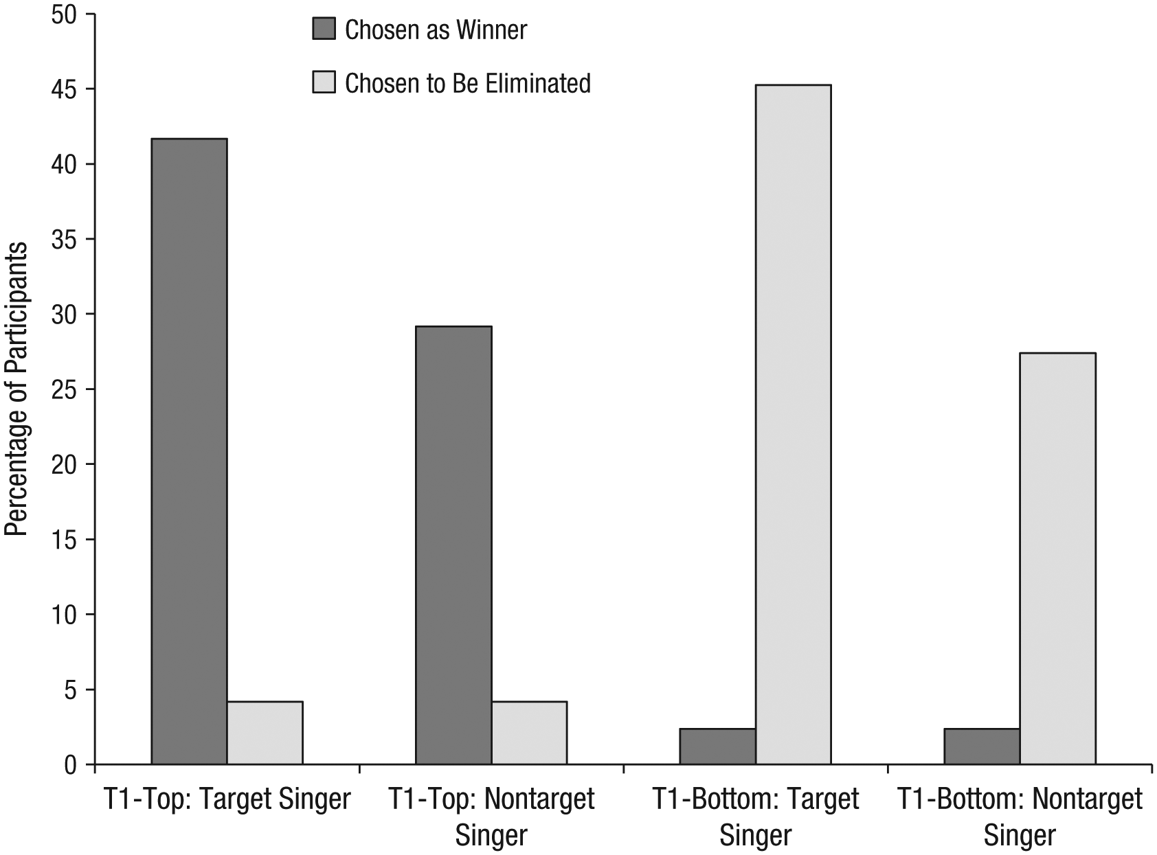
Results from Study 1: percentage of participants who chose the target singer as the winner and who chose the target singer as the singer to be eliminated and average percentage of participants who chose a nontarget average singer as the winner and who chose a nontarget average singer as the singer to be eliminated. Percentages were calculated separately for participants in the Time 1 (T1)-top and T1-bottom conditions.

Discussion

Replicating dozens of prior studies, Study 1 demonstrated that participants’ evaluations are made relative to the comparison set at the time of evaluation (Time 1). Additionally, this study showed that an evaluation initially encoded at Time 1 is used in memory-based choices at a subsequent time. Evaluations from Time 1 were not adequately updated to reflect changes in the distribution that occurred after the evaluations were encoded into memory. Within each condition (i.e., the T1-top or the T1-bottom condition), although participants had been exposed to the same distribution of singers (i.e., they had listened to the same five singers) at the time of judgment, they made different choices about the same average singer depending on whether they initially encoded that singer in the context of a smaller distribution, at Time 1, or as part of a larger distribution, at Time 2. In Study 2, we aimed to determine whether this effect would generalize to a different type of judgment.

Study 2: Judgments of Speed

Method

It can be argued that judgments of quality are inherently subjective because there are no absolute criteria for assessing or encoding quality. Thus, it is plausible that the patterns of results we observed in Study 1 would be found only for domains in which relative (as opposed to absolute) judgments are obligatory. The purpose of Study 2 was to determine whether our findings would generalize to a domain in which there exist objective truths and it is possible to make absolute judgments. Therefore, in Study 2, we asked participants to watch toy cars race and judge the speed of the cars.

Participants

One hundred twenty-one participants from a large university in the Southwest United States completed this study.³

Procedure

Participants came into the lab and were informed that they would be asked to evaluate the speed of pull-back toy cars. They were told that they would watch two cars race in Phase 1 of the study and then watch another car race along the same track in Phase 2 of the study. The research assistant explained that they should try to remember the speeds of the cars during Phase 1 so that they could later rank all of the cars.

In each lab session, a group of 3 to 6 participants was randomly assigned to the T1-bottom condition or the T1-top condition. In Phase 1, participants in the T1-bottom condition watched a research assistant race a fast yellow car and a moderate-speed black car (the target car). Participants in the T1-top condition watched a research assistant race a slow red car and a moderate-speed black car (the target car; the same car used in the T1-bottom condition). The cars moved along the track simultaneously, so participants could observe the contrast in the speeds of the cars. The orange track was in the middle of the lab, and participants sat in chairs to the right and left of the track. An object was placed approximately 5 ft away from the start of the track to stop the cars. Therefore, the cars stopped at the same point on the track regardless of the speed at which they were going (but the faster car reached that point more quickly).

Participants then engaged in a filler task for 5 to 10 min.⁴ After the filler task, they came back to the track. They were told that the research assistant would now race a different black car along the track. In reality, however, this was the same black car that was used in Phase 1, and it moved at the same speed as in Phase 1. We refer to this car as the decoy car.

Finally, participants were asked to rank all “three” cars according to their speed (1 = fastest, 3 = slowest).

Results

Thirteen participants’ responses were excluded from analysis because a car malfunctioned. Additionally, 1 participant chose the red car as the fastest car, thus failing the manipulation check, and was eliminated from analysis.

As in Study 1, the overall distribution that participants were exposed to differed between the T1-top condition and the T1-bottom condition. In the T1-bottom condition, the target car had an actual rank of 2.5 (both the target car and the decoy car were slower than the fast yellow car). In the T1-top condition, the target car had an actual rank of 1.5 (both the target car and the decoy car were faster than the slow red car).

For each participant, we computed a deviation score that represented how far the participant’s ranking of the target car deviated from its actual rank (T1-top condition: deviation score = participant’s ranking – 1.5; T1-bottom condition: deviation score = participant’s ranking – 2.5). We found that participants’ speed judgments were influenced by the context in which they viewed the cars. The mean deviation scores in the T1-top condition (M = −0.367) and the T1-bottom condition (M = 0.065) differed significantly, t(105) = 4.56, p < .001, 95% confidence interval (CI) for the difference = [0.2438, 0.6185], d = 0.93.

The deviation scores also showed that participants failed to update their representations of the target car after seeing an expanded distribution. Participants in the T1-bottom condition ranked the target car as slower than it actually was, and participants in the T1-top condition ranked the target car as faster than it actually was. Further, participants were significantly more likely than expected by chance to rank the target car, rather than the decoy car, as the fastest car in the T1-top condition and as the slowest car in the T1-bottom condition (72% chose the target car, chance = 50%), χ²(2, N = 106) = 19.96, p < .001, r = .434. (See Fig. 2 for the percentage of participants in each condition who ranked the target car and the decoy car as the fastest car and as the slowest car.)

Fig. 2.

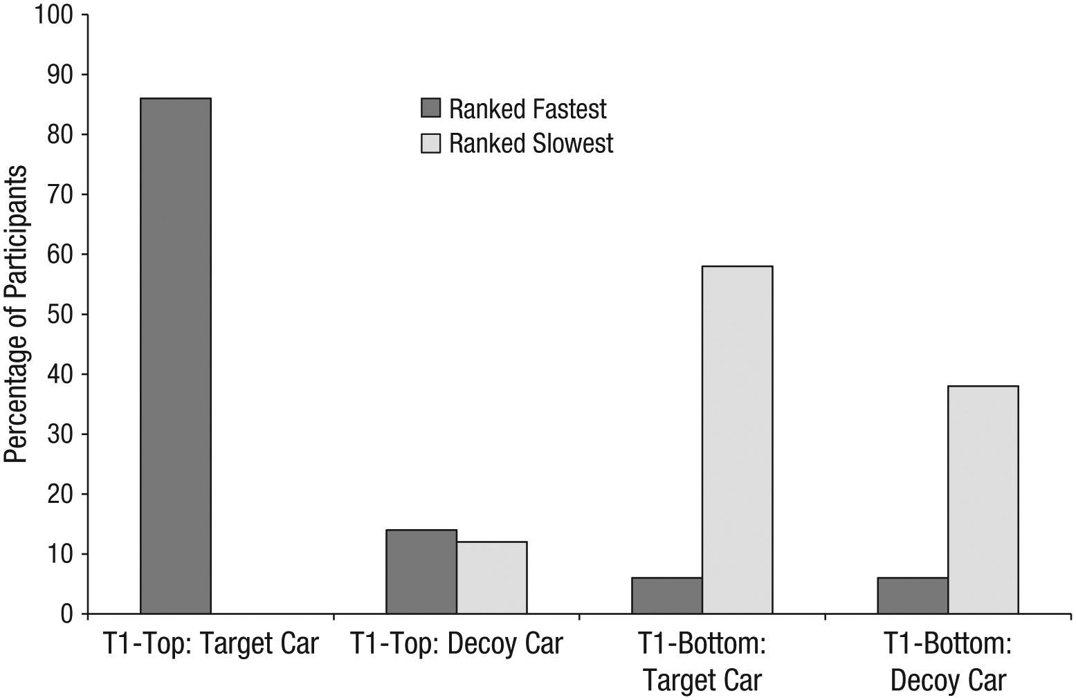
Results from Study 2: percentage of participants who ranked the target car and the decoy car as the fastest car and as the slowest car, separately for participants in the Time 1 (T1)-top and T1-bottom conditions.

Discussion

This study replicated the results from Study 1 with a different dependent measure—speed judgments—for which there was an objectively correct answer. Participants appeared to evaluate the speeds of the cars on the basis of how they compared at Time 1, and when the distribution of cars expanded, participants failed to update their initial impressions.

However, in both Studies 1 and 2, participants were asked to make relative, ordinal judgments (i.e., choose the winner and loser in Study 1 and rank the cars in Study 2), which could have biased them toward this type of comparative reasoning. To what extent would the observed effect hold when the judgment of interest is absolute (e.g., the quantity of a stimulus) rather than relative? To answer this question, in Study 3, we manipulated the dependent variable, such that half of the participants made absolute judgments of quantity and half made inherently comparative judgments of quantity (rank order).

Additionally, Study 3 examined a situation in which participants encoded the stimuli dynamically over time and the distributions were larger. Another change from Studies 1 and 2 was that the dependent variable was a prediction for the future rather than an estimation concerning the past.

Study 3: Judgments of Quantity

Method

Participants

Four hundred paid Amazon Mechanical Turk participants (198 males and 202 females; age range: 18–72 years, M = 36.27) completed this study.⁵

Procedure

Participants were told to imagine that they were an intern for a team of lepidopterists and that they were assigned to observe the butterflies that landed on eight different flowers. Because of limited funding, they would be able to observe only four flowers each week, so they would watch four of the flowers in the first week and the other four flowers in the second week. They were asked to observe each group of four flowers for 7 days. Each day, they could observe the flowers for only 4 s because the butterflies would fly away if they noticed an observer watching. After the 2 weeks were over, the lepidopterists would ask participants questions about the flowers. (Note that “days” and “weeks” in this study refer to time in the fictional scenario. Participants completed the entire scenario in one sitting over the course of 10 to 15 min.)

The flowers were depicted as seven-point stars, and the butterflies on the flowers were small images of an orange butterfly. To the right of each star, there was a picture of a real flower along with the name of the flower. Before beginning each week of observations, participants familiarized themselves with the names and pictures of the flowers, so they would be able to identify them more easily later.

After familiarizing themselves with the four flowers for Week 1, for each of the 7 days, participants observed those flowers, one of which was the target flower. The number of butterflies on the flowers changed subtly from day to day (with a maximum change of 3 butterflies per flower on any given day). Because of the changing number of butterflies and their changing positions on the flowers from day to day, the butterflies appeared to move between flowers across days; thus, the stimuli represented the stochastic nature of the system. The target flower had an average of 40 butterflies on it. Participants were randomly assigned to the T1-top condition, in which the three other flowers had fewer butterflies than the target flower (an average of approximately 25 butterflies per flower), or the T1-bottom condition, in which the same three other flowers had more butterflies than the target flower (an average of approximately 60 butterflies per flower). Participants saw the same set of four flowers for 4 s each day.

Afterward, participants were told that the lepidopterists wanted to test their visual working memory before the next week of observations. On each trial of this distractor task, participants were shown a series of five objects that differed in shape, color, and size and were asked a question about them (e.g., which shape was the biggest). A different question was asked on each of four trials. This task was designed to clear visual working memory.

In Week 2, participants observed a different set of four flowers. Two of these flowers—the moderate-low and extreme-low flowers—had on average fewer butterflies than the target flower (approximately 37 and 34 butterflies, respectively). The other two flowers—the moderate-high and extreme-high flowers—had on average more butterflies than the target flower (approximately 43 and 48 butterflies, respectively). The number of butterflies on these flowers also changed subtly from day to day (with a maximum change of 3 butterflies per flower on any given day). Aside from the differences in the flowers and numbers of butterflies, the procedure for Week 2 was identical to the procedure from Week 1.

Next, participants were randomly assigned to either the relative-judgment or the absolute-judgment condition. Participants in both conditions were asked the same question: “Based on your observations, how many butterflies do you think will be on each of the flowers next month?” However, the manner in which participants answered this question differed between the conditions. In the absolute-judgment condition, participants were asked to predict the number of butterflies on each flower. In the relative-judgment condition, participants were asked to rank all eight flowers according to their expected butterfly population.

Results

As participants in the two conditions responded to the judgment question on different types of scales (rank order vs. estimation), the relative-judgment and absolute-judgment conditions were analyzed separately.

Absolute judgments

Three outliers more than 4 standard deviations from the mean were removed from analysis. One individual wrote qualitative text responses rather than numerical responses and thus also could not be included in the analysis. Responses were not normally distributed and were therefore natural-log transformed for all inferential statistics. However, we report raw numbers to provide readers with an intuitive sense of the effects (for a graphical display of the actual numbers of butterflies and participants’ mean predictions, see Fig. 3).

Fig. 3.

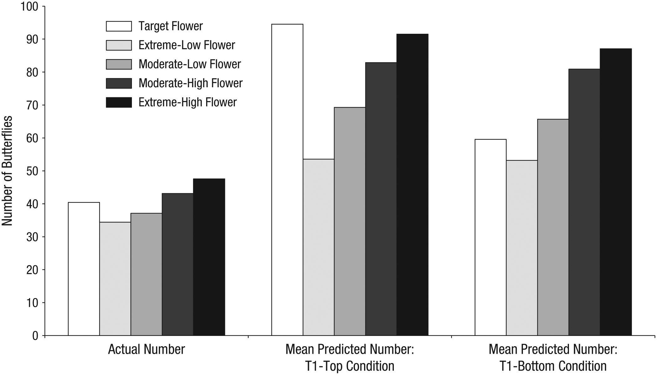
Results from Study 3: mean predicted number of butterflies on the target, extreme-low, moderate-low, moderate-high, and extreme-high flowers, separately for the Time 1 (T1)-top condition and the T1-bottom condition. Also graphed are the actual mean numbers of butterflies that had been shown on those flowers.

Participants predicted that there would be significantly more butterflies on the target flower in the T1-top condition (M = 94.54) than in the T1-bottom condition (M = 59.57), t(189) = 2.46, p = .015, 95% CI for the natural-log difference = [0.07774, 0.70215], d = 0.36. This suggests that participants were sensitive to the context in which they encoded the target flower.

Two of the Week 2 flowers (the extreme-low and moderate-low flowers) actually had fewer butterflies than the target flower. For this reason, it is not surprising that participants in the T1-top condition accurately⁶ estimated that the target flower would have more butterflies than these two flowers (target: M = 94.54; extreme-low: M = 53.56; moderate-low: M = 69.28), t(94) = 11.97, p < .001, 95% CI for the natural-log difference = [0.39802, 0.55627], d = 1.27, and t(94) = 6.69, p < .001, 95% CI for the natural-log difference = [0.17872, 0.32958], d = 0.70, respectively. However, two of the Week 2 flowers (the moderate-high and extreme-high flowers) actually had more butterflies than the target flower. Participants also estimated that the target flower would have significantly more butterflies than the moderate-high flower (M = 82.86), t(94) = 2.20, p = .030, 95% CI for the natural-log difference = [0.00780, 0.15072], d = 0.23, and nonsignificantly more butterflies than the extreme-high flower (M = 91.52), t(94) = 1.40, p = .166, 95% CI for the natural-log difference = [−0.02397, 0.13472].

Although the number of butterflies on the target flower was the same in the T1-bottom condition as in the T1-top condition, the pattern of results was qualitatively different. In the T1-bottom condition, participants accurately estimated that the target flower would have fewer butterflies than the extreme-high and moderate-high flowers, which actually had more butterflies (target: M = 59.57; extreme-high: M = 87.09; moderate-high: M = 80.90), t(95) = −8.41, p < .001, 95% CI for the natural-log difference = [−0.44228, −0.27338], d = 0.87, and t(95) = −8.71, p < .001, 95% CI for the natural-log difference = [−0.41231, −0.25924], d = 0.89, respectively. However, participants also estimated that the target flower would have fewer butterflies than the moderate-low flower (M = 65.68), t(95) = −3.21, p = .002, 95% CI for the natural-log difference = [−0.22206, −0.05225], d = 0.33, and there was no significant difference in the predicted number of butterflies on the target flower and the extreme-low flower (M = 53.18), t(95) = 1.42, p = .158, 95% CI for the natural-log difference = [−0.02026, 0.12290]. In other words, relative to their predictions for the nontarget flowers, participants overestimated the number of butterflies on the target flower in the T1-top condition but underestimated the number of butterflies on the target flower in the T1-bottom condition.

Relative judgments

In the relative-judgment condition, a score of 1 was given to the flower ranked to have the fewest butterflies and a score of 8 was given to the flower ranked to have the most butterflies. Across the two distribution conditions, five of the flowers were the same (the target flower at Week 1 and the four flowers at Week 2). However, the three flowers shown with the target flower at Week 1 differed between the T1-top and T1-bottom condition. As a result, the target flower had a different actual rank depending on condition: an actual rank of 6 (out of 8) in the T1-top condition and an actual rank of 3 (out of 8) in the T1-bottom condition (for a graphical display of the actual and predicted ranks of the flowers common to the T1-top and T1-bottom conditions, see Fig. 4).

Fig. 4.

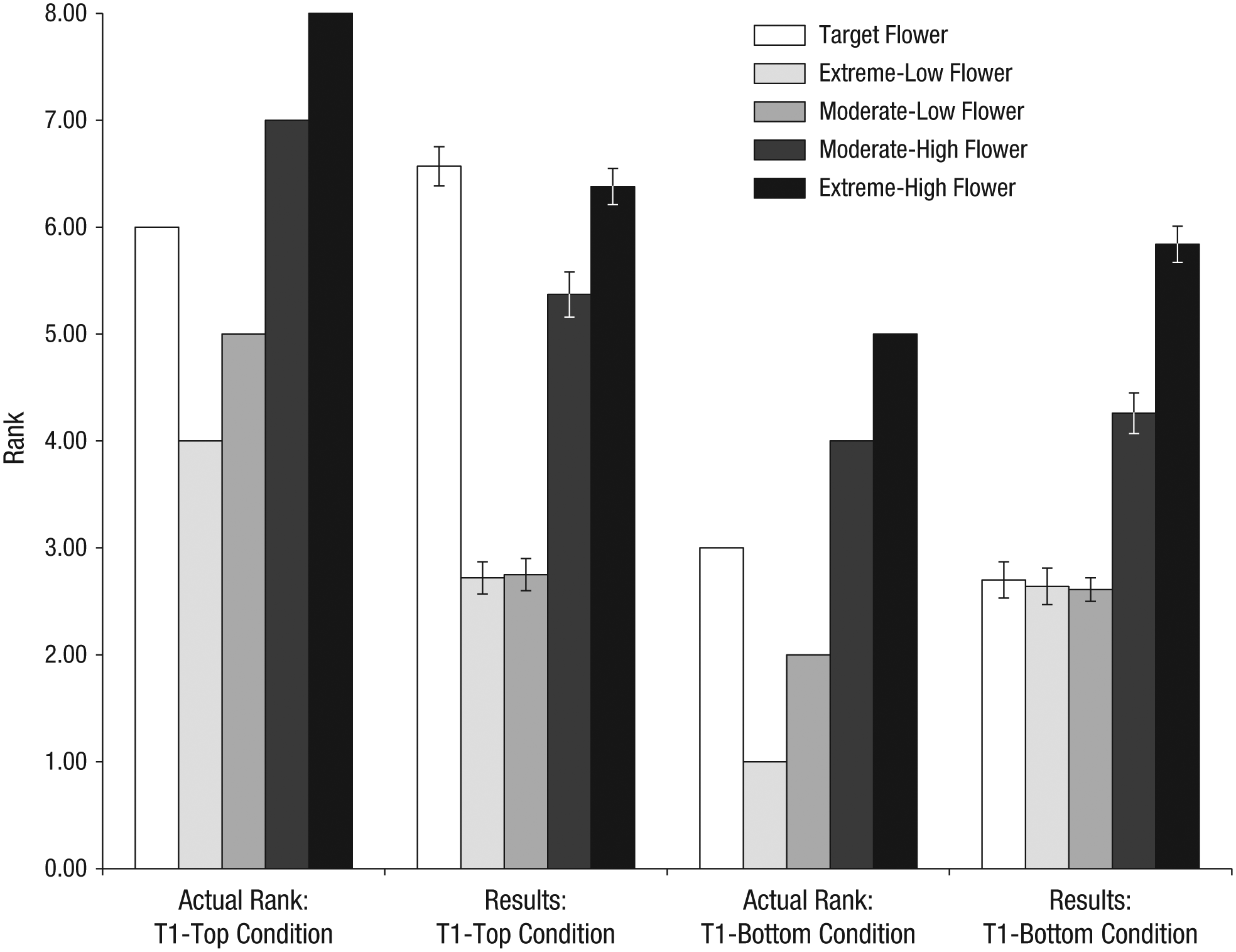
Results from Study 3: participants’ average ranking of the target, extreme-low, moderate-low, moderate-high, and extreme-high flowers, separately for the Time 1 (T1)-top condition and the T1-bottom condition. Also graphed are the flowers’ actual rankings in each condition. Error bars represent ±1 SE.

For this reason, in order to analyze the data, we computed a deviation score that represented how far a participant’s ranking of the target flower deviated from its actual ranking (T1-top condition: deviation score = participant’s ranking – 6; T1-bottom condition: deviation score = participant’s ranking – 3). The T1-top and T1-bottom deviation scores were significantly different from each other (T1-top: M = 0.57; T1-bottom: M = −0.30), t(203) = −3.47, p = .001, 95% CI for the difference = [−1.363, −0.376], d = 0.48. In the T1-top condition, participants ranked the target flower significantly higher than its actual rank (6.6 vs. 6.0), t(101) = 3.10, p = .003, 95% CI for the difference = [0.2045, 0.9327]. However, in the T1-bottom condition, participants ranked the target flower marginally significantly lower than its actual rank (2.7 vs. 3.0), t(102) = −1.764, p = .081, 95% CI for the difference = [−.6393, .0374]. This analysis revealed that, as in the absolute-judgment condition, participants overestimated the number of butterflies in the T1-top condition and underestimated the number of butterflies in the T1-bottom condition (for additional analyses, see Appendix S1 in the Supplemental Material available online).

Discussion

Study 3 replicated the findings from Studies 1 and 2. Participants relied on their memory of where the target stimulus stood in the distribution at Time 1 even when making judgments after exposure to an expanded distribution. This study showed that the effect generalized beyond relative judgments to judgments of absolute quantity. Further, it demonstrated that the effect holds in a dynamic setting, over multiple observations of the stimuli.

General Discussion

Prior research has suggested that people encode information relative to the context. Further research has shown that when making judgments from memory, people tend to rely on their initial, holistic impressions (which were influenced by that initial context). The present research builds on these prior findings, showing that people rely on their initial evaluation even when the context at Time 2 has changed. In three experiments, people encoded information relative to the context (or distribution) at Time 1 and failed to update this representation in a new distribution when making judgments.

Expertise in the relevant judgment domain may moderate this effect. Lynch, Chakravarti, and Mitra (1991) found that contrast effects (i.e., inverse relations between ratings of a stimulus and the values of the context stimuli) arose for different reasons among participants with high knowledge about the stimuli and those with low knowledge about the stimuli. Contrast effects arose because of a change in the mental representations of target stimuli (i.e., how people actually thought about the objects they rated) only among people who had low knowledge about the stimuli. Among those who had high knowledge about the stimuli, contrast effects were due to scale anchoring (i.e., how participants labeled the categories of the researchers’ scales); thus, experts do not change how they actually think about a stimulus on the basis of the context stimuli. In our studies, we used nonexpert samples (undergraduates and Mechanical Turk participants). Therefore, the effects we observed were likely due to participants mentally representing and encoding the target stimuli at Time 1 differently, on the basis of the surrounding options (i.e., T1-top or T1-bottom condition), and then failing to update those representations in the new context at Time 2. However, because experts do not use context stimuli as the basis for how they actually think about a target stimulus, the local context at Time 1 may not affect their representations of target stimuli, and therefore their subsequent judgments of those stimuli may be more accurate. Future research should test if the effect reported here is moderated by expertise.

Our results suggest that in making memory-based judgments, people should be cautious of how the original context in which the stimuli were encoded may bias later estimates. Judgments are often at least partially based on memory. By exploring how memory distortions may affect judgments, researchers can better understand how and why people make biased judgments and choices.

Footnotes

Action Editor

Hal Arkes served as action editor for this article.

Declaration of Conflicting Interests

The authors declared that they had no conflicts of interest with respect to their authorship or the publication of this article.

Supplemental Material

Additional supporting information can be found at

Open Practices

All data and materials have been made publicly available via Open Science Framework and can be accessed at https://osf.io/r5kcn/. The complete Open Practices Disclosure for this article can be found at http://pss.sagepub.com/content/by/supplemental-data. This article has received badges for Open Data and Open Materials. More information about the Open Practices badges can be found at https://osf.io/tvyxz/wiki/1.%20View%20the%20Badges/and .

Notes

References

Alba

J. W.

Hutchinson

J. W.

(1987). Dimensions of consumer expertise. Journal of Consumer Research, 13, 411–454.

Allik

Tuulmets

(1991). Occupancy model of perceived numerosity. Perception & Psychophysics, 49, 303–314.

Baird

J. C.

Green

D. M.

Luce

R. D.

(1980). Variability and sequential effects in cross-modality matching of area and loudness. Journal of Experimental Psychology: Human Perception and Performance, 6, 277–289.

Blankens

(Producer). (2002–2016). American idol [Television series]. Los Angeles, CA: Fox Studios.

Campbell

D. T.

Lewis

N. A.

Hunt

W. A.

(1958). Context effects with judgmental language that is absolute, extensive, and extra-experimentally anchored. Journal of Experimental Psychology, 55, 220–228.

Carlston

D. E.

(1980). The recall and use of traits and events in social inference processes. Journal of Experimental Social Psychology, 16, 303–328.

Chattopadhyay

Alba

J. W.

(1988). The situational importance of recall and inference in consumer decision making. Journal of Consumer Research, 15, 1–12.

Garner

W. R.

(1954). Context effects and the validity of loudness scales. Journal of Experimental Psychology, 48, 218–224.

Garner

W. R.

(1962). Uncertainty and structure as psychological concepts. New York, NY: Wiley.

10.

Kaufman

E. L.

Lord

M. W.

Reese

T. W.

Volkmann

(1949). The discrimination of visual number. The American Journal of Psychology, 62, 498–525.

11.

Laming

(1984). The relativity of ‘absolute’ judgements. British Journal of Mathematical and Statistical Psychology, 37, 152–183.

12.

Laming

(1997). The measurement of sensation. Oxford, England: Oxford University Press.

13.

Lichtenstein

Srull

T. K.

(1985). Conceptual and methodological issues in examining the relationship between consumer memory and judgment. In Alwight

L. F.

Mitchell

A. A.

(Eds.), Psychological processes and advertising effects (pp. 113–128). Hillsdale, NJ: Erlbaum.

14.

Lingle

J. H.

Geva

Ostrom

T. M.

Leippe

M. R.

Baumgardner

M. H.

(1979). Thematic effects of person judgments on impression organization. Journal of Personality and Social Psychology, 37, 674–687.

15.

Lingle

J. H.

Ostrom

T. M.

(1979). Retrieval selectivity in memory-based impression judgments. Journal of Personality and Social Psychology, 37, 180–194.

16.

Lynch

J. G.

Jr. Chakravarti

Mitra

(1991). Contrast effects in consumer judgments: Changes in mental representations or in the anchoring of rating scales? Journal of Consumer Research, 18, 284–297.

17.

Lynch

J. G.

Jr. Marmorstein

Weigold

M. F.

(1988). Choices from sets including remembered brands: Use of recalled attributes and prior overall evaluations. Journal of Consumer Research, 15, 169–184.

18.

Manis

Armstrong

G. W.

(1971). Contrast effects in verbal output. Journal of Experimental Social Psychology, 7, 381–388.

19.

Miller

G. A.

(1956). The magical number seven, plus or minus two: Some limits on our capacity for processing information. Psychological Review, 63, 81–97.

20.

Parducci

(1968). The relativism of absolute judgments. Scientific American, 219, 84–90.

21.

Pepitone

DiNubile

(1976). Contrast effects in judgments of crime severity and the punishment of criminal violators. Journal of Personality and Social Psychology, 33, 448–459.

22.

Riskey

D. R.

(1979). Verbal memory processes in impression formation. Journal of Experimental Psychology: Human Learning and Memory, 5, 271–281.

23.

Sherman

S. J.

Ahlm

Berman

Lynn

(1978). Contrast effects and their relationship to subsequent behavior. Journal of Experimental Social Psychology, 14, 340–350.

24.

Shiffrin

R. M.

Nosofsky

R. M.

(1994). Seven plus or minus two: A commentary on capacity limitations. Psychological Review, 10, 357–361.

25.

Simpson

D. D.

Ostrom

T. M.

(1976). Contrast effects in impression formation. Journal of Personality and Social Psychology, 34, 625–629.

26.

Stewart

Brown

G. D.

(2004). Sequence effects in the categorization of tones varying in frequency. Journal of Experimental Psychology: Learning, Memory, and Cognition, 30, 416–430.

27.

Stewart

Brown

G. D.

Chater

(2002). Sequence effects in categorization of simple perceptual stimuli. Journal of Experimental Psychology: Learning, Memory, and Cognition, 28, 3–11.

28.

Stewart

Brown

G. D.

Chater

(2005). Absolute identification by relative judgment. Psychological Review, 112, 881–911.

29.

Stewart

Chater

Brown

G. D.

(2006). Decision by sampling. Cognitive Psychology, 53, 1–26.

30.

Vlaev

Chater

Stewart

Brown

G. D.

(2011). Does the brain calculate value? Trends in Cognitive Sciences, 15, 546–554.

Supplementary Material

Please find the following supplemental material available below.

For Open Access articles published under a Creative Commons License, all supplemental material carries the same license as the article it is associated with.

For non-Open Access articles published, all supplemental material carries a non-exclusive license, and permission requests for re-use of supplemental material or any part of supplemental material shall be sent directly to the copyright owner as specified in the copyright notice associated with the article.

0.00 MB

0.58 MB

0.22 MB