Gaze Amplifies Value in Decision Making

Abstract

When making decisions, people tend to choose the option they have looked at more. An unanswered question is how attention influences the choice process: whether it amplifies the subjective value of the looked-at option or instead adds a constant, value-independent bias. To address this, we examined choice data from six eye-tracking studies (Ns = 39, 44, 44, 36, 20, and 45, respectively) to characterize the interaction between value and gaze in the choice process. We found that the summed values of the options influenced response times in every data set and the gaze-choice correlation in most data sets, in line with an amplifying role of attention in the choice process. Our results suggest that this amplifying effect is more pronounced in tasks using large sets of familiar stimuli, compared with tasks using small sets of learned stimuli.

Keywords

decision making computational modeling eye tracking attention drift-diffusion model

Many of the decisions that we make on a daily basis (e.g., choices between foods, consumer goods, and even complex moral dilemmas) are shaped by attention. The decision process is often modeled as an evidence-accumulation process, through which the potential options compete for the participant’s choice. Visual attention is known to affect this evidence-accumulation process. Past research (Armel, Beaumel, & Rangel, 2008; Cavanagh, Wiecki, Kochar, & Frank, 2014; Fiedler & Glöckner, 2012; Fiedler, Glöckner, Nicklisch, & Dickert, 2013; Folke, Jacobsen, Fleming, & De Martino, 2016; Krajbich, Armel, & Rangel, 2010; Krajbich, Lu, Camerer, & Rangel, 2012; Krajbich & Rangel, 2011; Lim, O’Doherty, & Rangel, 2011; Mormann, Navalpakkam, Koch, & Rangel, 2012; Pärnamets et al., 2015; Stewart, Hermens, & Matthews, 2016; Towal, Mormann, & Koch, 2013) has shown that gaze to an alternative increases the likelihood of choosing that option, even after one accounts for the subjective values of the alternatives. These studies come from a variety of domains, suggesting that many decisions are influenced by attention.

Thus far, sequential-sampling models (SSMs) have been successfully used to characterize the attention-influenced decision process (Ashby, Jekel, Dickert, & Glöckner, 2016; Busemeyer & Diederich, 2002; Busemeyer & Townsend, 1993; Fisher, 2017; Krajbich et al., 2010; Krajbich et al., 2012; Krajbich & Rangel, 2011; Krajbich & Smith, 2015; Towal et al., 2013; Vaidya & Fellows, 2015). The general idea behind these models is that over time, evidence is noisily accumulated for each of the options; once enough evidence is accumulated for one option—relative to the other—the decision is made. However, the precise mechanism that underlies the effect of attention on the evidence-accumulation process has not been established. A couple different SSMs rooted in the drift-diffusion model (DDM; Ratcliff, 1978) have been proposed thus far, and both are capable of capturing several trends in choice and eye-tracking data.

The main thing that differentiates these models is the interaction of value and attention. One model proposes that attention gives a fixed, additive boost to the evidence accumulated for the gazed-at option (Cavanagh et al., 2014). This additive model posits that gaze is indicative of the decision maker’s instantaneous bias toward an option, the magnitude of which is independent of the option itself. Another model, the attentional DDM (aDDM; Krajbich et al., 2010), suggests an interaction between the values of the options and the degree to which attention influences the evidence-accumulation process. In this sense, attention to an option amplifies its representation in the mind of the decision maker. Thus, according to this multiplicative model, attention to higher value options exerts a greater effect on choice.

Clearly, these two models represent very different mechanisms underlying the link between gaze and choice. While the additive model maintains that gaze provides a fixed bias in the comparison process, the multiplicative model argues that the gaze effect depends on the value of the gazed-at option. Consider a choice between neutral items: that is, where the value of each item equals 0. The additive model predicts that attention should have the same effect in this decision as in any other decision, whereas the multiplicative model predicts no effect of attention in this case, because there is no value to amplify. The multiplicative model implies that attention is tightly embedded in the construction of value, whereas the additive account suggests a value-independent, downstream effect on choice.

The decision-neuroscience literature provides some evidence consistent with the multiplicative model. For instance, recent work on cue-approach training (Bakkour et al., 2016; Bakkour, Lewis-Peacock, Poldrack, & Schonberg, 2017; Schonberg et al., 2014) indicates that trained cuing yields a stronger effect on subsequent choices for high-value rewards compared with low-value rewards. Specifically, participants choose the cued option over an equally valued, noncued option at a higher rate when the values of the options are high compared with low. Other studies have found that choices are faster for higher overall value (Hunt et al., 2012; Pirrone, Azab, Hayden, Stafford, & Marshall, 2018; Polanía, Krajbich, Grueschow, & Ruff, 2014). However, none of these studies have examined whether these effects might be due to attention. Instead, these response time (RT) effects have been taken as evidence for nonlinear accumulation dynamics or varying decision criteria (thresholds). Gaze data are required to adjudicate on these competing models.

Here, we used previously collected data from six separate eye-tracking experiments. Some of these data sets involve food choice, whereas others comprise choices between learned, probabilistically rewarded symbols. Some of the data come from our lab, whereas other data are external.

Because traditional SSM-fitting procedures use only choices and RTs, they are not well suited to distinguish between the two models. Both models are similarly able to capture choice probabilities, RTs, and even the relationships between gaze and choice documented in Krajbich et al. (2010). To separate the models, we focused on qualitative features of the data that differentiate them. In particular, we looked at the relationship between RT and the overall (summed) value of the two alternatives and found that higher overall value corresponds to shorter RTs. Only the multiplicative model predicts this relationship; the additive model predicts no relationship between overall value and RT. Second, we looked at the effect of gaze dwell time on choice for differently valued items and found that this effect generally increases with the value of the gazed-at item, particularly for the food-choice tasks. Again, this is consistent with the multiplicative model and not the additive model. These results provide consistent support for the multiplicative effects of attention on choice in the food tasks and some support in the learning tasks.

Method

Data

We used data from six binary-choice data sets (see Fig. 1). Four of these data sets comprise choices between two food items (Krajbich et al., 2010), whereas the other two involve choices between learned stimuli (Cavanagh et al., 2014; Konovalov & Krajbich, 2016).

Fig. 1.

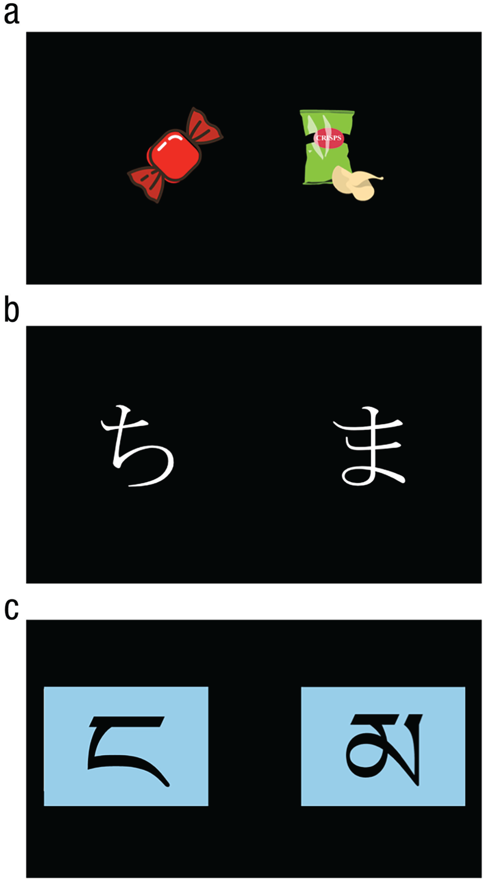
Binary-choice paradigms presented to participants in the studies from which the present data sets were drawn. In the paradigm for Data Sets 1 through 4 (a), participants made choices between two snack foods. In the paradigm for Data Set 5 (b), participants chose between two hiragana symbols with different probabilities of reward. In the paradigm for Data Set 6 (c), participants chose between two Tibetan symbols with probabilities of reward that drifted over time.

There are a few notable differences between the food-choice and probabilistic tasks. In the food-choice tasks (Data Sets 1–4), every trial was a choice between a unique pair of food items. There were many different food items presented to participants in each study, ranging from 70 (in Data Set 1) to 147 (in Data Set 2), and each choice was different. In the probabilistic tasks (Data Sets 5 and 6), on the other hand, participants encountered far fewer unique choices. In Data Set 5, there were six unique symbols, corresponding to 30 unique choices. Each of these pairs was presented to participants multiple times. In Data Set 6, there were only two pairs of symbols. In each trial, participants saw one pair or the other. Although the symbols remained the same throughout the experiment, each symbol’s probability of yielding a reward drifted randomly over the course of the experiment.

In the food-choice tasks, participants received their chosen food from one random trial, so there was no objectively correct choice, whereas in the probabilistic tasks, there was an objectively “correct” option, namely, the symbol with the higher probability of reinforcement. In the Konovalov and Krajbich (2016) study, the reinforcement was a constant monetary reward, whereas in the Cavanagh et al. (2014) study, there was no feedback; participants learned about the stimuli in a separate training task. Finally, in the Konovalov and Krajbich study, participants first made a choice between the same two stimuli. That choice probabilistically led to one of two possible second-stage pairs of stimuli. It is these second-stage decisions that we analyze here, because Konovalov and Krajbich established that the first-stage choices were often governed by a different choice process. We highlight these differences to point out that it would not be surprising to find some variation in the decision process across experiments.

For each of the four binary-food-choice studies (Data Sets 1–4; see Fig. 1a), participants were first asked to rate the desirability of a variety of snack foods on a scale. They then made a series of incentivized choices between two positively rated foods. For the symbolic-reward studies (Data Sets 5 and 6; see Figs. 1b and 1c), participants made choices between symbols that yielded probabilistic rewards. Participants ostensibly knew the probabilities of reward associated with the symbols from feedback. Participants gave written informed consent for all of the studies, and we complied with all relevant ethical regulations. We collected Data Sets 2 through 4 and 6 using an EyeLink 1000 Plus eye tracker (SR Research, Ottawa, Ontario, Canada) at The Ohio State University, with the approval of The Ohio State Institutional Review Board. Below are specific details about each of the studies (for additional details, see Table S7 in the Supplemental Material available online).

Data Set 1

These data come from the study by Krajbich et al. (2010). After rating 70 different food items on a scale from −10 to 10, participants (N = 39) made 100 choices among non-negatively rated (rating ≥ 0) foods with a maximum absolute-value difference of 5 (in a few rare cases, this range was wider, but as in the original article, we excluded these trials from analysis). The Caltech Committee for the Protection of Human Subjects Institutional Review Board approved the experiment.

Data Set 2

Participants (N = 44) in this study (Smith & Krajbich, 2018) rated 147 food items on a scale from −10 to 10 before making 200 choices among positively rated foods (rating > 0). The maximum absolute-value difference for any trial was 5. Participants in this study also completed three other multiattribute choice tasks (200 trials each, 1 involving gambles between the same foods) and another unrelated task at the end of the experiment. Participants had to look at a central fixation cross for 1 s in order for each trial to begin.

We selected food items for each trial according to the following rules: (a) No item was used in more than 7 trials, and (b) the maximum absolute rating difference was 5. For each participant, 10,000 potential trials for the task were generated. Trials that did not fulfill criteria (a) and (b) were discarded. Some participants (n = 22) did not have enough positively rated food items to generate 200 valid trials, so these participants completed as many constraint-satisfying trials as were generated (M = 171.3). Participants earned a $5 show-up fee, additional money from the other tasks, and a chosen food from 1 random trial.

Data Set 3

Participants (N = 44) in this study (Chen & Krajbich, 2016) rated 139 food items on a scale from −10 to 10 and then made 200 choices among nonnegatively rated foods (rating ≥ 0). At the conclusion of each trial, the next trial would begin only after the participant had stared at the central fixation cross for 1 s. The images in this study were designed to be isoluminant.

We selected the items for each trial according to the following rules: (a) No item was used in more than six trials, and (b) the maximum absolute rating difference was 3. An algorithm was used after the rating task and before the choice task to ensure that criteria (a) and (b) could be satisfied. If they were not, then we increased the maximum number of repetitions to seven (n = 7) or eight (n = 3). Participants received a $15 show-up fee and their chosen food from one random trial.

Data Set 4

Participants (N = 36) in this study (Gwinn & Krajbich, 2016) first made a binary yes/no decision about whether they would eat each of 147 food items (the same items as in Data Set 2). Next, they rated each “yes” food item on a scale from 0 to 10 and indicated their confidence in this rating on a scale from 0 to 7. Last, they made 200 choices among the positively rated foods (rating > 0). The maximum absolute-value difference for these choices was 1. We required participants to look at the central fixation cross for 1 s before making each choice. At the end of the study, participants rated each item a second time.

An algorithm generated 200 choices that minimized the number of times any item was seen (for a given participant) while also preserving the maximum absolute-value difference of 1. Participants received $15 for participating and their chosen food from one random trial.

Data Set 5

These data come from the study by Cavanagh et al. (2014; see Fig. 1b). In an initial training phase, participants (N = 20) faced three possible stimulus pairs with the following probabilities of being the correct choice: A:B (80%:20%), C:D (70%:30%), and E:F (60%:40%). After learning to choose the higher probability stimulus in each pair, participants proceeded to the test phase. In that phase, they chose between all possible pairings of the stimuli for 240 trials. The Brown University Institutional Review Board approved this experiment.

Data Set 6

This study (Konovalov & Krajbich, 2016; see Fig. 1c) involved two-stage decisions. In every trial, participants (N = 45) first chose between the same two symbols. Each symbol led to one second-stage state 70% of the time and the other 30% of the time. Each of these two second-stage states had its own two symbols, each with a continuously and independently drifting probability of reward. We used these 150 second-stage choices for our analysis. We did not use the first-stage choices because Konovalov and Krajbich found evidence that many participants were making these decisions before trial onset and thus were not using an SSM choice process.

Sample size and data exclusions

Data Set 1 (Krajbich et al., 2010) used 39 participants. Because the crux of that study was the group-level computational modeling of choices, fixations, and RTs, the 100 choices made by each participant yielded plenty of data with which to conduct the primary modeling analyses. Data Sets 2 through 4 and 6 are similar in style to those reported in the Krajbich et al. article and had similar modeling goals, so their sample sizes of 44, 44, 36, and 45, respectively, were modeled after the original study. Data Set 5 was collected in a different lab, so we did not have a say in the sample size.

We were unable to collect data from some participants because of computer crashes, corrupted data files, inability to calibrate the eye tracker, or too many negative food ratings (in Data Sets 1–4) to generate choices. A priori, we excluded excessively fast decisions—that is, greater than 250 ms—and excessively slow decisions—that is, more than 2 standard deviations above participant-level means, using log(RT)—from analysis in all data sets because they were probably due to accidental button presses, the participant intentionally skipping the trial, or distraction. This resulted in the exclusion of 144, 303, 347, 245, 203, and 147 trials for Data Sets 1 through 6, respectively, corresponding to 3% to 4% of trials. Other than this RT exclusion criterion, we used all of the data in the initial data sets provided to us.

Computational models

Both models discussed here are extensions of the DDM (Ratcliff, 1978). That is, they both rely on a noisy sequential-sampling process, by which relative evidence for the two alternatives is accumulated. When the evidence in favor of one alternative (relative to the other) reaches a predefined boundary, the decision is made. The average rate of evidence accumulation is called the drift rate (ν) and depends on the difference in value between the two alternatives. There are a number of other essential parameters in the DDM: within-trial variability in drift rate (σ), nondecision time (t_er), and boundary separation (a). For the model to be identifiable, ν, σ, or a must be fixed. Therefore, in the current analysis, we fixed boundary separation to 2, as in the study by Krajbich et al. (2010), and estimated the remaining parameters (plus the attentional parameters: θ and η). These models differ from the traditional DDM because they incorporate the effects of attention on choice. More specifically, both models assume that the drift rate changes with each shift in gaze. However, the models differ in how this change occurs.

The multiplicative model (aDDM; Krajbich et al., 2010) assumes that attention to one alternative results in the discounting of the value of the other alternative for the duration of the gaze. So, the drift rates (ν) in the aDDM are as follows:

gaze left : ν = d (U_{L} - θ U_{R})

gaze right : ν = d (θ U_{L} - U_{R})

Here, U_L and U_R are the subjective values (i.e., utilities) of the left and right alternatives, respectively, d is a scaling parameter for the values, and $θ$ is the multiplicative attentional discounting parameter. Specifically, it discounts the value of the item not looked at by a fraction of this item’s value.

On the other hand, the additive model assumes that attention to one alternative simply adds momentary evidence for that option. Thus, the drift rates in the additive model are as follows:

gaze left : ν = d (U_{L} - U_{R} + η)

gaze right : ν = d (U_{L} - U_{R} - η)

Here, the attentional effects are captured with the parameter η, which adds a fixed boost to the looked-at alternative, regardless of its value. The consequences of these differences play out in the evidence-accumulation process. Specifically, the multiplicative model demonstrates more drastic shifts in the drift rate for choices between options with higher values, whereas the additive model’s drift-rate shifts are constant (see Fig. 2). We fitted both models to all six data sets. See the Supplemental Material for more information.

Fig. 2.

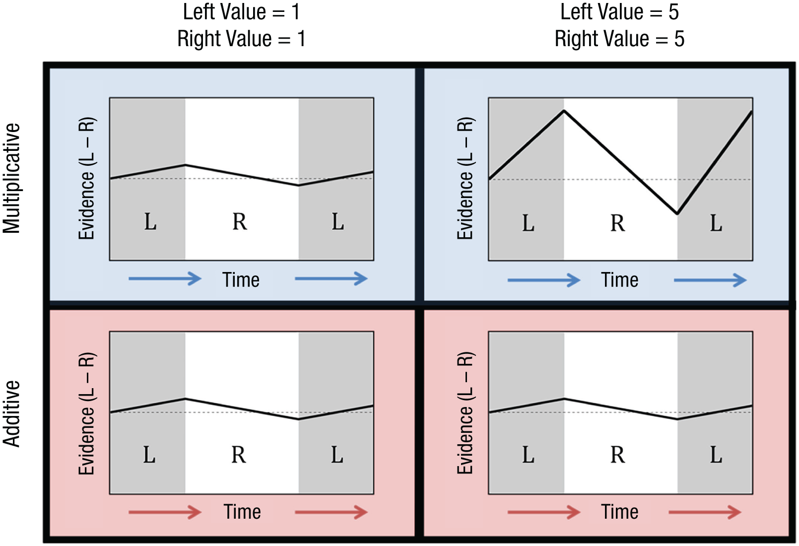
Illustration of the effects of attention on the choice process, separated by model (multiplicative and additive) and overall value (left value + right value). In the multiplicative model, higher overall value leads to greater shifts in the drift rate (i.e., slope of the black line) as gaze shifts back and forth between the left (L) and right (R) alternatives. On the other hand, the additive model does not predict any difference in the drift-rate shifts for high versus low overall value.

Results

RT versus overall value

The two models (multiplicative and additive) differ in their predictions about how the overall value of the alternatives should influence the time it takes to respond. The drift rates in the additive model, as in the standard DDM, depend only on the difference in values (see Fig. 2). When analyses control for value difference, the overall value should have no effect on the decision because all that matters is the net evidence (given by the difference in value between the alternatives); evidence for one option is evidence against the other.

Conversely, in the multiplicative-attention model, the overall value of the alternatives does matter. The higher the values, the bigger the change in drift rate when gaze shifts from one alternative to the other. For example, the standard DDM suggests equal drift rates for a choice between two options with a value of 1 and a choice between two options with a value of 5; in both cases, the drift rate is 0. In the DDMs with attention, there are two possible drift rates, depending on the gaze location, which average out to the same drift rate as in the standard DDM. In the additive-attention model, the drift rates in both of these trials are ±η. In the multiplicative-attention model, the drift rates are ±(1 – θ) and ±(5 – 5θ), respectively. Because of this difference in the magnitudes of the drift rates in the multiplicative model, the latter trials will generally reach a boundary more quickly, resulting in shorter RTs (see Fig. 2). Thus, the multiplicative model, but not the additive model, predicts faster decisions for higher overall values.

To verify this prediction, we simulated data sets with both models (for more details, see the Supplemental Material), using choice problems from Data Set 2 and parameters taken from the study by Krajbich et al. (2010), and estimated the following regression model:

\log (R T) ~ β_{0} + β_{1} | U_{L} - U_{R} | + β_{2} (U_{L} + U_{R}) .

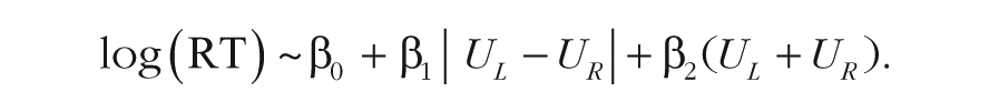
The coefficient β₂ is the primary variable of interest, but it is important to account for the difference in value between the two alternatives because participants decide faster in scenarios with higher value differences.

As expected, the multiplicative-model simulations displayed a negative relationship between RT and overall value (β₂ = −0.013 s per rating, 95% confidence interval, or CI = [−0.014, −0.012], p < .001), whereas the additive-model simulations did not (β₂ = −0.0004 s per rating, 95% CI = [−0.001, 0.0003], p = .299; see Figs. 3a and 3b). Without taking value difference into account, the additive-attention model exhibits a relationship between RT and overall value that is U shaped because extreme overall values correspond to small value differences.

Fig. 3.

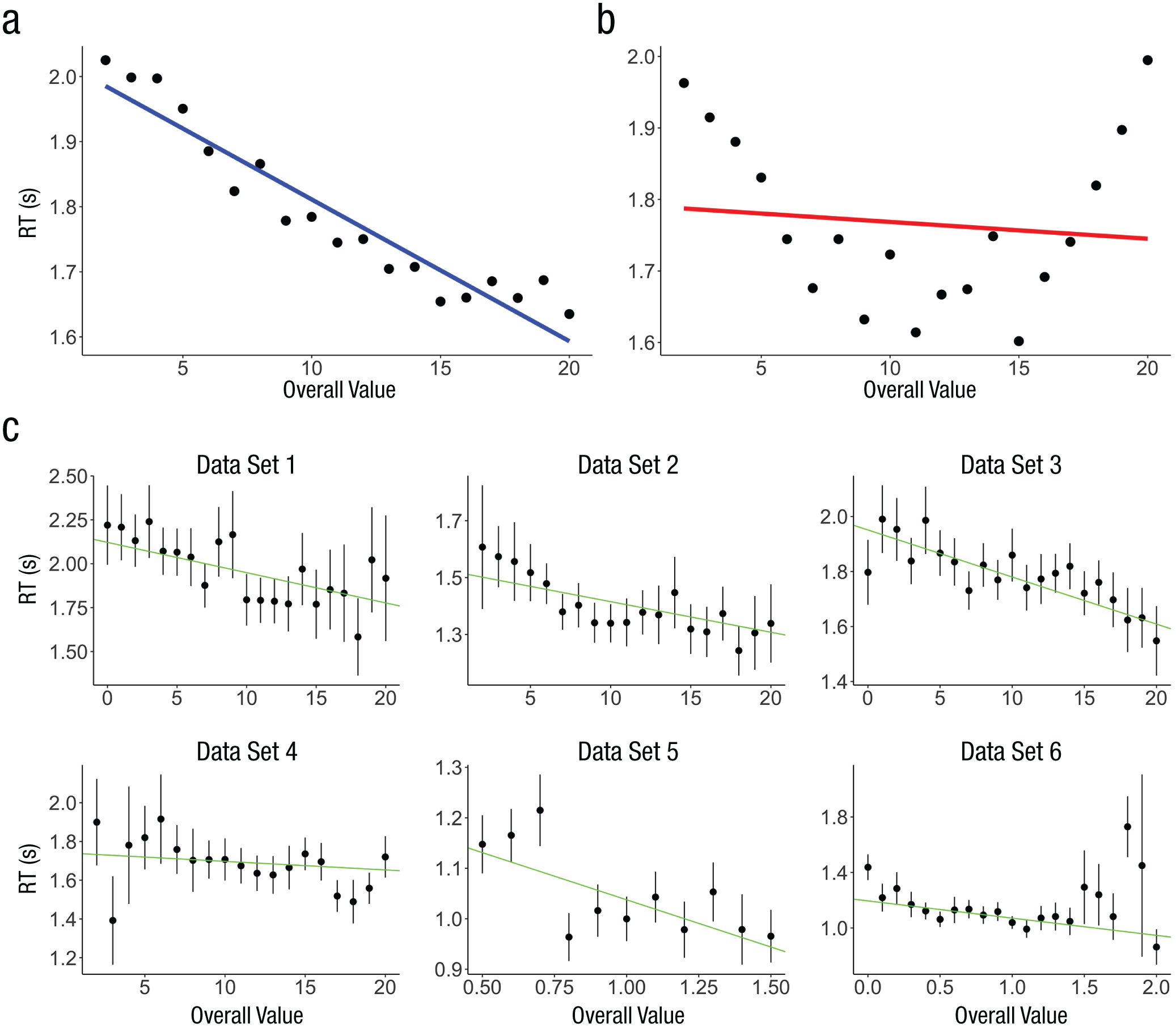
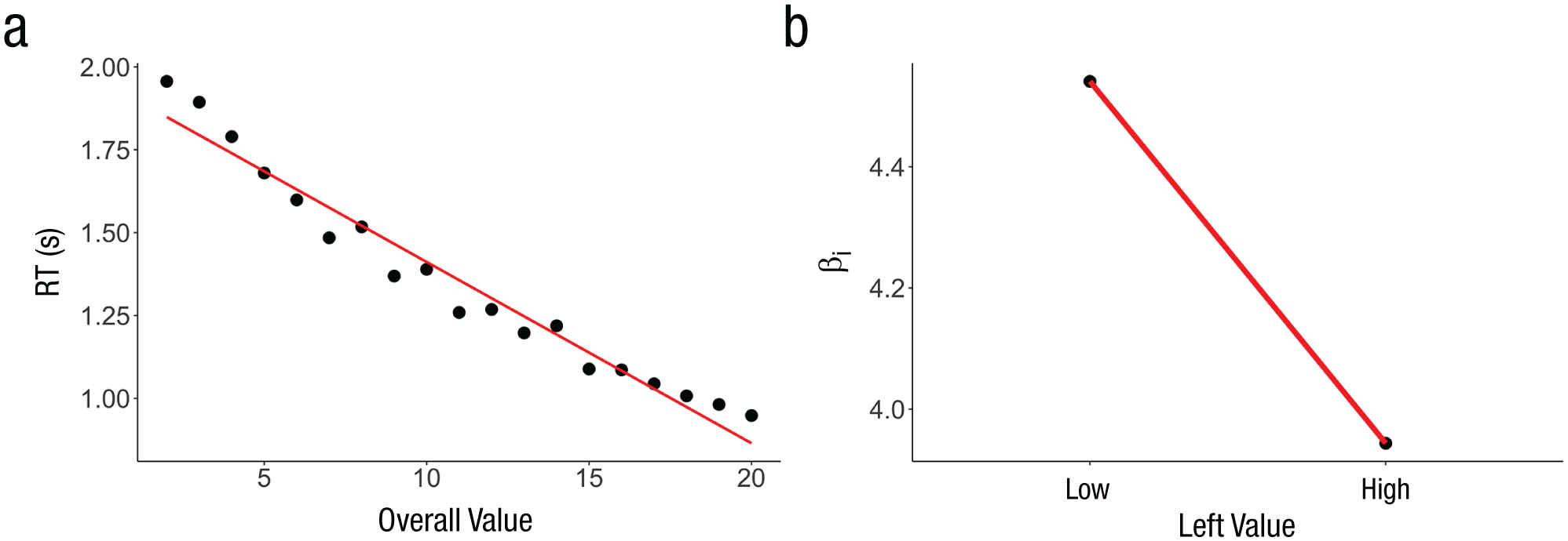
Predictions of the multiplicative model and additive model about the relationship between overall value (left value + right value) and average response time (RT), as well as results from the actual data. The multiplicative model (a) predicts a decrease in RT as overall value increases, as a result of larger shifts in the drift rate. In the additive model (b), the drift rate depends only on the value difference, so the shortest RTs occur in situations with higher value differences. In these simulated data, based on choice problems from Data Set 2, the trials with the lowest and highest overall values have very small value differences, which create the U shape. The relationship between overall value and RT (c) is shown separately for each of the data sets (Ns = 39, 44, 44, 36, 20, and 45 for Data Sets 1 to 6, respectively). In all panels, black circles are data points—simulated data in (a) and (b) and actual data in (c)—and error bars show standard errors of the mean across participants. The blue, red, and green lines are simple linear regressions fitted to the data. For the parameters used to generate data in (a) and (b), see the Supplemental Material available online.

Next, we examined the relationship between RT and overall value in the data (see Fig. 3c). We estimated full mixed-effects versions of the same model from above, for each of the six data sets. As in the multiplicative-attention simulations, we found significantly negative β₂ coefficients in every case, indicating that an increase in overall value (U_L + U_R) corresponds to a decrease in RT (see Table 1). Remarkably, after rescaling the values from Data Sets 5 and 6 to the same range (0–10) as in Data Sets 1 through 4, the average β₂ coefficient across studies was −0.011 s per rating, compared with −0.013 s per rating in the simulations. Similarly, when we used all data sets in one analysis (with variables standardized at the data-set level), we found that the relationship between overall value and logged RT was significantly negative (mixed-effects model: β₂ = −0.122, 95% CI = [−0.142, −0.101], p < .001).

Table 1.

Results of the Regressions on the Relationship Between Overall Value and Response Time

Data set	b₂	95% CI	t
1	−0.013	[−0.019, −0.008]	−4.78
2	−0.009	[−0.013, −0.006]	−5.47
3	−0.010	[−0.012, −0.008]	−8.36
4	−0.005	[−0.008, −0.003]	−3.92
5	−0.202	[−0.284, −0.119]	−4.87
6	−0.178	[−0.249, −0.111]	−5.21

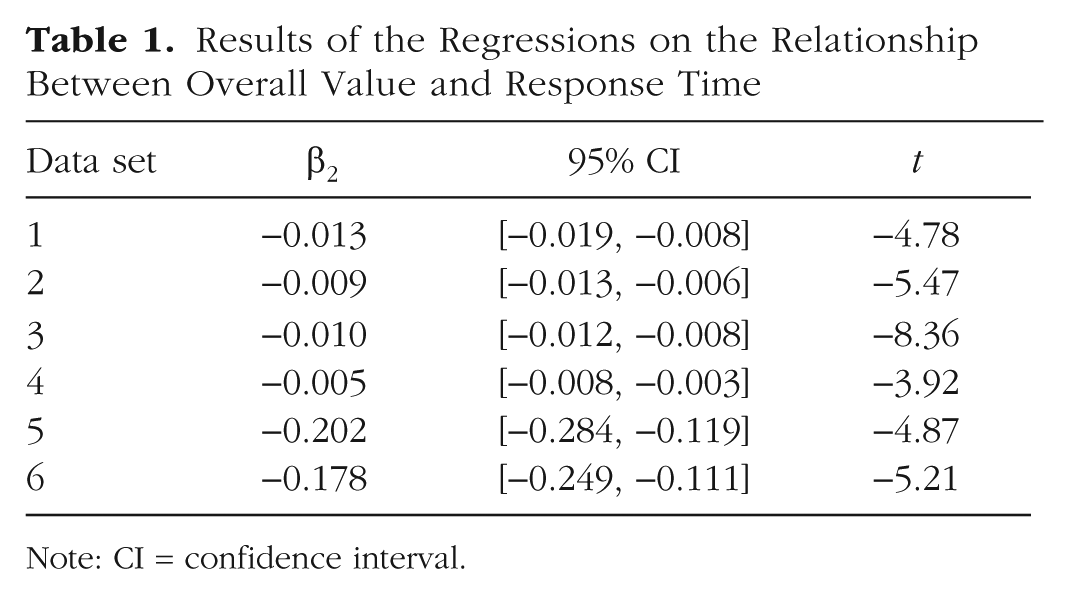
Note: CI = confidence interval.

To more directly test the relationship between overall value and RT, we ran a similar mixed-effects regression but used only the trials with a value difference equal to zero (the data from Cavanagh et al., 2014, did not have any trials of this nature, so we did not run this analysis on that data set). This allowed us to discard the value-difference variable, simplifying the model:

\log (R T) ~ β_{0} + β_{1} (U_{L} + U_{R}) .

The negative β₁ coefficient in every data set, significant in four out of five (see Table 2), confirmed the inverse relationship between overall value and RT, providing additional support for a multiplicative role of attention on choice.

Table 2.

Results of the Regressions on the Relationship Between Overall Value and Response Time in Trials With a Value Difference Equal to 0

Data set	b₁	95% CI	t
1	−0.007	[−0.017, 0.002]	−1.60
2	−0.009	[−0.015, −0.004]	−3.38
3	−0.006	[−0.009, −0.003]	−3.59
4	−0.005	[−0.009, −0.0002]	−2.06
6	−0.246	[−0.364, −0.138]	−4.48

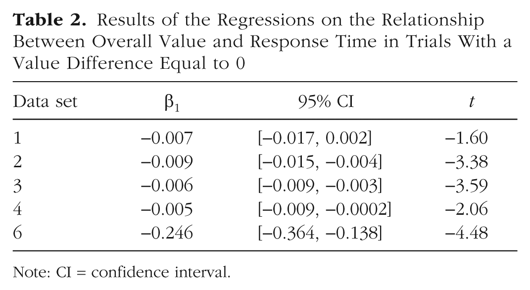
Note: CI = confidence interval.

These results were also replicated at the individual level. A mean of 81% (87%, 84%, 86%, 67%, 85%, and 77% in Data Sets 1–6, respectively) of the participants exhibited a negative relationship between overall value and logged RT, after we controlled for absolute-value difference (as in Table 1). The remaining participants (who did not have a negative relationship between overall value and RT) did not align well with the additive model either, generally showing a positive or flat relationship between overall value and RT, rather than the parabolic shape seen in Figure 3b.

Modeling the value–attention interaction

Another way to test for the mechanism driving the effects of attention on choice is to model the interaction between value and gaze. According to the multiplicative model, attention to options with greater value should have a greater influence on choices, relative to attention to options with lower value. The additive model, on the other hand, posits that the value of the gazed-at option should not influence the effect of attention on choice. Returning to our earlier example (see Fig. 2), one can see that the shift in drift rates due to attention is constant in the additive model but increases with overall value in the multiplicative model.

To verify this prediction, we used the same simulations from before and regressed choice outcome (choose left) on the value difference (U_L – U_R) between the items, the overall value (U_L + U_R), and the left-dwell proportion (dwell time for the left option as a fraction of total dwell time) separated into two cases: one with the left value less than the median value in the group data set and one with the left value greater than or equal to the median value in the group data set. In other words, in each trial, only one of the left-dwell-proportion variables had a nonzero value. More explicitly, we estimated the following logistic model:

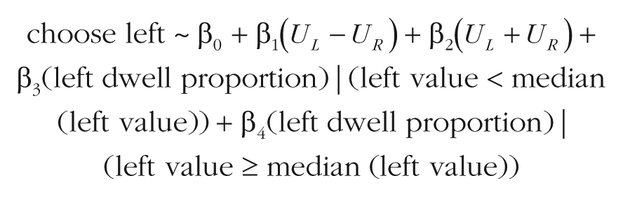
\begin{matrix} choose left ~ β_{0} + β_{1} (U_{L} - U_{R}) + β_{2} (U_{L} + U_{R}) + \\ β_{3} (left dwell proportion) | (left value < median \\ (left value)) + β_{4} (left dwell proportion) | \\ (left value \geq median (left value)) \end{matrix}

Then, we plotted the values of β₃ and β₄ (see Figs. 4a and 4b). The multiplicative model, as expected, showed a smaller left-dwell-proportion coefficient for low values (β₃ = 5.423) than for high values (β₄ = 7.029), as shown by the nonoverlapping 95% CIs (95% CI for β₃ = [5.292, 5.554]; 95% CI for β₄ = [6.868, 7.191]). The additive model, on the other hand, had equivalent coefficients for low values (β₃ = 5.750) and high values (β₄ = 5.757), as shown by the nearly indistinguishable 95% CIs (95% CI for β₃ = [5.602, 5.900]; 95% CI for β₄ = [5.584, 5.932]).

Fig. 4.

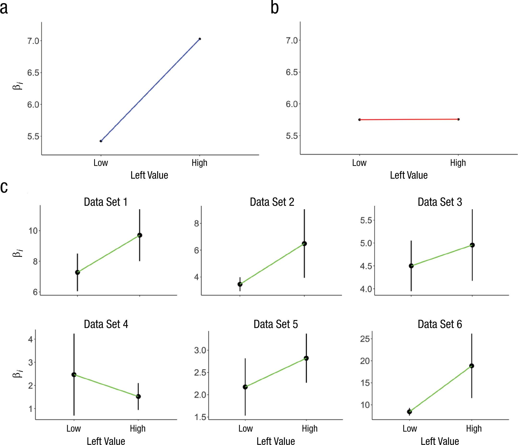
Predictions of the multiplicative model and additive model about the effects of the interaction between attention and value on choice, as well as results from the actual data. The multiplicative model (a) predicts an increasing effect of attention on the choice process (β_i) as the value of the looked-at alternative increases, whereas the additive model (b) predicts that the influence of attention is constant, regardless of the value of the looked-at alternative. The relationship between choice and the interaction between attention and value (c) is shown separately for each of the data sets (Ns = 39, 44, 44, 36, 20, and 45 for Data Sets 1–6, respectively). In all panels, black circles are data points—simulated data in (a) and (b) and actual data in (c)—and error bars show standard errors of the mean across subjects. See the Supplemental Material available online for odds-ratio results (see Fig. S6) and for parameters used to generate data in (a) and (b). Participants who did not have enough observations in either the low- or high-value bin to generate a coefficient were excluded from this analysis (n = 6 across all data sets).

We observed a positive difference between high and low values in five out of six data sets (see Fig. 4c). Results of one-tailed paired-samples t tests on each individual data set were mostly marginal or nonsignificant—Data Set 1: t(37) = 1.99, p = .027; Data Set 2: t(43) = 1.20, p = .119; Data Set 3: t(43) = 0.74, p = .233; Data Set 4: t(32) = −0.57, p = .713; Data Set 5: t(19) = 1.00, p = .166; Data Set 6: t(42) = 1.44, p = .079. Combined, however, they revealed a significant difference in the expected direction, t(221) = 2.25, p = .013.

Estimating the effect of attention with a median split allowed us to avoid imposing the assumption that value had a linear effect on the relationship between dwell proportion and choice. However, we also ran a simpler linear interaction model at the individual level for each data set. The results of this analysis support a multiplicative effect in the food-choice studies but not the learning studies (see Fig. S7 in the Supplemental Material).

Alternative additive model with value-contingent bounds

The two models discussed so far have the same number of parameters and are therefore easily comparable. However, Cavanagh et al. (2014) found that their model fitted better when allowing for trial-level, value-related changes in the boundary separation during the model-fitting process. Note that in diffusion modeling, researchers typically assume that the decision boundaries do not vary as a function of the choice options but rather as a function of time pressure, speed/accuracy instructions, and so on (Ratcliff & McKoon, 2008). Nevertheless, we simulated an additive model with boundaries that linearly decrease to one half the original separation across the range of overall values (i.e., the boundaries were set to ±1 for overall value = 2 and ±0.5 for overall value = 20). More details about this alternative model can be found in the Supplemental Material. With these boundaries, the additive model can account for the inverse relationship between overall value and RT (see Fig. 5; β = −0.0384, 95% CI = [–0.0392, –0.0377], p < .001).

Fig. 5.

Results from the alternative version of the additive model with tighter bounds for higher overall value. The scatterplot (a) shows the relationship between average response time (RT) and the overall value of the options. Thus, the model can account for the inverse relationship between overall value and RT. Attentional-influence coefficients (using the same model as in Fig. 4) are plotted in (b) against the values of the gazed-at option. According to this model, attention to higher valued alternatives corresponds to a lesser effect on choice. Thus, this alternative model cannot account for the positive interaction between value and the effect of attention observed in the data (see Fig. 4). In each plot, the black dots are model-generated simulations (see the Supplemental Material available online), and the red line is a simple fitted regression line through the simulations.

However, this alternative model did not yield the same interaction between value and gaze as in the multiplicative model and data (see Fig. 4). In fact, the interaction was negative with this alternative model (see Fig. 5); thus, it is refuted by the data. We do acknowledge that this is only one example of value-dependent boundaries, but it does serve as an illustrative tool. What matters is that when the boundaries were tighter, we saw a smaller effect of gaze on choice with the additive model (see Fig. S4 in the Supplemental Material). Therefore, an additive model in which the boundaries tighten with higher overall value cannot account for the positive value-attention interaction observed in the data.

Modeling results

The previous analyses highlight key differences between the additive and multiplicative attention DDMs and indicate an advantage for the multiplicative model. However, it is important to note that the two models otherwise provide quite similar fits to the data. To see this, we fitted all of the data sets with the additive and multiplicative models (see the Supplemental Material). Both models can account for some overarching trends in the data (see Fig. 6). For instance, both display the inverse relationship between RT and value difference, and both capture the tendency for participants to choose the last option that they looked at (Konovalov & Krajbich, 2016; Krajbich et al., 2010).

Fig. 6.

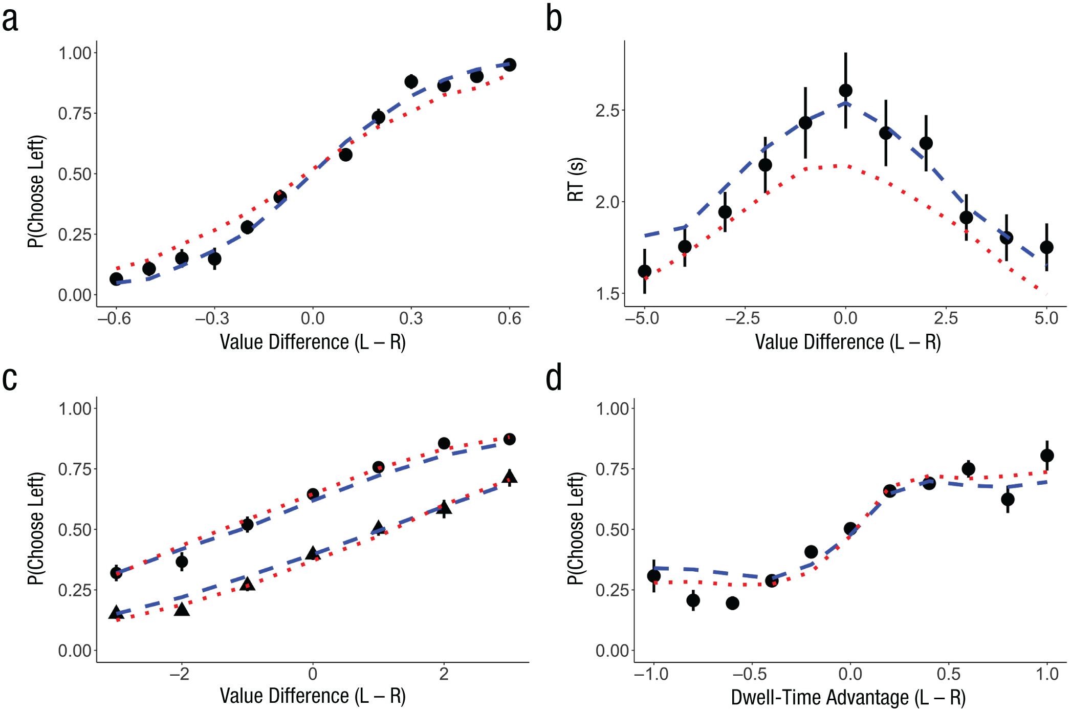
Examples of the effects that both the additive and multiplicative models can explain. Both models can predict (a) choice proportions as a function of the value difference between the options (here, in Data Set 5, N = 20). Both models predict (b) the inverse relationship between response time (RT) and the absolute-value difference observed in the data, in which the fastest decisions are those with the highest absolute-value difference, and the slowest decisions are those with the lowest absolute-value difference (here, in Data Set 1, N = 39). Both models predict (c) a last-look bias, such that participants are more likely to choose the last option they look at, unless the last-seen option is sufficiently worse than the alternative (here, in Data Set 3, N = 44). Both models predict (d) an increase in choice probability as the relative dwell time for an option increases (here, in Data Set 2, N = 44). In all panels, the black symbols are data points (with standard errors of the mean across participants), the blue dashed line is the best-fitting multiplicative model (see the Supplemental Material available online), and the red dotted line is the best-fitting additive model (see the Supplemental Material). L = left, R = right.

It is natural to want to compare the models on the basis of overall goodness of fit. However, such comparisons may depend on how these statistics are calculated. Even with standard DDM fitting, there are a variety of methods, and in our setting, we wished to account for the eye-tracking data. One method, in which we conditioned the data on whether the participant looked at the chosen item last, yielded roughly equivalent fits for the two models (see Tables S2 and S3 in the Supplemental Material). Another method, conditioning the data on dwell-time differences, yielded better fits for the multiplicative model (see Tables S4 and S5 in the Supplemental Material). It is important to note that neither of these methods conditioned the data on overall value during the fitting process.

To additionally investigate the attention–value interaction, in line with the study by Cavanagh et al. (2014), we estimated several models using a hierarchical drift diffusion model (HDDM; Wiecki, Sofer, & Frank, 2013). The HDDM analyses confirmed multiplicative effects for Data Sets 1 through 4 with Bayesian posterior probabilities of 1, .993, 1, and .9885, respectively. On the other hand, the results were more equivocal for the learning tasks (Data Sets 5 and 6), with a Bayesian posterior probability of .391 for multiplicative effects in Data Set 5 and either .025 or 1 in Data Set 6, depending on whether we used subjective or objective values in the model. For further information on these analyses, see the Supplemental Material.

Discussion

In this article, we presented two ways in which gaze might influence the decision process. Gaze might provide a constant bias in favor of the attended option (additive model), or it might amplify the value of that option (multiplicative model). Using six different data sets from multiple labs and using multiple paradigms, we found substantial evidence in favor of multiplicative effects. Specifically, attention to a given alternative interacts with the value of said alternative such that gaze to higher valued options has a greater influence on choice than gaze to lower valued options. This relationship was most evident in tasks using large sets of familiar stimuli, compared with small sets of learned stimuli.

One finding that distinguishes between the two proposed mechanisms (additive and multiplicative) is the inverse relationship between overall value and RT. This highlights that RTs are not simply a function of the value differences (as is often assumed; e.g., Ashby et al., 2016). These factors need to be accounted for in model comparisons. In the multiplicative model (the aDDM; Krajbich et al., 2010), the average drift rate is a function of not only the difference in value between the options but also the values themselves. The simple additive model, on the other hand, cannot account for this finding because the drift rate is purely a function of the difference in value between the two alternatives. Some other SSM frameworks (Lo & Wang, 2006; Ratcliff, Voskuilen, Teodorescu, 2018; Usher & McClelland, 2001) do predict faster decisions for higher overall value, but they do not account for the relationship between gaze and choice.

The interaction between value and the effect of attention was generally positive and, overall, significant in the data sets that we examined. The aDDM and the additive model differ in their predictions about this relationship: While the aDDM predicts a positive value–attention interaction, the additive model predicts a constant effect of attention, regardless of the value of the looked-at option.

It is worth briefly discussing the three data sets with the weaker effects of overall value on attentional influence. Data Set 4 was from an experiment investigating the role of attitude accessibility and confidence on the choice process. Participants were exposed to each item many times, and so they may have had more well-formed preferences than is typical. In Data Sets 5 and 6, participants saw very few stimuli (six in each choice task). In Data Set 5, the values of these stimuli were learned in a prior training task, whereas in Data Set 6, the values of the stimuli varied over time.

Data Set 5 was originally found to support the additive model rather than the multiplicative model, on the basis of HDDM fits (Cavanagh et al., 2014). Our own fits to those data yielded more equivocal results. For instance, the analysis shown in Figure 4 suggests a slightly positive interaction in this data set, whereas our supplemental interaction analysis (see Fig. S7) suggests a slightly negative interaction. Visualizations of the effect of dwell time on choice (see Fig. S1 in the Supplemental Material) show multiplicative effects for large value differences but not for small value differences. Similarly, one model-fitting technique (HDDM) slightly favored the additive model, whereas the others (DDM) favored the multiplicative model. The discrepancy could be due to the assumptions of each fitting method, especially if these data were not all generated by a diffusion-model process, which is a concern given the small number of unique trials.

On a similar note, Data Set 6 was used by its original authors (Konovalov & Krajbich, 2016) to argue that participants in that task often knew ahead of time what they were going to choose and so may not have always been using a DDM process. It is not a surprise, then, that the multiplicative effects of attention are somewhat obscured in this data set.

Although our results support a multiplicative effect, we have not yet ruled out the possibility that there are also additive effects. There are a few ways to address this issue. One way to rule out the additive effect is to examine the main effect of dwell proportion, which in our model corresponds to the case in which the value is equal to 0 and thus captures a pure additive effect. Regression results here revealed a significant additive effect in four of the six data sets (see Fig. S7). A second way to check for additive effects is with formal DDM fits. The results from these analyses also suggest that there may be additive gaze effects (see Table S6 in the Supplemental Material). There are caveats to these results, though. As mentioned above, the multiplicative model assumes no effect of gaze on choice for zero-value items. This means that arbitrary shifts in the value scale will affect the main effect of dwell proportion and change how well the multiplicative model fits the data. The goodness of fit for the multiplicative model (but not the additive model) will worsen if the measured zero point does not correspond exactly to the true zero point. What this means is that a main effect of dwell proportion or worse fit for the multiplicative model could simply be due to an incorrect assumption about the zero point on the value scale.

Our findings also allow us to weigh in on the direction of causality between attention and choice. Although some authors have posited that attention drives choices (Armel et al., 2008; Mormann et al., 2012; Pärnamets et al., 2015; Reeck, Wall, & Johnson, 2017; Towal et al., 2013; Zoltak, Veling, Chen, & Holland, 2018), a constant challenge to this assertion is the possibility that attention is merely indicative of emerging preferences (Shimojo, Simion, Shimojo, & Scheier, 2003). This latter explanation seems unlikely given our results. Without the amplifying effects of attention on value, the DDM would require additional ad hoc assumptions to explain why high overall value choices are faster and more strongly tied to gaze.

Ultimately, this research demonstrates that the mechanism underlying the attention–choice link is not a simple boost to the evidence accumulated for the gazed-at option but a more complex interaction that takes into account the values of the options, especially in choices from large sets of familiar stimuli (e.g., food choices). The aDDM is one such model that captures this multiplicative effect. There are likely other instantiations that can account for the patterns discussed in this article, but the aDDM is the simplest extension of the DDM capable of capturing the multiplicative role of attention in choice.

Supplemental Material

KrajbichOpenPracticesDisclosure – Supplemental material for Gaze Amplifies Value in Decision Making

Supplemental material, KrajbichOpenPracticesDisclosure for Gaze Amplifies Value in Decision Making by Stephanie M. Smith and Ian Krajbich in Psychological Science

Supplemental Material

KrajbichSupplementalMaterial – Supplemental material for Gaze Amplifies Value in Decision Making

Supplemental material, KrajbichSupplementalMaterial for Gaze Amplifies Value in Decision Making by Stephanie M. Smith and Ian Krajbich in Psychological Science

Footnotes

Acknowledgements

We thank James Cavanagh, Michael Frank, Antonio Rangel, James Wei Chen, Rachael Gwinn, and Arkady Konovalov for sharing their data.

Action Editor

Timothy J. Pleskac served as action editor for this article.

Author Contributions

I. Krajbich devised the project, cowrote the manuscript, and supervised the project. S. M. Smith performed the analyses and cowrote the manuscript. Both authors approved the final manuscript for submission.

Declaration of Conflicting Interests

The author(s) declared that there were no conflicts of interest with respect to the authorship or the publication of this article.

Funding

We gratefully acknowledge support from the National Science Foundation (Graduate Research Fellowship Program award to S. M. Smith; Career Award 1554837 to I. Krajbich).

Supplemental Material

Additional supporting information can be found at

Open Practices

Data Sets 1 through 4 and 6 are available on the Open Science Framework (OSF) at https://osf.io/ktsye/?view_only=f0b31e6d60e5402c89bb57dfede88c82. Requests for Data Set 5 may be sent to the corresponding author of that project (James Cavanagh; jcavanagh@unm.edu). The computational-modeling code used to generate the analyses in the present study is available at the OSF address above. The design and analysis plans for the present study were not preregistered. The complete Open Practices Disclosure for this article can be found at http://journals.sagepub.com/doi/suppl/10.1177/0956797618810521. More information about the Open Practices badges can be found at .

References

Armel

K. C.

Beaumel

Rangel

(2008). Biasing simple choices by manipulating relative visual attention. Judgment and Decision Making, 3, 396–403.

Ashby

N. J. S.

Jekel

Dickert

Glöckner

(2016). Finding the right fit: A comparison of process assumptions underlying popular drift-diffusion models. Journal of Experimental Psychology: Learning, Memory, and Cognition, 42, 1982–1993. doi:10.1037/xlm0000279

Bakkour

Leuker

Hover

A. M.

Giles

Poldrack

R. A.

Schonberg

(2016). Mechanisms of choice behavior shift using cue-approach training. Frontiers in Psychology, 7, Article 421. doi:10.3389/fpsyg.2016.00421

Bakkour

Lewis-Peacock

J. A.

Poldrack

R. A.

Schonberg

(2017). Neural mechanisms of cue-approach training. NeuroImage, 151, 92–104. doi:10.1016/j.neuroimage.2016.09.059

Busemeyer

Diederich

(2002). Survey of decision field theory. Mathematical Social Sciences, 43, 345–370. doi:10.1016/S0165-4896(02)00016-1

Busemeyer

Townsend

(1993). Decision field theory: A dynamic-cognitive approach to decision making in an uncertain environment. Psychological Review, 100, 432–459. doi:10.1037/0033-295X.100.3.432

Cavanagh

J. F.

Wiecki

T. V.

Kochar

Frank

M. J.

(2014). Eye tracking and pupillometry are indicators of dissociable latent decision processes. Journal of Experimental Psychology: General, 143, 1476–1488. doi:10.1037/a0035813

Chen

W. J.

Krajbich

(2016). Pupil dilation and attention in value-based choice. Unpublished manuscript, The Ohio State University.

Fiedler

Glöckner

(2012). The dynamics of decision making in risky choice: An eye-tracking analysis. Frontiers in Psychology, 3, Article 335. doi:10.3389/fpsyg.2012.00335

10.

Fiedler

Glöckner

Nicklisch

Dickert

(2013). Social value orientation and information search in social dilemmas: An eye-tracking analysis. Organizational Behavior and Human Decision Processes, 120, 272–284. doi:10.1016/j.obhdp.2012.07.002

11.

Fisher

(2017). An attentional drift diffusion model over binary-attribute choice. Cognition, 168, 34–45. doi:10.1016/j.cognition.2017.06.007

12.

Folke

Jacobsen

Fleming

S. M.

De Martino

(2016). Explicit representation of confidence informs future value-based decisions. Nature Human Behaviour, 1, Article 2. doi:10.1038/s41562-016-0002

13.

Gwinn

R. E.

Krajbich

(2016). Attitudes and attention: How attitude accessibility and certainty influence attention and subjective choice. Unpublished manuscript, The Ohio State University.

14.

Hunt

L. T.

Kolling

Soltani

Woolrich

M. W.

Rushworth

M. F. S.

Behrens

T. E. J.

(2012). Mechanisms underlying cortical activity during value-guided choice. Nature Neuroscience, 15, 470–476. doi:10.1038/nn.3017

15.

Konovalov

Krajbich

(2016). Gaze data reveal distinct choice processes underlying model-based and model-free reinforcement learning. Nature Communications, 7, Article 12438. doi:10.1038/ncomms12438

16.

Krajbich

Armel

Rangel

(2010). Visual fixations and the computation and comparison of value in simple choice. Nature Neuroscience, 13, 1292–1298. doi:10.1038/nn.2635

17.

Krajbich

Camerer

Rangel

(2012). The attentional drift-diffusion model extends to simple purchasing decisions. Frontiers in Psychology, 3, Article 193. doi:10.3389/fpsyg.2012.00193

18.

Krajbich

Rangel

(2011). Multialternative drift-diffusion model predicts the relationship between visual fixations and choice in value-based decisions. Proceedings of the National Academy of Sciences, USA, 108, 13852–13857. doi:10.1073/pnas.1101328108

19.

Krajbich

Smith

S. M.

(2015). Modeling eye movements and response times in consumer choice. Journal of Agricultural & Food Industrial Organization, 13(1), 55–72. doi:10.1515/jafio-2015-0016

20.

Lim

S.-L.

O’Doherty

J. P.

Rangel

(2011). The decision value computations in the vmPFC and striatum use a relative value code that is guided by visual attention. The Journal of Neuroscience, 31, 13214–13223.

21.

C.-C.

Wang

X.-J.

(2006). Cortico–basal ganglia circuit mechanism for a decision threshold in reaction time tasks. Nature Neuroscience, 9, 956–963. doi:10.1038/nn1722

22.

Mormann

M. M.

Navalpakkam

Koch

Rangel

(2012). Relative visual saliency differences induce sizable bias in consumer choice. Journal of Consumer Psychology, 22(1), 67–74. doi:10.1016/j.jcps.2011.10.002

23.

Pärnamets

Johansson

Hall

Balkenius

Spivey

M. J.

Richardson

D. C.

(2015). Biasing moral decisions by exploiting the dynamics of eye gaze. Proceedings of the National Academy of Sciences, USA, 112, 4170–4175.

24.

Pirrone

Azab

Hayden

B. Y.

Stafford

Marshall

J. A. R

. (2018). Evidence for the speed–value trade-off: Human and monkey decision making is magnitude sensitive. Decision, 5, 129–142. doi:10.1037/dec0000075

25.

Polanía

Krajbich

Grueschow

Ruff

C. C.

(2014). Neural oscillations and synchronization differentially support evidence accumulation in perceptual and value-based decision making. Neuron, 82, 709–720. doi:10.1016/j.neuron.2014.03.014

26.

Ratcliff

(1978). A theory of memory retrieval. Psychological Review, 85, 59–108. doi:10.1037/0033-295X.85.2.59

27.

Ratcliff

Voskuilen

Teodorescu

(2018). Modeling 2-alternative forced-choice tasks: Accounting for both magnitude and difference effects. Cognitive Psychology, 103, 1–22.

28.

Ratcliff

McKoon

(2008). The diffusion decision model: Theory and data for two-choice decision tasks. Neural Computation, 20, 873–922.

29.

Reeck

Wall

Johnson

E. J.

(2017). Search predicts and changes patience in intertemporal choice. Proceedings of the National Academy of Sciences, USA, 114, 11890–11895. doi:10.1073/pnas.1707040114

30.

Schonberg

Bakkour

Hover

A. M.

Mumford

J. A.

Nagar

Perez

Poldrack

R. A.

(2014). Changing value through cued approach: An automatic mechanism of behavior change. Nature Neuroscience, 17, 625–630. doi:10.1038/nn.3673

31.

Shimojo

Simion

Shimojo

Scheier

(2003). Gaze bias both reflects and influences preference. Nature Neuroscience, 6, 1317–1322. doi:10.1038/nn1150

32.

Smith

S. M.

Krajbich

(2018). Attention and choice across domains. Journal of Experimental Psychology: General. Advance online publication. doi:10.1037/xge0000482

33.

Stewart

Hermens

Matthews

W. J.

(2016). Eye movements in risky choice. Journal of Behavioral Decision Making, 29, 116–136. doi:10.1002/bdm.1854

34.

Towal

R. B.

Mormann

Koch

(2013). Simultaneous modeling of visual saliency and value computation improves predictions of economic choice. Proceedings of the National Academy of Sciences, USA, 110, E3858–E3867.

35.

Usher

McClelland

J. L.

(2001). On the time course of perceptual choice: The leaky competing accumulator model. Psychological Review, 108, 550–592.

36.

Vaidya

A. R.

Fellows

L. K.

(2015). Testing necessary regional frontal contributions to value assessment and fixation-based updating. Nature Communications, 6, Article 10120. doi:10.1038/ncomms10120

37.

Wiecki

T. V.

Sofer

Frank

M. J.

(2013). HDDM: Hierarchical Bayesian estimation of the drift-diffusion model in Python. Frontiers in Neuroinformatics, 7, Article 14. doi:10.3389/fninf.2013.00014

38.

Zoltak

M. J.

Veling

Chen

Holland

R. W.

(2018). Attention! Can choices for low value food over high value food be trained? Appetite, 124, 124–132. doi:10.1016/j.appet.2017.06.010

Supplementary Material

Please find the following supplemental material available below.

For Open Access articles published under a Creative Commons License, all supplemental material carries the same license as the article it is associated with.

For non-Open Access articles published, all supplemental material carries a non-exclusive license, and permission requests for re-use of supplemental material or any part of supplemental material shall be sent directly to the copyright owner as specified in the copyright notice associated with the article.

0.00 MB

0.24 MB

1.29 MB