Crowding and Binding: Not All Feature Dimensions Behave in the Same Way

Abstract

Humans often fail to identify a target because of nearby flankers. The nature and stages at which this crowding occurs are unclear, and whether crowding operates via a common mechanism across visual dimensions is unknown. Using a dual-estimation report (N = 42), we quantitatively assessed the processing of features alone and in conjunction with another feature both within and between dimensions. Under crowding, observers misreported colors and orientations (i.e., reported a flanker value instead of the target’s value) but averaged the target’s and flankers’ spatial frequencies (SFs). Interestingly, whereas orientation and color errors were independent, orientation and SF errors were interdependent. These qualitative differences of errors across dimensions revealed a tight link between crowding and feature binding, which is contingent on the type of feature dimension. These results and a computational model suggest that crowding and misbinding are due to pooling across a joint coding of orientations and SFs but not of colors.

Keywords

crowding feature binding spatial integration color spatial frequency orientation estimation open data open materials

Recognition of peripheral objects is fundamentally limited by their spacing, not just by the visibility of their features. A target that can be easily identified when presented alone becomes unrecognizable when presented alongside nearby flankers (i.e., crowded; Bouma, 1970; Levi, 2008; Pelli & Tillman, 2008). This breakdown in object recognition (Pelli, Palomares, & Majaj, 2004) corresponds to the increase in positional uncertainty in the periphery resulting from larger receptive fields (Freeman & Simoncelli, 2011; Levi & Klein, 1986). A widely accepted model of object recognition assumes two stages: feature representation and feature binding into an object (reviewed by Di Lollo, 2012). However, whether and how crowding reflects interference in either one or both of these stages are still unclear (see reviews by Pelli & Tillman, 2008; Whitney & Levi, 2011).

Recent studies have posited that crowding occurs either at an early visual stage, such as V1 or V2 (Freeman & Simoncelli, 2011; Nandy & Tjan, 2012), or at multiple stages of visual processing and object representation (Kimchi & Pirkner, 2015; Manassi & Whitney, 2018). Proposed models explain crowding as reflecting either substitution of objects (Ester, Klee, & Awh, 2014; Ester, Zilber, & Serences, 2015; Huckauf & Heller, 2014; Strasburger, Harvey, & Rentschler, 1991) or pooling of features (Freeman & Simoncelli, 2011; Greenwood, Bex, & Dakin, 2009; Harrison & Bex, 2015; Keshvari & Rosenholtz, 2016; Parkes, Lund, Angelucci, Solomon, & Morgan, 2001; van den Berg, Roerdink, & Cornelissen, 2010). Substitution models predict confusion errors, such as misreporting flanker items instead of the target (Ester et al., 2014; Ester et al., 2015). Pooling models typically predict feature-averaging errors, such as reporting a combination of target and flanker features (Parkes et al., 2001), but recent pooling models have attempted to explain both averaging and confusion errors (Freeman & Simoncelli, 2011; Harrison & Bex, 2015; Keshvari & Rosenholtz, 2016).

Several recent studies have suggested that a general mechanism can explain crowding in various feature dimensions (Greenwood, Bex, & Dakin, 2012; Keshvari & Rosenholtz, 2016; Põder & Wagemans, 2007; van den Berg, Roerdink, & Cornelissen, 2007). Moreover, as stated in an authoritative and widely cited review, “most studies on crowding implicitly (if not explicitly) argue that crowding is a unitary phenomenon, occurring at a single circumscribed level of visual processing, or perhaps in a particular visual area” (Whitney & Levi, 2011, p. 165). Therefore, the proposed model presumably predicts the same type of crowding errors regardless of the types of feature dimensions, such as orientation, color, and spatial frequency (SF). However, whether crowding errors are qualitatively the same across different feature dimensions and their conjunctions (i.e., feature binding) is unknown. Most studies have investigated crowding errors within a particular dimension (e.g., orientation; Ester et al., 2015; Greenwood, Bex, & Dakin, 2010; Harrison & Bex, 2015; Parkes et al., 2001; Scolari, Kohnen, Barton, & Awh, 2007; van den Berg et al., 2010; Yashar, Chen, & Carrasco, 2015), and the few investigations of errors within various dimensions could not distinguish averaging and substitution errors, nor could they test for qualitative differences across dimensions (Greenwood et al., 2012; Põder & Wagemans, 2007; van den Berg et al., 2007). Thus, it is still unknown how each of the basic feature dimensions behaves under crowding and whether they behave interdependently or independently from each other.

In this study, we had two main goals. First, we tested the assumption that the same crowding mechanism applies to different features (van den Berg et al., 2007; Whitney & Levi, 2011). For orientation, SF, and color, we investigated the contribution of each flanker to crowding. Second, we investigated the processing stage at which crowding occurs: before or after features are bound into an object. To do so, we employed a feature-estimation technique that enabled us to simultaneously characterize the pattern of crowding errors within and between feature dimensions. Thus, we were able to quantitatively assess not only the accuracy of feature perception under crowding conditions but also the accuracy of feature binding.

Experiment 1: Orientation and Color

Observers performed an orientation- and color-estimation task of a peripheral (7° of eccentricity) colored T-shaped target (Fig. 1a). The orientation and color of the target were each independently selected at random from two circular parameter spaces. Target orientation was randomly selected from 180 values evenly distributed between 1° and 360°. Target color was randomly selected out of 180 values evenly distributed along a circle in the Derrington, Krauskopf, and Lennie (DKL) color space (Derrington, Krauskopf, & Lennie, 1984). Stimuli color and background were equiluminant. In Phase 1, we tested the appropriateness of the estimation task with the equiluminant DKL colors. The results showed a linear relation between estimation and target color values, ruling out the possibility that the task was mediated by color categories (e.g., red, blue; see Fig. S1 in the Supplemental Material available online). In Phase 2, the target could be either alone (target-alone condition) or flanked by two similar T-shaped items (flanker conditions). Target and flankers were radially aligned on the horizontal meridian axis on either the left or right hemifield. The center-to-center distance between the target and the flankers was 2.1°, within the region of radial crowding (Bouma, 1970). Flankers’ orientation and color were selected out of the same circular parameter spaces as the target but differed in values from those of the target. Each flanker had a unique relation to the target in both parameter spaces (negative or positive). This design enabled us to track the direction and distance of estimation errors in both feature dimensions relative to each flanker. We analyzed the error distributions (the estimated value – the true target value) of each feature dimension by fitting probabilistic models.

Fig. 1.

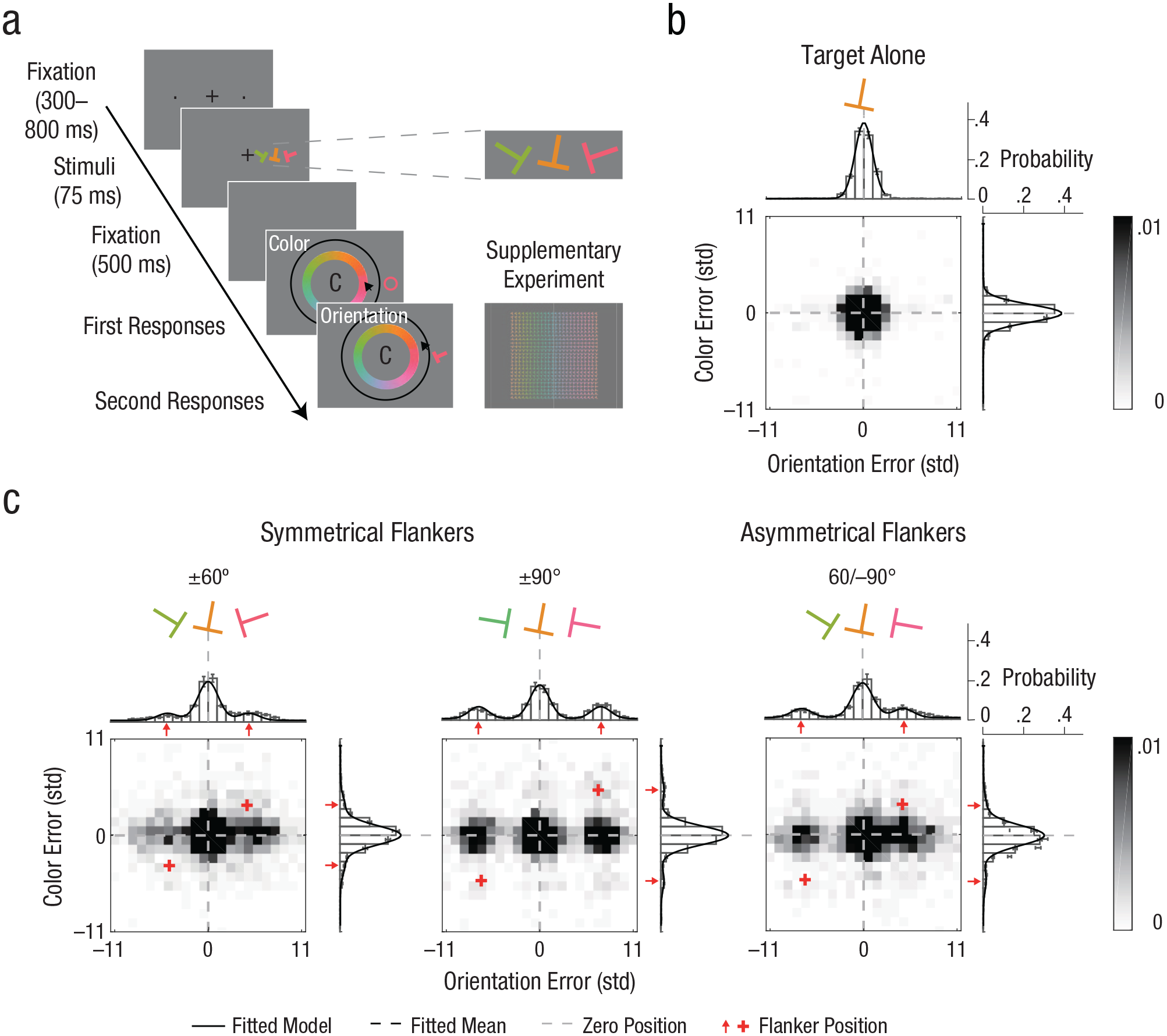
Orientation- and color-estimation tasks, stimuli, conditions, and results in Experiment 1. On each trial (a), observers viewed a T-shaped target and then had to report the target’s color and orientation. The target could appear alone (target-alone condition), flanked by two symmetrical T-shaped items (±60 and ±90 flanker conditions), or flanked by two asymmetrical T-shaped items (60/–90 flanker condition). In Experiment 1, the order of reports (orientation and color) alternated across blocks and was counterbalanced for each observer. In the Supplementary Experiment (see the Supplemental Material available online), observers reported color and orientation simultaneously. The distribution of errors relative to target feature values is shown separately for (b) the target-alone condition and (c) each of the flanker conditions. Error distributions are plotted as a function of the deviation between the estimation report and the target’s feature value for orientation (bars above heat map), color (bars to the right of heat map), and their conjunction (heat map). The axes are in units of standard deviation (std) of the error distribution in target-alone trials. Data from asymmetrical flankers were aligned to 60°/–90° (as pictured) during analysis. Solid lines indicate the response probabilities predicted by the standard model in the target-alone condition and by the standard misreport model in the flanker conditions.

Method

Observers

Fourteen undergraduate and graduate students from New York University participated in this experiment (5 female; age: range = 18–29 years, M = 21.00, SD = 3.28). On the basis of an a priori power analysis using effect sizes from previous studies (Ester et al., 2014), we estimated that a sample size of 12 observers was required to detect a crowding effect with 95% power, given a .05 significance criterion. We collected data from 2 more observers in anticipation of possible dropouts or equipment failure. All observers were naive to the purposes of the experiment. All observers were checked for normal color vision and reported having normal or corrected-to-normal visual acuity. Written informed consent was obtained from all observers before the experiment. The University Committee on Activities Involving Human Subjects at New York University approved the experimental procedures.

Apparatus

Stimuli were programmed in MATLAB (The MathWorks, Natick, MA) with the Psychophysics Toolbox extensions (Kleiner, Brainard, & Pelli, 2007) and presented on a gamma-corrected 21-in. CRT monitor (Sony GDM-5402; 1,280 × 960 resolution and 85-Hz refresh rate) connected to an iMac. A chin rest was used at a viewing distance of 57 cm. Colors and luminance were calibrated using a SpectraScan Spectroradiometer PR-670 (Photo Research, Syracuse, NY) spectrometer. Eye movements were monitored and recorded by an EyeLink 1000 (SR Research, Kanata, Ontario, Canada) infrared eye tracker. Observers used the mouse to generate responses.

Stimuli and procedure

Figure 1a illustrates a trial sequence. Each trial began with a fixation mark—a centered black plus sign subtending 0.5°—along with two dots subtending 0.05° in radius. The dots were presented on the horizontal meridian, one in the left hemifield and the other in the right hemifield. Each dot was centered at an eccentricity of 7° and indicated the two possible target locations. Following observer fixation (for a random duration between 300 and 800 ms), the stimulus display appeared for 75 ms. In the stimulus display, the target was a T-shaped item, subtending 1.6° × 1.6° and drawn with a 0.3° stroke. The target was presented on the horizontal meridian in either the left or right (randomly selected) hemifields and was centered at 7° eccentricity. The orientation and color of the target were each independently selected at random from two circular parameter spaces. Target orientation was randomly selected out of 180 values evenly distributed between 1° and 360°. Target color was randomly selected out of 180 values evenly distributed along a circle in the DKL color space (Derrington et al., 1984; see Supplementary Method 1 in the Supplemental Material). Stimuli color and background were equiluminant (56 cd/m²).

The target could be either alone (target-alone condition) or flanked by two similar T-shaped items (flanker conditions) centered on the horizontal meridian to the left and to the right of the target (each 2.1° of center-to-center distance from the target). To monitor eye fixation and stimulus eccentricity, we used on-line eye tracking (see the Apparatus section). The trials in which the observer broke fixation (> 1.5° from fixation) were terminated and rerun at the end of the block.

The stimulus display was followed by a blank interval of 500 ms, which was then followed by the response displays, which remained on screen until the observer completed both responses. The response displays included an orientation circle (a black circle 0.08° thick with an inner radius of 3.8° around the center of the screen) along with a color wheel (1.5° thick with an inner radius of 2.25°) containing the 180 colors. Observers were asked to estimate the target orientation by pointing and clicking the mouse cursor at a position on the orientation wheel and to estimate the target color by pointing and clicking the mouse cursor at a position on the color wheel. During report, a visual feedback of the selected feature was presented at the location of the target. A letter at fixation (either an O for orientation first or a C for color first) indicated report order, which was counterbalanced across blocks.

Design

Phase 1

To test the appropriateness of the estimation task with the equiluminant DKL colors, we tested the target-alone condition. Figure S1 illustrates the color-estimation values as a function of target color values for the selected eccentricity. The results showed a linear relation between estimation and target color values, ruling out the possibility that the task was mediated by color categories (e.g., red, blue).

Phase 2

There were four conditions: three flanker conditions (±60, 60/–90, and ±90; Fig. 1c) and the target-alone condition (Fig. 1b). Flankers’ orientation and color differed from those of the target by either ±60° or ±90° in orientation space and DKL color space. Each flanker had the same absolute target–flanker difference in both feature dimensions. Within each feature dimension, one flanker had a positive target–flanker difference and the other a negative target–flanker difference (randomly selected); each flanker had a unique relation to the target (negative or positive) in both feature dimensions. This design enabled us to track the direction of estimation errors related to each flanker in both feature dimensions. The three flanker conditions were based on the combinations of the target–flanker differences with the two flankers: (a) 60° and −60°, (b) 90° and −90°, and (c) 60° and −90° or 90° and −60°, which were labeled (a) ±60, (b) ±90, and (c) 60/–90, respectively. Each condition had 200 trials (800 trials overall). Each observer completed 10 blocks of 80 trials over two 50-min sessions (5 blocks per session). In each block, there were 20 trials from each of the four conditions. Response-display order was counterbalanced across blocks. The experiment began with an 80-trial practice block. Observers were encouraged to take a short rest between blocks.

Models and analyses

We analyzed the error distributions by fitting probabilistic-mixture models, which were developed from the standard model and the standard-with-misreporting model (Bays, Catalao, & Husain, 2009): For each trial, we calculated the estimation error for orientation and color by subtracting the estimation value from the true value of the target. In the flanker conditions, we aligned the data so that across feature dimensions, one flanker was consistently positive and the other was consistently negative. In the 60/–90 flanker condition, we aligned all data to be 60° and −90°. These alignments enabled us to track the effect of each individual flanker on the error distribution of each feature dimension separately and in conjunction with the other feature dimension. We compared five models.

The standard mixture model (Equation 1) uses a von Mises (circular) distribution to describe the probability density of the pooling estimation of the target’s feature and a uniform component to reflect the guessing in estimation. The model has two free parameters:

p (θ) = (1 - γ) f {(θ)}_{σ} + γ (\frac{1}{n}),

(1)

where θ is the value of the estimation error, γ is the proportion of trials in which observers are randomly guessing (guessing rate), f(θ)_σ is the von Mises distribution with a standard deviation σ (variability; the mean was set to zero), and n is the total number of possible values for the target’s feature.

The bias mixture model (Equation 2) has three free parameters. In addition to the variability and guessing rate, this model includes a free parameter for the mean (µ) of the error distribution:

p (θ) = (1 - γ) f {(θ)}_{μ, σ} + γ (\frac{1}{n}) .

(2)

The standard misreport model (Equation 3) has three free parameters. The model adds a misreporting component to the standard mixture model, which describes the probability of reporting one of the flankers to be the target:

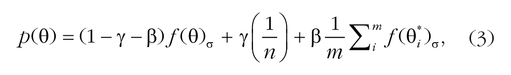
p (θ) = (1 - γ - β) f {(θ)}_{σ} + γ (\frac{1}{n}) + β \frac{1}{m} \sum_{i}^{m} f {(θ_{i}^{*})}_{σ},

(3)

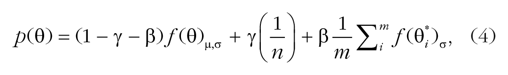
where β is the probability of reporting a flanker as the target, m is the total number of nontarget items (two in the present study), and $θ_{i}^{*}$ is the error to the feature of the ith flanker. Notice that f (θ), the von Mises distribution of the estimation errors, here describes the distribution when the observer correctly estimated the target’s feature; thus, its mean is zero. In contrast, for $f (θ_{i}^{*})$ , the distribution of estimating one flanker, the mean would be the feature distance of the corresponding flanker to that of the target. The variability of the distributions for each stimulus was assumed to be the same.

The bias misreport model (Equation 4) has four free parameters. In addition to the parameters in the standard misreport model, there is a free parameter for the mean (µ) of the distribution of estimating the target’s feature to better account for possible pooling and substitution:

p (θ) = (1 - γ - β) f {(θ)}_{μ, σ} + γ (\frac{1}{n}) + β \frac{1}{m} \sum_{i}^{m} f {(θ_{i}^{*})}_{σ},

(4)

The educated-guess model (Equation 5) has four free parameters. The model adds a misreporting component of the guessed stimuli other than the stimuli presented to the standard misreport model. This misreporting component is similar to the misreporting component of the flankers but has a different probability:

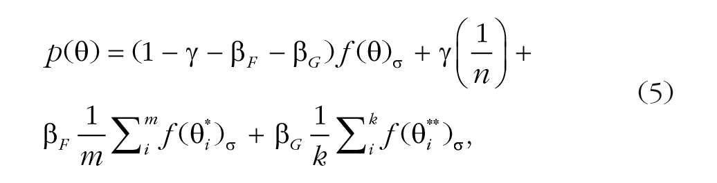
\begin{array}{l} p (θ) = (1 - γ - β_{F} - β_{G}) f {(θ)}_{σ} + γ (\frac{1}{n}) + \\ β_{F} \frac{1}{m} \sum_{i}^{m} f {(θ_{i}^{*})}_{σ} + β_{G} \frac{1}{k} \sum_{i}^{k} f {(θ_{i}^{* *})}_{σ}, \end{array}

(5)

where β_F is the probability of misreporting a flanker as the target, and β_G is the probability of misreporting a guessed feature other than the flankers presented. This model follows the assumption that the observer may have the information about one feature and then guess the feature of the target on the basis of all possible target–flanker distances. This educated guess could result in misreporting one flanker as the target or misreporting features not presented in the corresponding trial. For example, there are four possible target–flanker distances: –90°, –60°, 60°, and 90°. In a 60°/–60° trial, for each detected feature, there are five possible feature values (including the stimulus itself) that could be the possible target; therefore, there will be two flankers (–60°, 60°; m = 2) with the misreporting probability β_F, and 10 not-presented guessed stimuli (some of them are overlapped, and the nonoverlapping feature values are −150, −120, −90, −30, 30, 90, 120, and 150; k = 10) with the misreporting probability β_G.

We used the MemToolbox (Suchow, Brady, Fougnie, & Alvarez, 2013) to fit the models and compared the Akaike information criterion with correction (AICc) to assess model fits.

Results

Misreporting of orientations or colors

For each feature dimension, the estimation error was defined as the deviation between the reported and the actual feature value of the target (Figs. 1b and 1c). We analyzed the error distributions by fitting five probabilistic-mixture models to the individual data (see the Method section). All models included a von Mises (circular) distribution to describe the probability density of precision errors for the target’s feature as well as a uniform component to capture the guessing in estimation. We compared these basic-mixture models (the standard and bias models), models that also include a misreports component to describe the probability of reporting one of the flankers to be the target (the standard misreport and bias misreport models), and a model that also includes an educated-guess component to describe the proportion of observers who guessed the target on the basis of flankers’ values (the educated-guess model). We compared models by calculating AICc values for the individual model fits (Fig. 2). Table S1 in the Supplemental Material shows fitted model parameters in each condition and dimension.

Fig. 2.

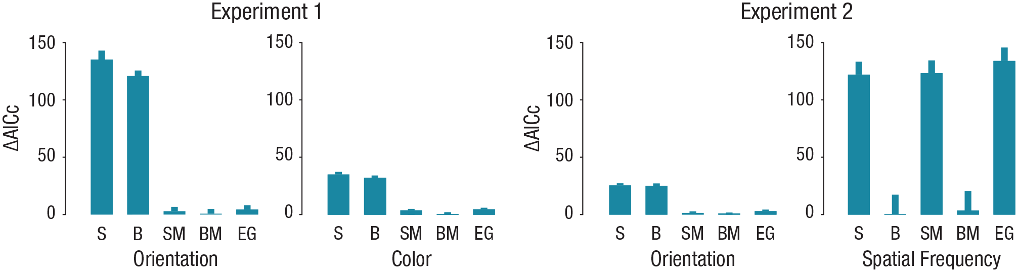
Individual goodness of fit of each of the five models to the flanker-conditions data, separately for the orientation and color reports in Experiment 1 and the orientation and spatial-frequency (SF) reports in Experiment 2. The mean Akaike information criterion with correction (AICc) was calculated by subtracting the mean AICc of the best-fitting model (lowest AICc) from the individual AICc scores of each mixture model. The five models were standard (S), bias (B), standard with misreport (SM), bias with misreport (BM), and educated guesses (EG). Error bars show +1 SEM.

To compare crowding for orientation and color, we converted each feature-dimension value with units of variability (σ) of the error distribution in target-alone trials (i.e., angle units/σ in target alone) so that in each feature dimension, target–flanker distance was presented in relation to the observer’s precision in the target-alone trials. These standardized units of target–flanker distance (±60° = ±4.60° and ±90° = ±6.90° for orientation; ±60° = ±3.43° and ±90° = ±5.15° for color) confirmed that the effect of flanker interference was comparable across feature dimensions (Figs. 1b and 1c).

On target-alone trials, the error distributions for both feature dimensions were well described by a von Mises distribution centered on the target value with an added nonzero uniform distribution (γ) for both orientation and color (Fig. 1b), t(13) = 3.03, p = .01, Cohen’s d = 0.81, and t(13) = 2.98, p = .011, Cohen’s d = 0.80, respectively, indicating that a small yet significant proportion of the responses was statistically unrelated to the target (i.e., guessing).

For both orientation and color, models with misreported components outperformed the models without the misreported component. That is, a significant proportion of errors was centered on the value of each of the two flankers, impairing the fit of a single von Mises distribution to the data. Importantly, adding an educated-guess component to the misreport model did not improve the fit, indicating that observers were unaffected by the partial correlation between target and flanker values. In the flanker conditions, the guessing rate was higher for both orientation and color, ts(13) > 2.19, ps < .05 (Tables S1 and S4 in the Supplemental Material). The misreporting rate (β) was larger than zero in all flanker conditions, ts(13) > 5.22, ps < .001. The variability (σ) of errors centered on the target increased significantly relative to the target-alone condition, ts(13) > 3.32, ps < .01, indicating that crowding led to reduced precision and increased the guessing rate and misreporting errors.

Next, we compared misreporting rates between orientation and color. Orientations were misreported more than color—orientation: averaged β = 0.27, SE = 0.03; color: averaged β = 0.086, SE = 0.01; t(13) = 7.64, p < .001, Cohen’s d = 2.04—indicating a larger crowding effect for estimation of orientation than for estimation of color.

Observers misreport orientations independently from color

To assess whether orientation and color errors occur before or after orientation and color are bound, we used trial-by-trial correlation between orientation errors and color errors to test the interdependency of crowding errors across feature dimensions. The joint distributions in each condition are presented in Figures 1b and 1c. In the target-alone condition, only 4 out of 14 observers showed a significant Pearson correlation between orientation and color errors (overall mean r = .06, SE = .04). In the flanker conditions (all three conditions collapsed), only 3 observers showed a significant correlation (overall mean r = .03, SE = .02). These findings show that orientation and color estimation were predominantly uncorrelated.

In both feature dimensions, the nature of errors was largely the same: Observers reported the orientation or color of a flanker instead of that of the target (misreporting errors). Note that it is unlikely that orientation errors were the result of combining target and flanker T-shape parts (e.g., combining target “stem” with flanker “hat”) because such combinations would lead to reporting a vast range of orientations that would be reflected by an increase in the uniform distribution rather than by misreporting errors. The misreporting errors in color could not be explained by optical blur because such blur predicts averaging errors. Importantly, orientation and color misreporting were independent from each other, suggesting that orientation and color are unbound under crowding conditions.

An alternative explanation is that the separate reports for color and orientation encouraged observers to separately encode color and orientation. Hence, the uncorrelated errors across dimensions could have been due to response strategy rather than an unbounded perceptual representation of features. To rule out this alternative explanation, we conducted a control experiment in which observers reported both orientation and color of the target with a single response. This experiment yielded converging results (see Supplementary Experiment and Fig. S2 in the Supplemental Material): Uncorrelated trial-by-trial errors were maintained even when observers simultaneously reported both dimensions. Taken together, these results show that orientation and color crowding errors occur before features are bound into an object.

Experiment 2: Orientation and SF

In this experiment, we tested whether the pattern of results obtained in Experiment 1 would also emerge with different stimuli and feature dimensions. Observers viewed sinusoidal gratings (Gabor patches) and estimated the target’s SF and orientation (Fig. 3a). These two dimensions are jointly coded by individual neurons in V1 (De Valois, Albrecht, & Thorell, 1982); thus, we hypothesized that instead of being independent, crowding errors may be interdependent.

Fig. 3.

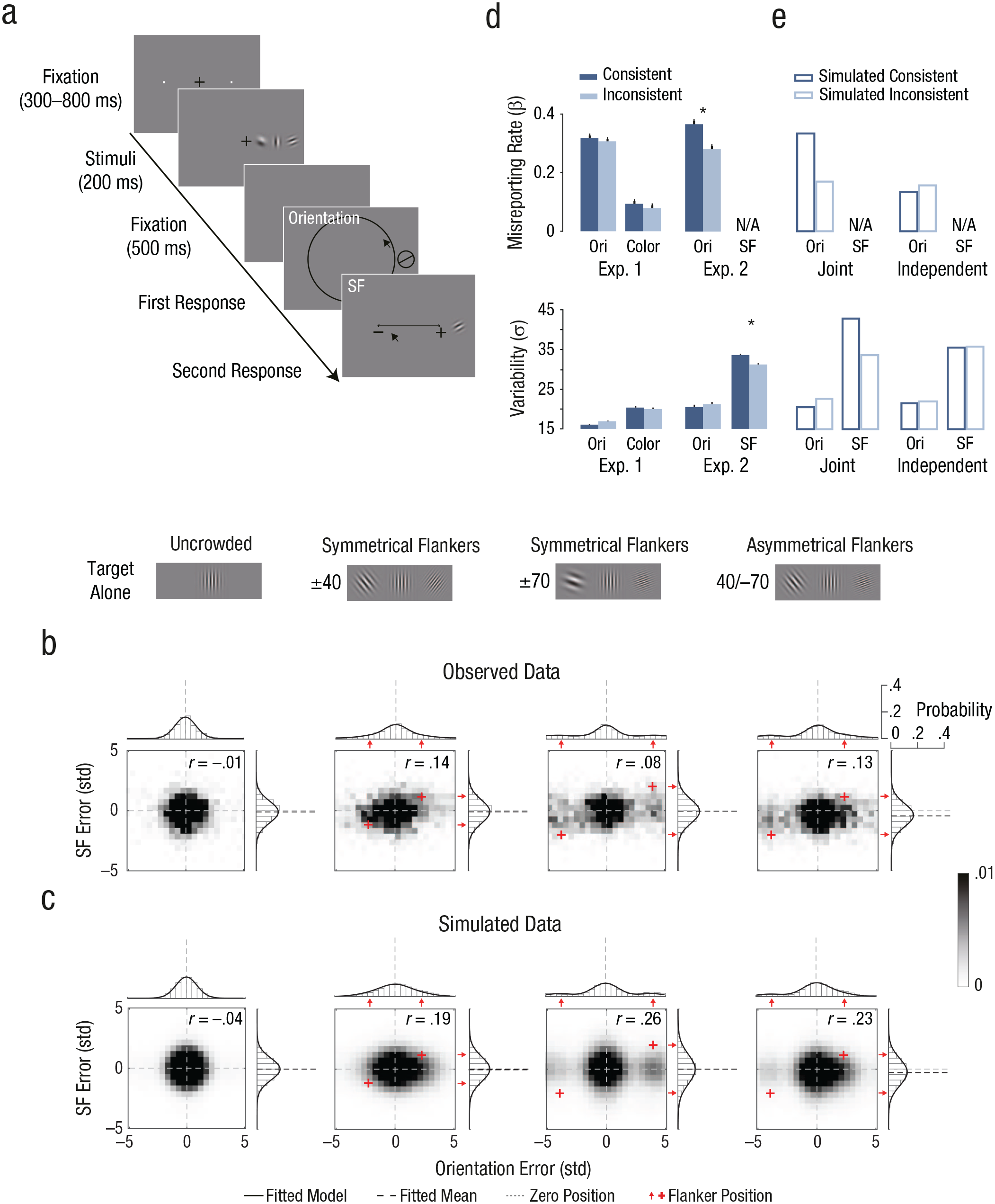
Stimuli, results, and simulated data of Experiment 2 and comparison with Experiment 1. On each trial in Experiment 2 (a), observers viewed a target Gabor patch and then had to separately report its orientation and spatial frequency. The target could appear alone (target-alone condition), flanked by two symmetrical Gabors (±40 and ±70 flanker conditions), or flanked by two asymmetrical Gabors (40/–70 flanker condition). The order of feature report (SF and orientation) alternated across blocks and was counterbalanced for each observer. The distribution of errors relative to target feature values in Experiment 2 is shown (b) for the observed data and (c) for the simulated data (by sampling 100,000 trials per condition) from the joint-coding model, separately for each condition. Error distributions are plotted as a function of the deviation between estimation report and the target’s feature value for orientation (bars above heat map), SF (bars to the right of heat map), and their conjunction (heat map). The axes are in units of standard deviation (std) of the error distribution in target-alone trials. Solid lines are model fits for orientation (standard misreport model) and SF (bias model). In (d) and (e), comparisons of misreporting rates (top panels) and standard deviations (bottom panels) in consistent and inconsistent trials are shown. Results are shown for (d) observed data in the orientation (Ori), color, and SF trials in Experiments 1 and 2 and (e) simulated data for the orientation and SF trials of the joint-coding model and independent-distribution model. Error bars show +1 SEM (Morey, 2008). Asterisks in (d) indicate significant differences between trial types (p < .01).

Method

Observers

Fourteen undergraduate students from New York University participated in this experiment (12 female; age: range = 18–21 years, M = 19.43 years, SD = 0.85). All observers were naive to the purposes of the experiment, and all reported having normal or corrected-to-normal visual acuity. Written informed consent was obtained from all observers before the experiment. The University Committee on Activities Involving Human Subjects at New York University approved the experimental procedures.

Apparatus, stimuli, procedure, and design

The se-quence of events within a trial and sample stimulus displays are presented in Figure 3a. The apparatus, stimuli, procedure, and design were the same as in Experiment 1, except for the following changes. Target and flankers were sinusoidal gratings (Gabor patches) with a 2-D Gaussian spatial envelope (SD = 0.325°, 85% contrast). The orientation and SF of the target were each randomly and independently selected from two parameter spaces. The viewing distance was 91 cm. Target and flankers’ center-to-center distance was 2.15°. The orientation parameter space ranged from 1° to 180° of visual angle. Stimulus display duration was 200 ms.

Phase 1

To determine the SF values of the estimation task, we tested the target-alone condition with different SF values, linearly spaced. On the basis of this test, we set the SF parameter space to correspond to the range of 1 to 5 cycles per degree (cpd). Because SF discriminability varies across SF values (Caelli, Brettel, Rentschler, & Hilz, 1983), we scaled the 180 unit steps of SF that were used in Phase 2 according to the variation in the estimation task of SF values in Phase 1. To do so, we fitted an exponential function to the standard deviation of the estimation data for each SF value in Phase 1 (Fig. S3 in the Supplemental Material).

Phase 2

Flankers’ orientation and SF differed from the target by either ±40 or ±70 units of orientation (°) and SF (see Phase 1). Each flanker had the same absolute target–flanker difference in both feature dimensions. Within each feature dimension, one flanker had a positive target–flanker difference and the other a negative target–flanker difference (randomly selected); each flanker had a unique relation to the target (negative or positive) in both feature dimensions. Target–flanker distance within the parameter space was (a) 40°/–40°, (b) 70°/–70°, and (c) 40°/–70° or 70°/–40°, which were labeled (a) ±40, (b) ±70, and (c) 40/–70, respectively.

In all trials, the target orientation was randomly selected from the range of 1° to 180° with a step size of 2°. In target-alone trials, the target SF was randomly selected out of the 180 steps, as determined in Phase 1. However, because SF is not a circular space, in the crowding display, flankers’ SF values restricted the range of target SF values; the target SF ranged from 41 to 140 SF steps (1.82–4.07 cpd) in the ±40 flanker condition, 71 to 110 SF steps (2.49–3.39 cpd) in the ±70 flanker condition, and 41 to 110 SF steps (1.82–3.39 cpd) and 71 to 140 SF steps (2.49–4.07 cpd) in the 40/–70 flanker condition.

There were two response displays. In the orientation response display, observers had to estimate the target orientation by pointing and clicking the mouse cursor at a position on the orientation wheel. In the SF response display, observers estimated SF by pointing and clicking the mouse cursor on a centered horizontal line (0.08°-thick two-directional arrow 11.2° in length). A minus sign on one side and a plus sign on the other indicated the direction of SF increase. Because SF is not circular, we extended the range of the SF response (0.48–7.35 cpd) beyond that of the target (1–5 cpd).

Models and analyses

Because SF is not circular, we used a Gaussian distribution when fitting SF to the mixture models and von Mises distribution when fitting orientation to the mixture models. Because we had to restrict the range of the target SF in the flanker conditions, we equated the range of target SF when comparing the SF flanker and target-alone conditions.

Results

Misreporting of orientations but averaging of SFs

Error distributions differed between orientation and SF. Whereas orientation errors were best described by misreporting models, SF errors were best described by a single Gaussian function with an added uniform distribution (bias models; Fig. 2). In both feature dimensions, the best-fitting models outperformed the educated-guess model. Table S1 shows parameters of the best-fitting model for each condition and dimension.

Orientation

As in Experiment 1, significant proportions of orientation error in the flanker conditions were due to misreporting, ts(13) > 3.6, ps < .004, and guessing, ts(13) > 3.6, ps < .003 (Fig. 3b; Table S4 includes all statistical values). But the variability of the von Mises distribution between flanker and target-alone conditions was equivalent, ts < 2.1, ps > .06. These results indicate that orientation-estimation errors were due to increases in the guessing and misreporting rates.

Spatial frequency

The variance of SF errors was larger in the flanker conditions than in the target-alone condition (Tables S1 and S4), ts(13) > 3.9, ps < .002. The proportion of guesses did not increase compared with the target-alone condition, ts(13) < 2.1, ps > .05. When we tested the mean (µ) of the Gaussian distribution (i.e., the bias of the target distribution toward a particular flanker), no effects of bias were found in ±40 and ±70 conditions compared with the target-alone condition, ts(13) < 0.8, ps > .40. Interestingly, the mean in the 40/–70 condition was significantly biased toward the −70° flanker (negative bias) compared with the target-alone condition within the same target SF range, t(13) = −4.69, p = .0004, Cohen’s d = −1.25 (Table S1). This effect on bias is consistent with averaging of the target and flanker values and inconsistent with misreporting errors because misreporting errors with the 40° flanker would have shifted the mean of the target distribution toward the 40° flanker rather than the –70° flanker.

Could the effectively smaller target–flanker distance in SF space than in orientation space, due to the larger variability in SF, lead to the SF advantage of the bias model over the bias-misreport model? Were this the case, misreporting errors in SF would emerge as the target–flanker distance increased or, conversely, when the variability in SF was reduced to that in orientation. To test this alternative explanation, we assessed misreporting rates in SF using the bias-misreport model. Figure S4a in the Supplemental Material plots misreporting rates for SF and orientation separately for the ±40 and ±70 flanker conditions as a function of target–flanker distance normalized by the baseline variability, that is, the distance in feature space divided by the variability in target-alone trials. In contrast to this prediction, results showed that SF misreporting rates were not significantly above zero when the distance was large, that is, in the ±70 flanker condition, t(13) = 1.9, p = .079. In fact, misreporting rates were larger than zero in SF space only when flanker value overlapped with target distribution, such as in the ±40 flanker conditions, t(13) = 4.3, p = .0008, Cohen’s d = 1.15. As mentioned above, misreporting rates for orientation were significantly above zero in all flanker conditions. Importantly, when comparing model fit separately for each flanker condition, we found that misreport models (mean AICc = 1,933) outperformed the standard model without misreport (mean AICc = 1,956) for orientation, whereas for SF, the bias model (mean AICc = 1,940) outperformed the bias model with misreport (mean AICc = 1,955), even when the target–flanker distance was effectively larger in SF (±70°) than in orientation (±40°; Fig. S5 in the Supplemental Material).

Furthermore, we tested whether the misreporting rate would emerge in SF when the variability is the same as in the orientation report. We compared misreporting rates between observers with baseline (target-alone) variability below the median in SF and observers with baseline variability above the median in orientation (Fig. S4b). Even when variability was similar between SF and orientation, the misreporting rate was significantly above zero for orientation, t(6) = 2.54, p = .044, Cohen’s d = 0.96, but not for SF, t(6) = 1.5, p = .18. These results show that, contrary to this alternative explanation, the misreporting rate in SF did not emerge when flanker distance was sufficiently large. Thus, assessing the bias of the mean of SF in 40/–70, assessing misreporting rates in SF using the bias-misreport model, and equating for variability in SF and orientation rule out the alternative interpretation that SF findings are due to a smaller target–flanker distance.

Observers misreport orientations interdependently of averaging of SFs

Heat maps of the joint distributions in each condition are presented in Figure 3b. Orientation and SF estimation errors were uncorrelated in the target-alone condition, and only 1 observer showed a significant linear correlation (mean r = .002, SE = .02). However, across flanker conditions, there was a significant linear correlation between orientation and SF errors (r = .138, SE = .03, ps < .0001), indicating that orientation and SF crowding errors were interdependent. Individual trial-by-trial linear correlations showed a significant (ps < .04) correlation in 10 out of 14 observers (mean r = .14, SE = .03).

To further assess the interdependency of crowding errors across feature dimensions and to compare the interdependency in Experiments 1 and 2, we analyzed the distribution of errors in one dimension on the basis of observers’ errors in the other dimension. That is, we tested whether the direction (with respect to flanker values) of an error in one feature dimension was dependent on the direction of the error in the other feature dimension (see the Method section). To do so, we divided trials into two groups: trials in which estimation errors for both features (orientation vs. color or SF) were toward the same flanker (consistent trials) and trials in which errors for each feature were toward separate flankers (inconsistent trials). In Figure 3d, we plot the effects of consistent versus inconsistent errors across dimension on misreporting rates and estimation variability for color (Experiment 1), orientation (Experiments 1 and 2), and SF (Experiment 2). The effect of consistency was found between orientation-misreporting rate, F(1, 13) = 11.2, p = .005, η_g² = .05, and SF variability, F(1, 13) = 19.86, p = .0006, η_g² = .02, but not between orientation and color (all ps > .10; for detailed results, see Supplementary Results, Table S4, and Fig. S6 in the Supplemental Material).

Simulation of pooling of a joint population coding can explain orientation and SF crowding

To test whether the results of Experiment 2 could be explained by a representation in which orientations and SFs were bound, we compared the fit of two versions of a biologically plausible computational model that simulates a population of neurons. In the joint-coding-model version, the populations jointly code orientations and SFs (Fig. 4; see also Supplementary Method 2 and Table S2 in the Supplemental Material), whereas in the independent-coding-model version, the populations separately code orientations and SFs (Table S in the Supplemental Material). The models rely on population-coding principles and explain crowding as a weighted sum of target and flanker feature values within a receptive field (Harrison & Bex, 2015; van den Berg et al., 2010). We used a single bivariate Gaussian distribution to simulate the joint coding of orientation and SF and two univariate normal distributions to simulate the separate representation of orientation and color. The model assumes pooling over a larger region of space for SF than orientation to explain averaging in SF reports and misreporting in orientation reports. This assumption is related to the fact that SF judgments involve assessing the width and distance of multiple cycles inside the Gabor patch (Robson & Graham, 1981), whereas the orientation judgment may involve assessing a more narrow region of space, for example, a region with a higher aspect ratio (Goris, Simoncelli, & Movshon, 2015). In the simulation, coding precisions (the inverse of the standard deviation of the Gaussian response function) and the standard deviation of the Gaussian receptive field were directly responsible for orientation-estimation variability and misreporting rate, respectively. Therefore, these parameters were determined on the basis of the fitting of the probabilistic standard misreport model to the observed orientation data. Both simulated models were fitted to the results of Experiment 2 (both r²s = .88). However, unlike in Experiment 2, the independent-coding model showed no correlation between orientation and SF (mean r = 0) and no effect of consistency (Fig. 3e). The joint-coding model, on the other hand, showed the same interdependent pattern as the results of Experiment 2 (Fig. 3c), including the correlation between orientation and SF (mean r = .23) and the increase in the misreporting rate of orientations and standard deviation of SF in consistent versus inconsistent trials (Fig. 3e). These results support the conclusion that joint coding of orientation and SF underlies the results of Experiment 2.

Fig. 4.

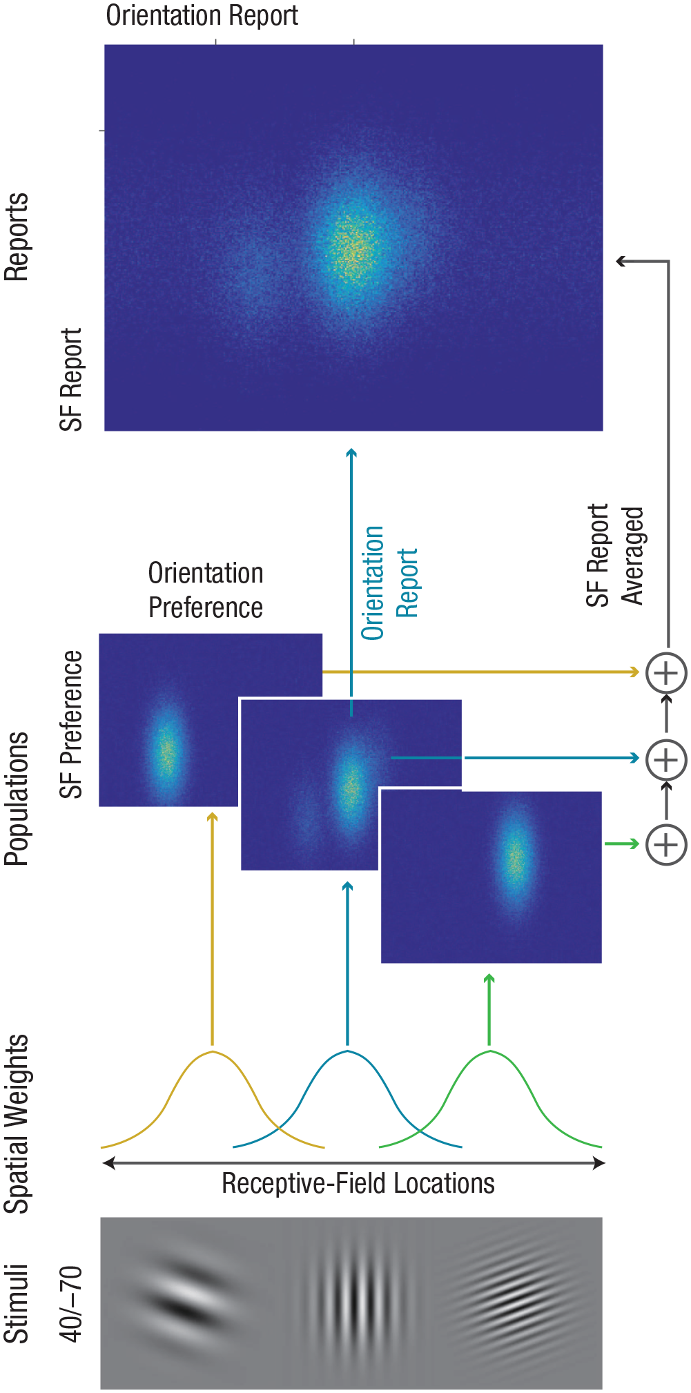
Simulation of population neural activity that jointly codes for orientation and spatial frequency (SF) fitted to Experiment 2. The model simulates the firing rates of three populations of neurons with receptive-field locations, orientation preference, and SF preference. Stimuli consisted of a target presented with two flankers (asymmetrical flanker condition: 40/–70). A normalized Gaussian function determined the population level to a stimulus as a function of its relative distance (compared with other stimuli) from the center of receptive field (spatial weights). Population neural activity in response to each location was described by a bivariate probability function with orientation preference (horizontal) and SF preference (vertical). Orientation and SF arrangement is centered over the target-orientation and SF values. Report of orientation is based on a single population over the target location. Report of SF is based on pooling over different locations, that is, pooling with receptive field centered over each location.

Discussion

In this study, we simultaneously characterized the pattern of crowding errors within and between feature dimensions. In three experiments, we demonstrated variations in the pattern of crowding errors based on the specific feature dimensions (orientation, color, and SF) and their conjunctions. Crowding is more pronounced for orientation than for color. Crowding reflects misreporting a flanker orientation or color instead of those of the target but averaging of their SFs. The pattern of results was contingent on the feature-dimension type but not the stimulus type: Observers misreported the target orientation regardless of whether the stimulus was a colored T or a grating. The distinct pattern of crowding errors in each dimension suggests a distinct representation for each feature dimension.

Crowding errors for orientation and SF were interdependent, but those for orientation and color were independent. These findings were shown by the analysis of the joint distribution of feature-dimension errors and trial-by-trial correlations. Moreover, comparison of model parameters revealed higher orientation misreporting rates when SF and orientation errors were toward the same flanker, but that was not the case for orientation and color. These findings suggest that the spatial integration that underlies crowding operates after orientation is bound with SF but before it is bound with color.

Not all features behave the same under crowding: errors within feature dimensions

The present study challenges many models’ implicit assumption that crowding operates in the same manner across different feature dimensions (Pelli & Tillman, 2008; Whitney & Levi, 2011). Investigations supporting this view had not tested for qualitative differences in the pattern of errors across dimensions (Greenwood et al., 2012; Põder & Wagemans, 2007; van den Berg et al., 2007). Here, within the same display, we showed both quantitative and qualitative differences in the pattern of errors across different dimensions. First, orientation misreporting was 3 times more likely than color misreporting, demonstrating that estimation of orientation is more susceptible to crowding than estimation of color. Second, whereas orientation or color was misreported, SFs were averaged in the SF dimension. This variation between misreporting and averaging occurred within the same stimuli and display (Gabor patch). It has been proposed that observed errors may be contingent on the target–flankers orientation distance (Harrison & Bex, 2015; Mareschal, Morgan, & Solomon, 2010; but see Ester et al., 2015). Here, variation between misreporting errors and averaging errors cannot be explained by target–flanker distance. Observers misreported orientation and averaged SF even when the distance in feature space was effectively the same (Figs. S4b and S5). Thus, this study shows that crowding varies as a function of the feature dimension being reported.

Crowding and feature binding: errors between feature dimensions

Numerous studies have demonstrated observers’ failure to correctly report the conjunction of feature dimensions of peripheral items (e.g., color and shape), that is, misbinding errors, also known as illusory conjunctions (e.g., Dowd & Golomb, 2019; Vul & Rich, 2010; for a review, see Di Lollo, 2012). According to popular views, outside the focus of attention, independent sampling of individual features occurs under location uncertainties and therefore leads to the misbinding of features (Treisman & Schmidt, 1982; Vul & Rich, 2010). Although investigations of misbinding errors have often manipulated attention (Dowd & Golomb, 2019; Vul & Rich, 2010), many of these studies were conducted using a crowded display, that is, stimuli spacing was below the critical space of crowding (Pelli et al., 2004), suggesting that at least some misbinding errors can be explained with the same processes underlying crowding. However, whereas crowding errors are characterized by errors within a particular feature dimension (that can lead to either averaging or misreporting), investigations of misbinding errors in the visual periphery have focused on errors between feature dimensions. For example, Vul and Rich (2010) investigated misbinding errors by manipulating top-down attention and analyzing error distributions in the location space of categorical forced-choice reports for color and shape (letter); therefore, they assessed only errors between feature dimensions. Yet, until now, no study had directly investigated the relations between crowding errors (or errors within feature dimensions) and misbinding errors (or errors between feature dimensions).

In this study, by using dual continuous-estimation reports of two simultaneously presented feature dimensions, we were able to quantitatively assess errors due to crowding both within and between feature dimensions. The results reveal that in a crowded display, color and orientation remain unbound, even when both dimensions are jointly reported. Unlike color, SF remains bound with orientation in crowding displays; observers tended to misreport flanker orientation and average SF with the same flanker. This contingency of binding errors on the specific feature dimensions may explain why some studies using a set of stimuli suggested that crowding reflects interference in feature binding (Pelli et al., 2004; Põder & Wagemans, 2007), whereas another study using a different set of stimuli suggested that crowding follows feature binding (Greenwood et al., 2012).

Conclusion

This study directly links two mostly independent topics of research—crowding and feature binding—and challenges conventional views in each of them. By testing crowding both within and between feature dimensions, we showed that it is not a uniform phenomenon: It reflects different operations depending on the specific feature dimensions and their conjunctions. Both the data analysis and our model simulation suggest that crowding reflects spatial integration over neural populations that encode both orientation and SF together but color separately.

Supplemental Material

Yashar_OpenPracticesDisclosure_rev – Supplemental material for Crowding and Binding: Not All Feature Dimensions Behave in the Same Way

Supplemental material, Yashar_OpenPracticesDisclosure_rev for Crowding and Binding: Not All Feature Dimensions Behave in the Same Way by Amit Yashar, Xiuyun Wu, Jiageng Chen and Marisa Carrasco in Psychological Science

Supplemental Material

Yashar_Supplemental_Material_rev – Supplemental material for Crowding and Binding: Not All Feature Dimensions Behave in the Same Way

Supplemental material, Yashar_Supplemental_Material_rev for Crowding and Binding: Not All Feature Dimensions Behave in the Same Way by Amit Yashar, Xiuyun Wu, Jiageng Chen and Marisa Carrasco in Psychological Science

Footnotes

Acknowledgements

We thank Denis Pelli and members of the Carrasco Lab for their useful comments.

Action Editor

Edward S. Awh served as action editor for this article.

Author Contributions

A. Yashar and M. Carrasco developed the study concept. All the authors contributed to the study design. A. Yashar, X. Wu, and J. Chen collected pilot data. X. Wu collected experimental data. A. Yashar and X. Wu analyzed the data. A. Yashar, X. Wu, and M. Carrasco interpreted the data. A. Yashar and X. Wu drafted the manuscript, and M. Carrasco provided critical revisions and edited the manuscript. All the authors approved the final manuscript for submission.

ORCID iD

Amit Yashar

Declaration of Conflicting Interests

The author(s) declared that there were no conflicts of interest with respect to the authorship or the publication of this article.

Funding

This work was supported by Israel Science Foundation Grant Nos. 1980/18 and 111/15 (to A. Yashar) and National Institutes of Health Grant No. R01-EY016200 (to M. Carrasco).

Supplemental Material

Additional supporting information can be found at

Open Practices

All data and materials have been made publicly available via the Open Science Framework and can be accessed at osf.io/vy62h. The design and analysis plans for this study were not preregistered. The complete Open Practices Disclosure for this article can be found at http://journals.sagepub.com/doi/suppl/10.1177/0956797619870779. This article has received the badges for Open Data and Open Materials. More information about the Open Practices badges can be found at .

References

Bays

P. M.

Catalao

R. F. G.

Husain

(2009). The precision of visual working memory is set by allocation of a shared resource. Journal of Vision, 9(10), Article 7. doi:10.1167/9.10.7

Bouma

(1970). Interaction effects in parafoveal letter recognition. Nature, 226, 177–178. doi:10.1038/226177a0

Caelli

Brettel

Rentschler

Hilz

(1983). Discrimination thresholds in the two-dimensional spatial frequency domain. Vision Research, 23, 129–133.

Derrington

A. M.

Krauskopf

Lennie

(1984). Chromatic mechanisms in lateral geniculate nucleus of macaque. The Journal of Physiology, 357, 241–265.

De Valois

R. L.

Albrecht

D. G.

Thorell

L. G

. (1982). Spatial frequency selectivity of cells in macaque visual cortex. Vision Research, 22, 545–559. doi:10.1016/0042-6989(82)90113-4

Di Lollo

. (2012). The feature-binding problem is an ill-posed problem. Trends in Cognitive Sciences, 16, 317–321. doi:10.1016/j.tics.2012.04.007

Dowd

E. W.

Golomb

J. D.

(2019). Object-feature binding survives dynamic shifts of spatial attention. Psychological Science, 30, 343–361. doi:10.1177/0956797618818481

Ester

E. F.

Klee

Awh

(2014). Visual crowding cannot be wholly explained by feature pooling. Journal of Experimental Psychology: Human Perception and Performance, 40, 1022–1033. doi:10.1037/a0035377

Ester

E. F.

Zilber

Serences

J. T.

(2015). Substitution and pooling in visual crowding induced by similar and dissimilar distractors. Journal of Vision, 15(1), Article 4. doi:10.1167/15.1.4

10.

Freeman

Simoncelli

E. P.

(2011). Metamers of the ventral stream. Nature Neuroscience, 14, 1195–1201. doi:10.1038/nn.2889

11.

Goris

R. L. T.

Simoncelli

E. P.

Movshon

J. A.

(2015). Origin and function of tuning diversity in macaque visual cortex. Neuron, 88, 819–831. doi:10.1016/j.neuron.2015.10.009

12.

Greenwood

J. A.

Bex

P. J.

Dakin

S. C.

(2009). Positional averaging explains crowding with letter-like stimuli. Proceedings of the National Academy of Sciences, USA, 106, 13130–13135. doi:10.1073/pnas.0901352106

13.

Greenwood

J. A.

Bex

P. J.

Dakin

S. C.

(2010). Crowding changes appearance. Current Biology, 20, 496–501. doi:10.1016/j.cub.2010.01.023

14.

Greenwood

J. A.

Bex

P. J.

Dakin

S. C.

(2012). Crowding follows the binding of relative position and orientation. Journal of Vision, 12(3), Article 18. doi:10.1167/12.3.18

15.

Harrison

W. J.

Bex

P. J.

(2015). A unifying model of orientation crowding in peripheral vision. Current Biology, 25, 3213–3219. doi:10.1016/j.cub.2015.10.052

16.

Huckauf

Heller

(2014). What various kinds of errors tell us about lateral masking effects. Visual Cognition, 9, 889–910. doi:10.1080/13506280143000548A

17.

Keshvari

Rosenholtz

(2016). Pooling of continuous features provides a unifying account of crowding. Journal of Vision, 16(3), Article 39. doi:10.1167/16.3.39

18.

Kimchi

Pirkner

(2015). Multiple level crowding: Crowding at the object parts level and at the object configural level. Perception, 44, 1275–1292.

19.

Kleiner

Brainard

D. H.

Pelli

D. G.

(2007). What’s new in Psychtoolbox-3? Perception, 36(ECVP Abstract Suppl.).

20.

Levi

D. M.

(2008). Crowding—An essential bottleneck for object recognition: A mini-review. Vision Research, 48, 635–654. doi:10.1016/j.visres.2007.12.009

21.

Levi

D. M.

Klein

S. A.

(1986). Sampling in spatial vision. Nature, 320, 360–362. doi:10.1038/320360a0

22.

Manassi

Whitney

(2018). Multi-level crowding and the paradox of object recognition in clutter. Current Biology, 28, R127–R133. doi:10.1016/j.cub.2017.12.051

23.

Mareschal

Morgan

M. J.

Solomon

J. A.

(2010). Cortical distance determines whether flankers cause crowding or the tilt illusion. Journal of Vision, 10(8), Article 13. doi:10.1167/10.8.13

24.

Morey

R. D.

(2008). Confidence intervals from normalized data: A correction to Cousineau (2005). Tutorials in Quantitative Methods for Psychology, 4, 61–64. doi:10.3758/s13414-012-0291-2

25.

Nandy

A. S.

Tjan

B. S.

(2012). Saccade-confounded image statistics explain visual crowding. Nature Neuroscience, 15, 463–469. doi:10.1038/nn.3021

26.

Parkes

Lund

Angelucci

Solomon

J. A.

Morgan

(2001). Compulsory averaging of crowded orientation signals in human vision. Nature Neuroscience, 4, 739–744.

27.

Pelli

D. G.

Palomares

Majaj

N. J.

(2004). Crowding is unlike ordinary masking: Distinguishing feature integration from detection. Journal of Vision, 4, 1136–1169. doi:10.1167/4.12.12

28.

Pelli

D. G.

Tillman

K. A.

(2008). The uncrowded window of object recognition. Nature Neuroscience, 11, 1129–1135.

29.

Põder

Wagemans

(2007). Crowding with conjunctions of simple features. Journal of Vision, 7(2), Article 23. doi:10.1167/7.2.23

30.

Robson

J. G.

Graham

(1981). Probability summation and regional variation in contrast sensitivity across the visual field. Vision Research, 21, 409–418.

31.

Scolari

Kohnen

Barton

Awh

(2007). Spatial attention, preview, and popout: Which factors influence critical spacing in crowded displays? Journal of Vision, 7(2), Article 7. doi:10.1167/7.2.7

32.

Strasburger

Harvey

L. O.

Rentschler

(1991). Contrast thresholds for identification of numeric characters in direct and eccentric view. Perception & Psychophysics, 49, 495–508. doi:10.3758/BF03212183

33.

Suchow

J. W.

Brady

T. F.

Fougnie

Alvarez

G. A.

(2013). Modeling visual working memory with the MemToolbox. Journal of Vision, 13(10), Article 9. doi:10.1167/13.10.9

34.

Treisman

Schmidt

(1982). Illusory conjunctions in the perception of objects. Cognitive Psychology, 14, 107–141. doi:10.1016/0010-0285(82)90006-8

35.

van den Berg

Roerdink

J. B. T. M.

Cornelissen

F. W

. (2007). On the generality of crowding: Visual crowding in size, saturation, and hue compared to orientation. Journal of Vision, 7(2), Article 14. doi:10.1167/7.2.14

36.

van den Berg

Roerdink

J. B. T. M.

Cornelissen

F. W

. (2010). A neurophysiologically plausible population code model for feature integration explains visual crowding. PLOS Computational Biology, 6(1), Article e1000646. doi:10.1371/journal.pcbi.1000646

37.

Vul

Rich

A. N.

(2010). Independent sampling of features enables conscious perception of bound objects. Psychological Science, 21, 1168–1175. doi:10.1177/0956797610377341

38.

Whitney

Levi

D. M.

(2011). Visual crowding: A fundamental limit on conscious perception and object recognition. Trends in Cognitive Sciences, 15, 160–168. doi:10.1016/j.tics.2011.02.005

39.

Yashar

Chen

Carrasco

(2015). Rapid and long-lasting reduction of crowding through training. Journal of Vision, 15(10), Article 15. doi:10.1167/15.10.15

Supplementary Material

Please find the following supplemental material available below.

For Open Access articles published under a Creative Commons License, all supplemental material carries the same license as the article it is associated with.

For non-Open Access articles published, all supplemental material carries a non-exclusive license, and permission requests for re-use of supplemental material or any part of supplemental material shall be sent directly to the copyright owner as specified in the copyright notice associated with the article.

0.00 MB

0.28 MB

1.71 MB